The baryon budget on the galaxy group/cluster boundary

Abstract

We present a study of the hot gas and stellar content of 5 optically-selected poor galaxy clusters, including a full accounting of the contribution from intracluster light (ICL) and a combined hot gas and hydrostatic X-ray mass analysis with XMM-Newton observations. We find weighted mean stellar (including ICL), gas and total baryon mass fractions within $r_{\mathrm{500}}$ of $0.026\pm 0.003$, $0.070\pm 0.005$ and $0.096\pm 0.006$ , respectively, at a corresponding weighted mean $M_{\mathrm{500}}$ of ($1.08_{-0.18}^{+0.21})\times 10^{14}$ M_⊙. Even when accounting for the intracluster stars, 4 out of 5 clusters show evidence for a substantial baryon deficit within $r_{\mathrm{500}}$, with baryon fractions ($f_{\mathrm{b}}$) between 50$\pm$6 to 59$\pm$8 per cent of the Universal mean level (i.e. $\Omega_{b}/\Omega_{m}$); the remaining cluster having $f_{\mathrm{b}}$ = 75$\pm$11 per cent. For the 3 clusters where we can trace the hot halo to $r_{\mathrm{500}}$ we find no evidence for a steepening of the gas density profile in the outskirts with respect to a power law, as seen in more massive clusters. We find that in all cases, the X-ray mass measurements are larger than those originally published on the basis of the galaxy velocity dispersion ($\sigma$) and an assumed $\sigma-M_{\mathrm{500}}$ relation, by a factor of 1.7–5.7. Despite these increased masses, the stellar fractions (in the range 0.016–0.034, within $r_{\mathrm{500}}$) remain consistent with the trend with mass published by Gonzalez et al. (2007), from which our sample is drawn.

1 Introduction

The hot gas and stellar content of collapsed structures are key elements in the baryon budget of the Universe. Conducting a full census of these baryons is particularly important given the likely effects of non-gravitational heating and radiative cooling (e.g. Voit & Bryan, 2001) on the hot gas and star formation. Both these mechanisms raise the entropy of the intracluster medium (ICM), either by heating it directly or else condensing out the lowest entropy gas from the hot phase, but each produces a different balance of hot and cold baryons. However, tracking all of the baryons is observationally challenging, particularly in the lowest mass haloes, where feedback may be more influential. In such cases, hot gas may have been displaced to the group/cluster outskirts or even ejected from the (progenitor) halo altogether (e.g. McCarthy et al., 2011). Moreover, a substantial fraction of the cold baryons may be locked up in intracluster stars, whose diffuse and low surface brightness emission is very difficult to detect (e.g. Feldmeier et al., 2002; Zibetti et al., 2005; Gonzalez et al., 2005; Krick & Bernstein, 2007).

Cluster name	RAa	Dec.a	Redshift	Hi Columnb	Obsidc	Observation Date	$t_{\mathrm{MOS1}}$	$t_{\mathrm{MOS2}}$	$t_{\mathrm{pn}}$
	(J2000)	(J2000)		($\times 10^{20}$ cm-2)			(ks)	(ks)	(ks)
Abell 2401	21 58 22.5	-20 06 15	0.0571	2.39	0555220101	2010 Oct 29	54.6	54.7	41.8
Abell 2955	01 56 59.8	-17 02 23	0.0943	1.77	0555220201	2008 Aug 02	75.6	75.5	51.5
Abell S0296	02 46 51.5	-42 22 41	0.0696	1.86	0555220301	2008 Dec 26	50.7	52.9	34.1

Table 1: Key properties of the 3 galaxy clusters with new XMM-Newton data. ^aCoordinates of the brightest cluster galaxy, on which the X-ray halo is centred. ^bGalactic Hi column, interpolated to the cluster centroid using the data of Kalberla et al. (2005). ^cXMM-Newton observation identifier. The last 3 columns are the effective exposure times for the MOS and pn detectors after flare filtering.

The importance of the ICL in the baryon budget is the subject of current debate, with different methods giving a range of estimates for its contribution to the total cluster stellar light. For example, direct measurements by Krick & Bernstein (2007) suggest an ICL fraction of 6–22 per cent in the $r$ band, within 25 per cent of the virial radius, while Gonzalez et al. (2005, 2007) estimate that the combined contribution of the brightest cluster galaxy and ICL amounts on average to 33 per cent of the total stellar light within $r_{\mathrm{200}}$, based on detailed $I$ band imaging of 24 clusters. In contrast, McGee & Balogh (2010) find a $\sim$50 per cent contribution, based on mapping of hostless type Ia supernovae. In one of the largest studies of its kind, Zibetti et al. (2005) favour a lower contribution, of $\sim$11 per cent within 500 kpc, based on stacking Sloan Digital Sky Survey (SDSS) images of 683 clusters. However, the use of stacking to map the ICL will tend to bias the inferred measurements towards lower values, if uncollapsed systems are included in the sample. The relatively wide variation in ICL estimates may partly be due to differences in sample selection. For example, the Gonzalez et al. study preferrentially includes systems with a prominent brightest cluster galaxy (BCG).

On the other hand, the contribution of hot gas is better determined, and represents the largest component of the baryon budget in clusters. However, the best constraints are based on X-ray selected (and often archival) samples (e.g. Vikhlinin et al., 2006; Arnaud et al., 2007; Sun et al., 2009), which are biased towards haloes with more centrally concentrated hot gas (e.g. Rykoff et al., 2008b; Dai et al., 2010; Balogh et al., 2011). Furthermore, there is a long-standing tendency for X-ray studies to target different clusters to those best studied at optical/(near)-infrared wavelengths. A full accounting of hot gas and stars (including ICL) in the same systems is therefore lacking, but is clearly essential to establish the overall balance and uncover any missing baryons. This is best achieved by securing X-ray observations of optically well-studied clusters, given the difficulty of mapping the ICL directly.

The goal of this paper is, for the first time, to combine X-ray observations of the hot gas in low-mass clusters with a full galaxy + ICL stellar mass analysis, using the former to measure both the gas and total mass. This approach calls for X-ray follow-up observations of clusters for which the ICL analysis has already been completed, given the difficulty of directly mapping diffuse optical light. The low-mass scale is particularly interesting to study since it encompasses the regime where cluster properties become increasingly diverse and where there is a more equal balance between hot and cold baryons (e.g. Gonzalez et al., 2007). Our clusters were drawn from the optically-selected sample of Gonzalez et al. (2007, hereafter GZZ07), with the aim of targeting the lowest mass objects ($\sigma\la 500\mbox{~{}km}\mbox{~{}s}^{-1}$) with the best quality optical data, for which the gas and total mass within $r_{\mathrm{500}}$ could be measured by XMM-Newton in a reasonable exposure time ($r_{\mathrm{500}}$ being the radius enclosing an overdensity of 500 with respect to the critical density).

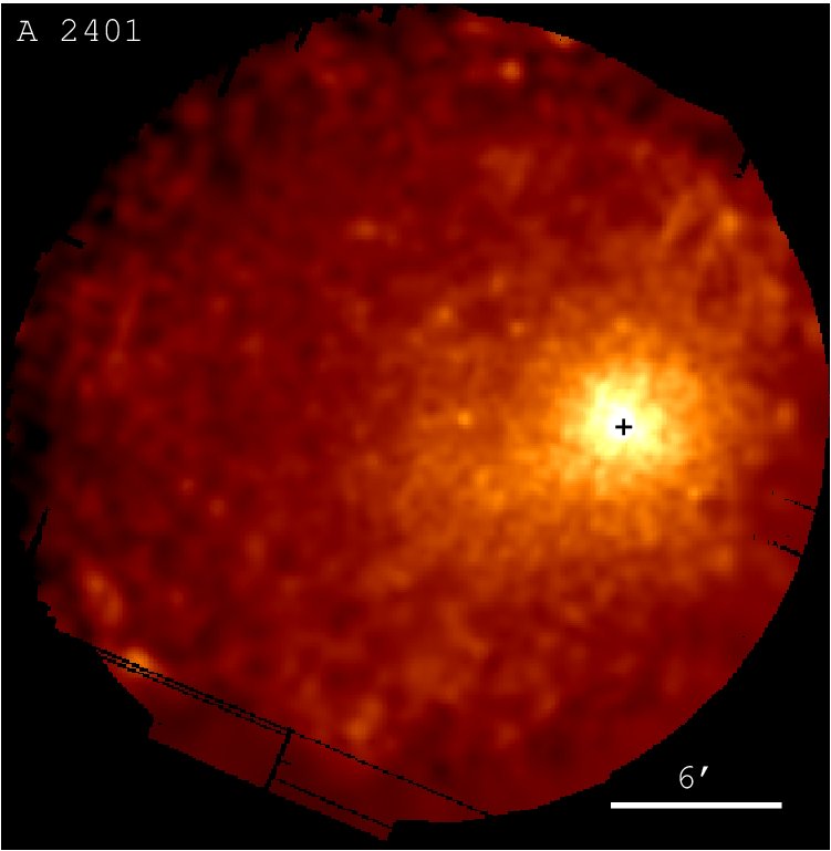
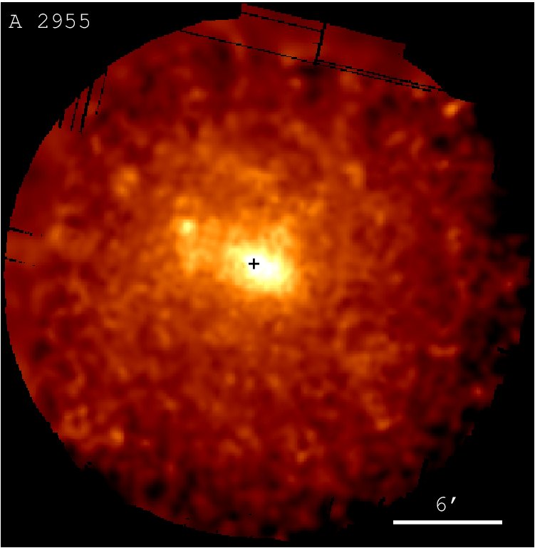
Figure 1: Combined 0.3–2.0 keV MOS/pn XMM-Newton images of the diffuse emission from the 3 newly observed clusters, with point-like sources removed and filled using the ciao task dmfilth. The images have been adaptively smoothed (with $S/N=20$), particle background subtracted and exposure corrected. The position of the brightest cluster galaxy is marked with a ‘+’. Equivalent images of the 2 archival clusters can be found in Sivanandam et al. (2009).

Throughout this paper we adopt the following cosmological parameters: $H_{0}=70$$\mbox{~{}km}\mbox{~{}s}^{-1}\mbox{~{}Mpc}^{-1}\,$, $\Omega_{\mathrm{m}}=0.3$ and $\Omega_{\Lambda}=0.7$, converting any quoted data from other studies to match this choice, where appropriate. Derived quantities scale with the Hubble constant as follows: total mass, $M\propto h_{70}^{-1}$; gas mass, $M_{\mathrm{gas}}\propto h_{70}^{-5/2}$; gas fraction, $f_{\mathrm{gas}}\propto h_{70}^{-3/2}$; stellar mass, $M_{\mathrm{star}}\propto h_{70}^{-2}$; stellar fraction, $f_{\mathrm{star}}\propto h_{70}^{-1}$. Our adopted value for the Universal baryon fraction is $\Omega_{b}h_{70}^{2}/\Omega_{m}h_{70}^{2}$ = $0.169\pm 0.008$ from WMAP7 (Jarosik et al., 2011). For the conversion of $I$ band optical light to stellar mass, we assume a mass-to-light ratio of 2.65 (see Section 3.1). All errors are 1$\sigma$, unless otherwise stated.

2 X-ray data analysis

2.1 Data reduction and spectral profile deprojection

The full sample of 5 clusters consists of three systems for which we acquired new XMM-Newton observations, plus a further two clusters drawn from the archive (see Section 2.3). Our three clusters were awarded time in XMM-Newton Cycle 7, and observed with the EPIC-pn operating in extended full frame mode and the EPIC-MOS in full frame mode, with the thin optical blocking filter. Observation dates and cleaned exposure times are given in Table 1. A detailed summary of the XMM-Newton mission and instrumentation can be found in Jansen et al. (2001, and references therein). Reduction and analysis were performed using the XMM-Newton Science Analysis System (sas v.10.0.0). We used the xmm-esas analysis scheme, which is based on the background modelling techniques described in Snowden et al. (2004), which represents the best currently-available method for analysing XMM-Newton data.

The EPIC-MOS data were processed using the emchain and mos-filter tasks, and the EPIC-pn data using epchain and pn-filter. Bad pixels and columns were identified and removed, and the events lists filtered to include only those events with FLAG = 0 and patterns 0–12 (for the MOS cameras) or 0–4 (for the pn). EPIC-MOS CCDs in anomalous states were excluded from further analysis. These included Abell 2955 MOS1 CCD 4 and Abell S0296 MOS1 CCDs 2 & 4 and MOS2 CCDs 4 & 5. Point sources were identified using the cheese-bands task, including all three detectors, and excluded from all further analysis. Sources associated with the centre of the extended emission were considered to be mis-identified cuspy cluster emission, rather than genuine point sources, and so were ignored.

Since our goal was to determine the radial spectral profiles of the clusters, we extracted spectra in annular regions centred on the peak of the X-ray emission, which also coincides with the centroid of the brightest cluster galaxy (BCG). The version of esas included with sas v.10.0.0 is only able to produce particle background spectra for the EPIC-MOS cameras, so our spectral analysis was based on these cameras only. However, we note that the background is lower and better understood for the MOS than for the pn camera, which is advantageous for the analysis of faint, extended emission. Moreover, we were able to trace the X-ray haloes of our targets to larger radii using esas, compared to a conventional MOS+pn analysis.

The xmm-esas scheme attempts to subtract the majority of the particle component of the background using data taken with the telescope filter wheels closed, and model the remaining X-ray and particle components. Annuli were initially chosen to contain 2000–4000 net source counts, with a minimum bin width of 30″, to ensure that the effects of blurring by the point spread function are negligible. Where the source emission became too weak to meet this criterion, the outer region of the field of view was divided into 2–3 large annuli, chosen to contain a sufficient number of counts to provide well-defined background-only spectra. Spectra were extracted using the mos-spectra and mos_back tasks, and grouped to contain at least 20 counts per bin.

Spectra were fitted in xspec 12.6.0 following a procedure similar to that described in the xmm-esas cookbook. Energies outside the range 0.3–10.0 keV were ignored and all EPIC-MOS spectra were fitted simultaneously. An additional ROSAT All-Sky Survey spectrum was extracted in an annulus between 0.5–1° from the cluster centre, using the HEASARC X-ray Background Tool, and was also included to help constrain the soft X-ray background. The residual particle background in each MOS camera was modelled using a power law whose index was tied across all annuli, with normalizations tied between annuli in the ratio of the expected scaled average flux, estimated using the proton_scale task. Similarly, the instrumental Al K$\alpha$ and Si K$\alpha$ fluorescence lines were modelled using Gaussians whose widths and energies were tied across all annuli, but with normalizations free.

The X-ray background was modelled as a combination of four components whose normalizations were tied between annuli, scaling to a normalization per square arcminute as determined by the proton-scale task. The cosmic hard X-ray background was modelled using a power law with index $\Gamma=1.46$ and normalization $=8.88\times 10^{-7}$ photons keV^-1cm^-2s^-1 at 1 keV. The local soft X-ray background was modelled by a 0.1 keV unabsorbed apec model representing the local hot bubble, an absorbed 0.1 keV apec model representing the cool galactic halo, and a 0.25 keV apec model representing the hotter component of the galactic halo or the intergalactic medium. The relative normalizations of the apec models were free to vary, and the temperature of the hottest component was also allowed to vary after the initial fit. The line of sight absorption was modelled using the wabs component, fixed to the galactic column density taken from the ftools task nh (based on the data of Kalberla et al., 2005). The RASS spectrum was fitted using only these X-ray background components.

The contribution of the cluster was modelled using a deprojected (using the projct component) absorbed apec model. Temperature, abundance and normalization were free to vary in each bin, and where the best fitting normalization approached zero (in the outer bins) it was fixed to zero. Abundances were measured relative to the abundance ratios of Grevesse & Sauval (1998). Where values of abundance (or in some cases temperature) were poorly constrained, or where ‘ringing’ between bins was observed, parameter values were tied between pairs of bins. The resulting best-fitting values of normalization and 1$\sigma$ errors were then used to calculate the gas density. Finally, we performed a cross-check of our background modelling in the outermost bin of A2955 (which is free of emission from the cluster halo), and found that the 0.3–10 keV count rate predicted by the background component of the model was within 1.5 and 0.7 per cent of the measured rate for MOS1 and MOS2, respectively.

2.2 Cluster modelling

In order to determine the total mass and gas fraction of the clusters, we fitted the deprojected gas temperature and density profiles with the phenomenological cluster model of Ascasibar & Diego (2008), following the method described in Sanderson & Ponman (2010). This is a physically-motivated, parsimonious yet flexible model, in which the ICM is modelled as a polytropic gas in hydrostatic equilibrium within a Hernquist (1990) gravitational potential, with a variable cool-core component. It has been shown to provide a good description of the temperature and density profiles of a wide variety of galaxy clusters, fully encompassing the mass range of the objects studied here. (Sanderson et al., 2009a; Sanderson & Ponman, 2010). We use mean molecular weight of 0.601 atomic mass units, based on a fully ionized plasma with a mean metallicity of 0.5 Solar and using the Grevesse & Sauval (1998) xspec abundance table. The associated ratio of electron to hydrogen (strictly, the atomic mass unit) number density is 1.157, used in calculating the gas mass. A characteristic radius was assigned to each annulus using the emission-weighted approximation of McLaughlin (1999):

$$r=\left[0.5\left(r_{\mathrm{out}}^{3/2}+r_{\mathrm{in}}^{3/2}\right)\right]^{2/3}.$$ (1)

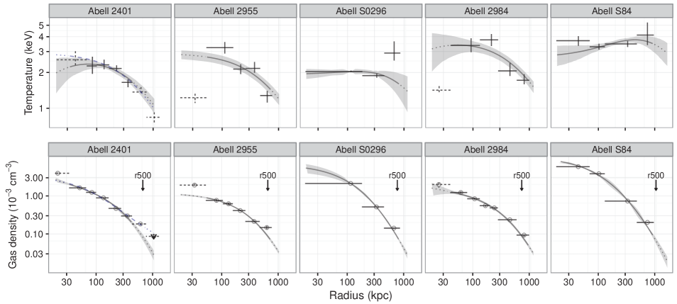
Figure 2: Gas temperature and density profiles for the clusters (error bars & hollow circles + error bars, respectively) with the best-fit AD08 cluster model (solid line) and 1$\sigma$ error envelope. Also shown, in columns 4 and 5, are two additional clusters included to increase the sample size, as described in section 2.3. The innermost bin was excluded from the fit in all cases and is plotted with dashed error bars. Dotted curves indicate extrapolation of the model beyond the data and the blue dashed curve for A2401 is the (much worse) best-fit model including the penultimate bin and with the polytropic index free to vary. Note that for A2401 the outermost bin is excluded in both cases and so the corresponding density point has not been corrected for projection and is plotted as an upper limit (see text for details).

The cluster model was jointly fitted to the deprojected gas density and temperature profiles, excluding the central bin, since our focus is on global properties and we expect complex baryon physics on the scale of the BCG to invalidate the model assumptions here; the fitted data and model are plotted in Fig. 2. To improve the radial coverage of the gas distribution, we also use the cluster model to determine a correction factor for estimating the density in the outermost bin. This point is often omitted on the basis that the emission in the outer annulus has not been deprojected and so includes a contribution from gas distributed along the line of sight beyond the radius of the corresponding spherical shell. However, we can use the cluster model to estimate what fraction of the total emission in this annulus originates from the corresponding spherical shell.

Cluster	$T_{0}$ (keV)	$t$	$a$ (kpc)	$\alpha$	$f$	$r_{\mathrm{500}}$ (kpc)	$r_{\mathrm{fit}}$ (kpc)	$\chi^{2}$ / dof	$p$ value	$f_{\rho}$	$f_{kT}$
Abell 2401	2.94 $\pm$ 0.25	0 $\pm$ 0.11	588 $\pm$ 135	0.01 $\pm$ 0.03	0.73 $\pm$ 0.18	672 $\pm$ 20	432	13.3/4	0.010	0.03	0.02
Abell 2955	2.9 $\pm$ 0.30	1 $\pm$ 0.00	709 $\pm$ 51	0.01 $\pm$ 0.01	0.78 $\pm$ 0.11	656 $\pm$ 32	770	13.0/4	0.011	0.01	0.13
Abell S0296	3.91 $\pm$ 0.38	0 $\pm$ 0.00	750 $\pm$ 125	0.01 $\pm$ 0.02	0.73 $\pm$ 0.12	772 $\pm$ 39	997	36.8/5	0.000	0.07	0.06
Abell 2984	3.72 $\pm$ 1.06	0.52 $\pm$ 0.16	870 $\pm$ 382	0.49 $\pm$ 0.48	0.30 $\pm$ 0.18	738 $\pm$ 66	861	10.6/1	0.001	0.00	0.23
Abell S84	7.69 $\pm$ 1.43	0.35 $\pm$ 0.07	1337 $\pm$ 337	0.38 $\pm$ 0.69	0.18 $\pm$ 0.08	1054 $\pm$ 85	963	52.4/3	0.000	0.06	0.06

Table 2: Best-fitting model parameters for each cluster and 1$\sigma$ errors estimated from 200 bootstrap resamples. $r_{\mathrm{fit}}$ is the radius of the outer annulus of the fitted data in the spectral profile. The last four columns are the $\chi^{2}$ / degrees of freedom with associated $p$ value and the mean fractional intrinsic scatter in the gas density and temperature, respectively (as defined in Sanderson & Ponman, 2010). The lower portion of the table refers to two additional clusters included to increase the sample size, as described in section 2.3.

To do this, we consider a line of sight column located at the half-radius of the spherical shell, and intersecting its outer edge at two points. The correction factor is simply the ratio of the density squared integrated along this line within the shell to that evaluated between $\pm$ infinity – this weighting approximates the emissivity of bremsstrahlung as well as that of low-temperature line emission. This fraction is then multiplied by the density obtained by assuming all the flux in the outer annulus is associated with the volume of the corresponding spherical shell. With the outer density point thus determined, a new best-fit model is obtained and used to evaluate a corresponding new estimate of the correction factor, until convergence is achieved. The final correction factors obtained are 0.70 for A2955 and 0.73 for AS0296. This then allows the outermost density point to be used in the analysis, albeit at the expense of introducing some model-dependency.

Cluster	$M_{2500}$ ($10^{14}M_{\sun}$)	$M_{500}$ ($10^{14}M_{\sun}$)	$r_{\mathrm{2500}}$ (kpc)	$r_{\mathrm{500}}$ (kpc)	$f_{\mathrm{gas}}$($<$$r_{\mathrm{2500}}$)	$f_{\mathrm{gas}}$($<$$r_{\mathrm{500}}$)	$\alpha^{a}$
Abell 2401	0.34 $\pm$ 0.05	0.91 $\pm$ 0.08	282 $\pm$ 15	672 $\pm$ 20	0.047 $\pm$ 0.003	0.073 $\pm$ 0.009	-0.48 $\pm$ 0.17
Abell 2955	0.28 $\pm$ 0.06	0.88 $\pm$ 0.13	260 $\pm$ 17	656 $\pm$ 32	0.036 $\pm$ 0.002	0.064 $\pm$ 0.005	-0.14 $\pm$ 0.01
Abell S0296	0.48 $\pm$ 0.12	1.4 $\pm$ 0.21	315 $\pm$ 27	772 $\pm$ 39	0.039 $\pm$ 0.003	0.065 $\pm$ 0.008	-0.29 $\pm$ 0.25
Abell 2984	0.37 $\pm$ 0.07	1.3 $\pm$ 0.35	286 $\pm$ 20	738 $\pm$ 66	0.087 $\pm$ 0.004	0.096 $\pm$ 0.014	-0.32 $\pm$ 0.10
Abell S84	1 $\pm$ 0.18	3.7 $\pm$ 0.96	399 $\pm$ 23	1054 $\pm$ 85	0.080 $\pm$ 0.015	0.075 $\pm$ 0.019	-0.47 $\pm$ 0.11

Table 3: Derived quantities from the cluster models with 1$\sigma$ errors estimated from 200 bootstrap resamples. ^aLogarithmic gradient of the gas density profile at 0.04$r_{\mathrm{500}}$ (after Vikhlinin et al., 2007); $\alpha\la-0.85$ indicates a strong cool core (Sanderson et al., 2009a). The lower portion of the table refers to two additional clusters included to increase the sample size, as described in section 2.3.

For A2401, the two outermost annular bins are only partially covered by the XMM-Newton CCD chips, as a result of the off-axis position of the cluster halo (see left panel of Fig. 1), resulting in systematically incomplete azimuthal coverage. For the outermost bin only 23 per cent of the annulus falls on the chip, while the penultimate bin has a coverage of 59 per cent. Recent work by Eckert et al. (2012) has found substantial azimuthal variation in ICM density in cluster outskirts, as a result of structural asymmetries and gas clumping, which could introduce significant systematic bias into the determination of the gas properties from incomplete outer annuli. Moreover, both of these bins include emission from beyond $r_{\mathrm{500}}$ and even beyond $r_{\mathrm{200}}$ for the outermost annulus, where the intracluster gas increasingly deviates from hydrostatic equilibrium (e.g Nagai et al., 2007) and may also be subject to complex physics like clumping (e.g. see Urban et al., 2011, and references therein), which would invalidate the model. We therefore exclude both the outer two bins from the fit and so are unable to determine a corrected density value for the outermost annulus, as this is model-dependent. However, since the uncorrected density represents an upper limit, we plot it in Fig. 2 with an arrow extending from the 1$\sigma$ upper bound.

The best-fit parameters for the final cluster models and their 1$\sigma$ errors (estimated from 500 bootstrap re-samples) are listed in Table 2, together with values of $r_{\mathrm{500}}$ and the radius of the outermost annular bin included in the fit. Following Sanderson & Ponman (2010), we consider the residual fractional intrinsic scatter of the gas density data about the model (which measures the real variance of the data about the model, beyond that expected from the measurement errors) as a useful indicator of the effectiveness of the model in describing the data (second last column of Table 2). This quantity is the mean value of $\left[(y_{obs}-y_{pred})^{2}-y_{err}^{2}\right]/y_{pred}$, with all negative values to zero, based on the observed values, predicted values and measurement errors of $y$ (see the appendix of Sanderson & Ponman, 2010). For A2401 and A2955 this scatter is three and one per cent, respectively, in gas density– well below the levels of $>$5 per cent associated with merging/disrupted clusters for which the model performs less well (Sanderson & Ponman, 2010). However, AS0296 has a 7 per cent residual intrinsic scatter in density, which hints at a somewhat irregular gas distribution which the model does not capture well. The fractional intrinsic scatter for the gas temperature is also presented in Table 2, although this is a less reliable diagnostic of model effectiveness (Sanderson & Ponman, 2010).

According to the best-fit models, none of these clusters hosts a sharply peaked cool core: the inner cuspiness as measured by the logarithmic slope of the gas density at 0.04$r_{\mathrm{500}}$ ($\alpha$, cf. Vikhlinin et al., 2007; Sanderson et al., 2009a) is flatter in all cases than the value of $\la-0.85$ which typically characterizes strong cool core clusters (Sanderson et al., 2009a, see Table 3). On the other hand, it is noticeable from Fig. 2 that the (excluded) innermost temperature point (radius $\la$ 40–50 kpc) lies substantially below the extrapolated model prediction in the cases of A2955 and AS0296. Our Ascasibar & Diego cluster model is fully able to describe cool cores (cf. Ascasibar & Diego, 2008; Sanderson & Ponman, 2010), but hydrostatic equilibrium is built into this model, and so deviations are expected on the scale of the central galaxy. In any case, the possible presence of small cool cores in these two clusters has no significant impact on the present study, which is concerned with the large scale properties of these systems.

2.3 Analysis of two extra poor clusters

In order to increase our coverage of the baryon fraction in groups/poor clusters for which a full intracluster light analysis has been performed, we have added two extra systems to our sample from a companion paper (Abell 2984 & Abell S84; Gonzalez et al., in preparation). These objects were also part of the GZZ07 sample and their XMM-Newton data were analysed in Sivanandam et al. (2009). For consistency, we have re-analysed these poor clusters in the same way as for our other three systems (i.e. as described in Sections 2.1 & 2.2), and their corresponding model parameters and derived quantities are listed in the lower portions of Tables 2 & 3 . The corresponding correction factors for determining the gas density in their outermost bins are 0.83 & 0.82 for A2984 & AS84, respectively. We address the comparison between our modelling analysis of these systems and that of Sivanandam et al. (2009) in Sections 5.3 & 5.4.

3 Optical data

Cluster membership was determined on the basis of galaxy velocities, which were obtained from dedicated spectroscopic (and associated photometric) observations in the case of A2955 and AS0296, yielding a total of 22 and 34 cluster members, respectively (Zaritsky et al., 2006) . These galaxies were originally selected for spectroscopic follow-up if they were both fainter than the BCG and located within a projected distance of 1.5 Mpc of it, and the resulting velocity distribution was subjected to a 3$\sigma$ clipping algorithm, to select the cluster members (Zaritsky et al., 2006), using biweight estimators of location and scale for improved robustness (Beers et al., 1990).

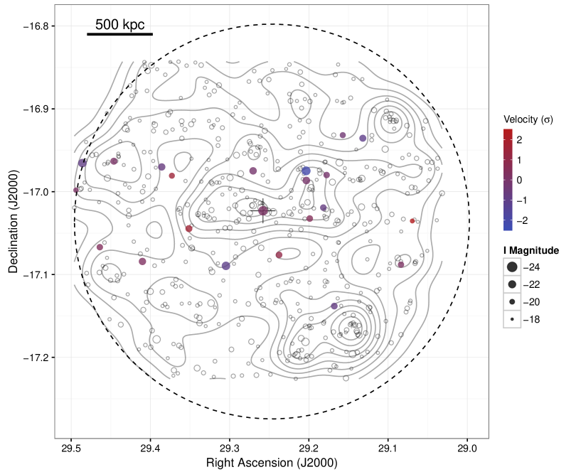
Figure 3: Positions of galaxies around Abell 2955 with corresponding isodensity contours superposed, Gaussian smoothed on a scale of 500 kpc. The point sizes indicate the $I$ band absolute magnitude (assuming all the galaxies are at the redshift of the cluster) and the filled points are the cluster members, coloured according to the velocity with respect to the cluster mean velocity, normalized by the velocity dispersion (see Table 4). The position of the brightest cluster galaxy is marked with a ‘+’ and the dashed circle marks the field-of-view of the corresponding XMM-Newton observation.

Cluster	$f_{\mathrm{star}}$($<$$r_{\mathrm{2500}}$)	$f_{\mathrm{star}}$($<$$r_{\mathrm{500}}$)	$f_{\mathrm{b}}$($<$$r_{\mathrm{2500}}$)	$f_{\mathrm{b}}$($<$$r_{\mathrm{500}}$)	$M_{500}$ ($\sigma$) ($10^{14}M_{\sun}$)	$\sigma$ (km/s)	Ngal	BM Type
Abell 2401	0.036 $\pm$ 0.006	0.028 $\pm$ 0.003	0.083 $\pm$ 0.006	0.101 $\pm$ 0.013	0.55	459${}_{-83}^{+101}$	24	II
Abell 2955	0.064 $\pm$ 0.013	0.034 $\pm$ 0.005	0.100 $\pm$ 0.006	0.098 $\pm$ 0.009	0.15	316${}_{-67}^{+85}$	22	II
Abell S0296	0.035 $\pm$ 0.009	0.019 $\pm$ 0.003	0.074 $\pm$ 0.007	0.085 $\pm$ 0.010	0.63	477${}_{-65}^{+76}$	34	I
Abell 2984	0.073 $\pm$ 0.014	0.031 $\pm$ 0.009	0.159 $\pm$ 0.008	0.127 $\pm$ 0.019	0.69	490${}_{-91}^{+112}$	29	I
Abell S84	0.035 $\pm$ 0.006	0.016 $\pm$ 0.004	0.115 $\pm$ 0.022	0.091 $\pm$ 0.023	0.85	522${}_{-122}^{+155}$	24	I

Table 4: Optically-derived data for the clusters. The last 4 columns are the optically-derived mass, velocity dispersion, number of galaxies with velocities and Bautz-Morgan type, repectively (from Zaritsky et al., 2006, GZZ07). The lower portion of the table refers to two additional clusters included to increase the sample size, as described in section 2.3.

The positions of galaxies are plotted in Figs. 3 & 4 with point size indicating their $I$ band absolute magnitude and with cluster members colour-coded according to their relative line-of-sight velocity (hollow points have unknown velocity). In addition, confirmed non-cluster members have been omitted– a total of 35 and 11 galaxies for A2955 and AS0296, respectively. Overlaid are contours of surface number density which were computed by kernel smoothing the positions of all the galaxies in the field with a Gaussian of bandwidth 500 kpc at the redshift of the cluster, using the task kde2d in the mass package (Venables & Ripley, 2002) in r. For A2401, galaxy velocities were extracted from the NASA Extragalactic Database (NED), giving a total of 24 cluster members. These were cross-matched with the 2 Micron All Sky Survey (2MASS) Extended Source Catalogue (XSC; Skrutskie et al., 2006) to provide $K$ band magnitudes and their positions are similarly plotted in colour in Fig. 5, together with those of other 2MASS XSC objects in the vicinity, for which the velocities are unknown (coloured in grey).

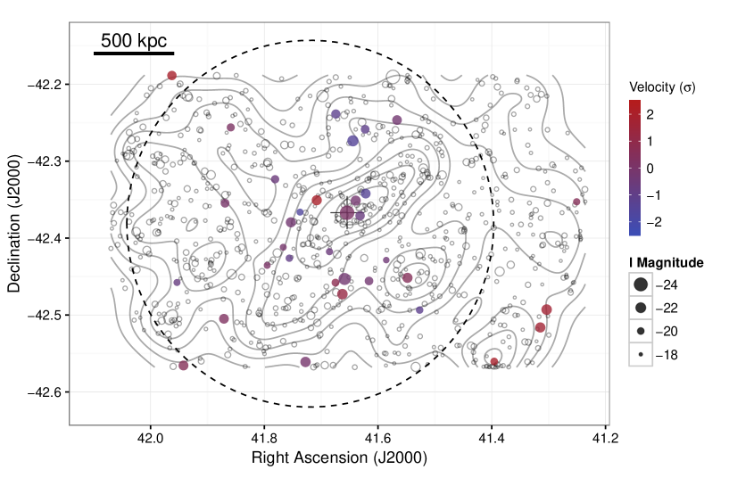
Figure 4: As for Fig. 3, but for Abell S0296.

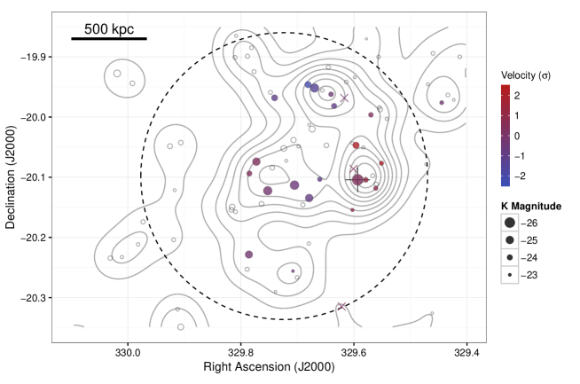
Figure 5: As for Fig. 3, but for Abell 2401 and using 2MASS $K$ band magnitudes. In this case the cluster members (filled, coloured points) were selected using data from the NED and the ‘$\times$’ symbols mark the positions of 3 galaxies with velocities but no corresponding $K$ magnitude.

In all cases the BCG lies very close to the peak of the number density contours smoothed on a scale of 500 kpc. However, other localized galaxy concentrations are evident, particularly in the case of A2401, which suggest either the presence of substructures in the cluster or ongoing merging/disruption. Moreover, the density contours are based on all the galaxies detected along the line of sight, not just those with redshifts and that were judged to be cluster members. Therefore, some of the features seen could be the result of unrelated fore- or background structures.

Fig. 6 shows the variation in line-of-sight velocity with distance from the BCG for galaxies spectroscopically confirmed to be members of the cluster. The behaviour seen is broadly consistent with the expected distribution for a virialized population of tracer particles, with no major anomalies that might cast doubt on the use of $\sigma$ as a mass estimator. For AS0296, there are four galaxies in the top right corner of the plot which are likely to be interlopers lying outside the virialized volume of the cluster; indeed 3 of these are visible as a clump of red dots in the lower right corner of the galaxy distribution plot in Fig. 4, suggesting an infalling substructure. However, their impact on the overall velocity dispersion of the cluster is minor and excluding their contribution would only further exacerbate the mass discrepancy compared to the larger X-ray determined value, discussed in Section 5.1. A2401 may also be affected by one or two interlopers, on the basis of Fig. 6, but here also any bias is likely to be small.

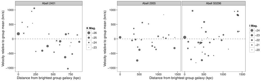
Figure 6: Line-of-sight velocity vs. distance from the brightest cluster galaxy for the galaxies spectroscopically confirmed as cluster members, point size coded by absolute magnitude. For Abell 2401, ‘$\times$’ symbols mark the positions of 3 galaxies with velocities but no corresponding $K$ magnitude.

We performed several tests of normality of the galaxy velocity distribution, using the r package nortest (e.g. Thode, 2002). For all three clusters, none of the tests appropriate for these sample sizes shows evidence for a non-Gaussian distribution, including the Anderson-Darling test, which has been shown to be the most sensitive to optical cluster substructure (Hou et al., 2009).

A key element in determining the stellar mass in clusters is the aperture within which the measurement is made, which depends on the total gravitating mass. In the original GZZ07 analysis, X-ray data were generally not available and so the total mass (within $r_{\mathrm{500}}$) was estimated from the velocity dispersion of the galaxies, using the relation between $\sigma$ and $M_{\mathrm{500}}$ based on the cluster sample of Vikhlinin et al. (2006), where a full hydrostatic mass analysis was performed. There is evidence that $\sigma$ can often underestimate the total mass in galaxy groups (Osmond & Ponman, 2004; Connelly et al., 2012), and so a key aim of the present study is to determine the mass independently, using our X-ray data. Indeed, as shown by Balogh et al. (2008), the four lowest mass GZZ07 clusters, including A2955 from our study, have uncomfortably high baryon fractions (implying an underestimated total mass) on the basis of their velocity dispersions-derived masses. However, these systems had been excluded by GZZ07 on the grounds that their mass estimates required an extrapolation of the $M_{\mathrm{500}}-\sigma$ relation and were hence unreliable (we emphasize that they were not excluded on the basis of $f_{\mathrm{b}}$). We address the differences between the X-ray and optically derived mass estimates in Section 5.1.

3.1 Intracluster light and stellar mass

GZZ07 made drift-scan observations to measure the optical light profile of the clusters, with accurately measured background and flat-fields, in order to map the diffuse ICL directly and with good precision in each case. The cluster radial light profile was modelled as a combination of two de Vaucouleurs profiles, to capture the separate contributions from the BCG and ICL. The total optical luminosity of the cluster is calculated by integrating the model within a given aperture and then adding in the luminosities of the individual non-BCG cluster galaxies in the same aperture (corrected for contamination). Since our X-ray derived masses (Table 3) are substantially larger than the masses derived from velocity dispersions by GZZ07, as we will discuss in Section 5.1, the apertures corresponding to $r_{\mathrm{2500}}$ and $r_{\mathrm{500}}$, within which the optical luminosity are integrated are correspondingly larger. We therefore re-measured the cluster optical luminosity (including ICL) within these new radii.

These aperture measurements represent the projected luminosity within a cylinder along the line of sight through the cluster. We have therefore corrected them for projection, to calculate the 3 dimensional luminosity within a sphere, assuming a Navarro et al. (1995) profile with a concentration parameter of 2.9 (based on the stacked profile of Lin et al., 2004). This correction only applies to the galaxy distribution and not the BCG+ICL light, which is (approximately) completely contained within the smallest aperture considered here ($r_{\mathrm{2500}}$). The ratios of the deprojected to projected luminosities are in the range 0.74–0.91 within $r_{\mathrm{2500}}$ and 0.78–0.86 within $r_{\mathrm{500}}$.

Our adopted average $I$ band mass to light ratio (M/L) is 2.65, which is lower than that used in GZZ07. This new value incorporates a 15 per cent contribution from dark matter as well as a correction to the previous GZZ07 M/L calculation which is described in more detail in a forthcoming paper (Gonzalez et al, in preparation). The corresponding stellar masses and mass fractions are summarized in Table 4, together with other optical data for the 5 clusters. In Section 5.5 we address the impact on our results of systematic errors in M/L.

4 Results

4.1 Radial trends in stellar and gas fraction

The radial distribution of baryonic components is plotted in Fig. 7, with the WMAP7 inferred Universal baryon fraction shown for comparison. The gas fraction from the cluster model is plotted as a solid curve with grey error envelope, with dots indicating extrapolation beyond the data. Aperture values of the stellar mass fraction (including the ICL) are plotted at $r_{\mathrm{2500}}$ and $r_{\mathrm{500}}$, with corresponding total baryon fraction (gas + stars) plotted at the same radii. It can be seen that for all 5 clusters the stellar fraction is higher within $r_{\mathrm{2500}}$ than $r_{\mathrm{500}}$, although this difference is not statistically significant for A2401. This is also consistent with the observation that the ICL in these systems is more spatially concentrated than the galaxies themselves (GZZ07), as also found in the SDSS stacking analysis of Zibetti et al. (2005), for example. On the other hand, the gas fraction profiles tend to increase monotonically with radius, with the exception of AS84 and A2984, in accordance with the tendency for the intracluster medium to be more extended than the dark matter (e.g. David et al., 1995; Sanderson et al., 2003; Vikhlinin et al., 2006; Sun et al., 2009). Interestingly, the nearly flat $f_{\mathrm{gas}}$ profiles and more centrally-concentrated $f_{\mathrm{star}}$ for AS84 and A2984 imply a decline in total baryon content with radius. However, this difference is not significant for AS84 and, for A2984, $f_{\mathrm{b}}$ within $r_{\mathrm{500}}$ is only 1.7$\sigma$ lower than $f_{\mathrm{b}}$ within $r_{\mathrm{2500}}$.

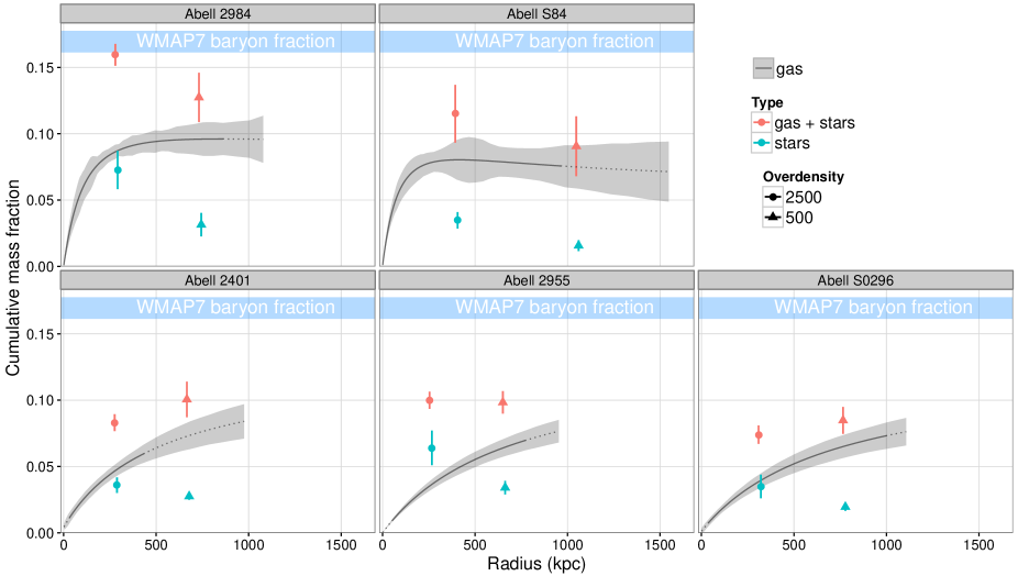
Figure 7: Gas mass fraction profiles plotted out to $r_{\mathrm{200}}$ for each cluster, with the stellar and total baryon fraction (including ICL) evaluated at $r_{\mathrm{500}}$ and $r_{\mathrm{2500}}$ (offset slightly in radius to avoid over plotting). The grey region is the 1$\sigma$ confidence envelope on the gas fraction profile from the cluster model and a dotted curve denotes extrapolation of the model beyond the radius of the outermost bin (see Table 2).

The mass fractions for the baryon components averaged over all 5 poor clusters are listed in Table 5, measured within $r_{\mathrm{2500}}$ and $r_{\mathrm{500}}$ and weighted by the inverse squared measurement errors. The calculation was performed in log space since the baryon fraction is right skewed, as a consequence of being strictly bounded by zero below. This is confirmed by the fact that a log-normal distribution provides a better description of the data than a normal distribution (as determined using the fitdistr function in the mass package in r; Venables & Ripley, 2002). It can be seen that the combined baryon fraction within the two radii does not significantly differ, reaching a value of $0.096\pm 0.006$ within $r_{\mathrm{500}}$ (at the corresponding mean $M_{\mathrm{500}}$ of $(1.08^{+0.21}_{-0.18})\times 10^{14}M_{\sun}$), and falls some way short (reaching only 57 per cent) of the Universal mean level of $0.169\pm 0.008$ from WMAP7 (Jarosik et al., 2011). On the other hand the balance of hot and cold baryons does vary radially, with the ratio of stellar to total baryon mass declining from 0.44 to 0.27 between $r_{\mathrm{2500}}$ and $r_{\mathrm{500}}$.

Looking at Fig. 7, if we consider only the systems where the fitted data extend beyond $r_{\mathrm{500}}$ (i.e. where no extrapolation is required), it is clear that a substantial baryon deficit is present in two of three cases, and is a factor of $\sim$2 for AS0296 (with a best-fitting value of $50\pm 6$ per cent of the Universal mean); for A2984, $f_{\mathrm{b}}=0.127\pm 0.019$, representing $75\pm 11$ per cent of the Universal mean $f_{\mathrm{b}}$. We demonstrate in Section 5.6 that, for 4/5 cases, the baryon fractions cannot be reconciled with the Universal mean even when conservatively accounting for systematic errors.

	$r_{\mathrm{2500}}$	$r_{\mathrm{500}}$
$f_{\mathrm{star}}$	0.0450${}_{-0.0067}^{+0.0078}$	0.0261${}_{-0.0028}^{+0.0031}$
$f_{\mathrm{gas}}$	0.0580${}_{-0.0105}^{+0.0128}$	0.0702${}_{-0.0046}^{+0.0050}$
$f_{\mathrm{gas+stars}}$	0.1030${}_{-0.0124}^{+0.0150}$	0.0963${}_{-0.0054}^{+0.0058}$
Mtot ($10^{13}$ M☉)	4.43${}_{-0.94}^{+1.19}$	10.83${}_{-1.76}^{+2.10}$

Table 5: Weighted mean mass fractions for the baryon components and total mass, measured within $r_{\mathrm{500}}$ and $r_{\mathrm{2500}}$. The calculation was performed in log space, yielding an asymmetric standard error on the unlogged values.

4.2 Variation in stellar and gas fraction

With our new X-ray derived total masses and the associated overdensity radii, we are able to address one of the key results of GZZ07, namely the stellar mass fraction in poor clusters. The left panel of Fig. 8 shows $f_{\mathrm{star}}$ vs. $M_{500}$ for these 5 clusters. Also plotted, as dotted error bars, are the positions of 4 of the clusters from the original GZZ07 analysis (the A2955 $f_{\mathrm{star}}$ measurement was excluded from that analysis, since its mass estimate was deemed unreliable, being based on an extrapolation of the $M_{\mathrm{500}}$ - $\sigma$ relation). It is clear that the new positions for these points are substantially different, primarily due to the X-ray masses being considerably larger than those derived from the velocity dispersion, which we discuss further in Section 5.1.

The larger masses result in a larger $r_{\mathrm{500}}$ aperture within which $f_{\mathrm{star}}$ is measured and, since the BCG and ICL stellar contribution falls off rapidly with radius (Section 4.1), the result is a lower stellar fraction. However, it is interesting that the change in both quantities acts to move the points mostly along the regression line, thus largely preserving the trend found by GZZ07. While this is not altogether surprising given the covariance between $f_{\mathrm{star}}$ and $M_{\mathrm{500}}$ (since $f_{\mathrm{star}}\propto M_{\mathrm{500}}^{-1}$), the shift is nevertheless along a flatter trajectory than implied by the relation between these quantities. For reference, the dashed line in the left panel of Fig. 8 shows the best fitting orthogonal regression from an analysis of new observations of the (optically selected) GZZ07 sample (Gonzalez et al, in preparation), which incorporates the results from this work. Despite the substantial change in total mass and a reduction in the measurement errors, the five clusters remain fairly consistent with the trend and scatter in the $f_{\mathrm{star}}$ – $M_{\mathrm{500}}$ relation from GZZ07.

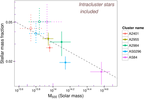
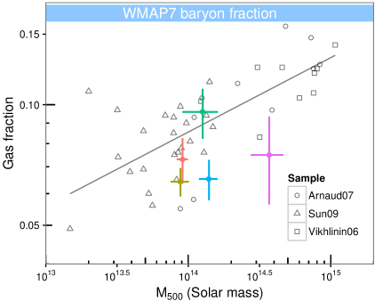
Figure 8: Left: Stellar mass fraction (including intracluster stars) vs. cluster total mass within $r_{\mathrm{500}}$, updating the results from GZZ07 (dotted error bars, which were not corrected for projection) with X-ray derived data from this work (solid error bars). The dashed line is the best fitting orthogonal regression from an analysis of new observations of the GZZ07 sample (Gonzalez et al, in preparation). This sample includes the five clusters from this work, but mainly comprises more massive clusters. Note that A2955 was excluded from the original plot data of GZZ07, but would have been located off the left hand edge of the plot, and that an $I$ band mass-to-light ratio of 2.65 is used to calculate stellar mass (see Section 3.1 further details). Right: gas fraction vs. mass for the same 5 clusters, together with X-ray selected data from the literature (Vikhlinin et al., 2006; Arnaud et al., 2007; Sun et al., 2009). The solid line is the best-fitting BCES power law regression to the X-ray selected literature data only (i.e. excluding our 5 clusters), with logarithmic slope of $0.186\pm 0.083$.

The corresponding relationship between gas fraction and mass is plotted in the right panel of Fig. 8. For comparison, data from the X-ray selected cluster samples of Vikhlinin et al. (2006) and Arnaud et al. (2007) as well as the X-ray selected groups sample of Sun et al. (2009) are also shown, with error bars omitted for clarity. The solid line is the best-fitting BCES orthogonal regression (Akritas & Bershady, 1996) in log-log space, which excludes our 5 clusters and thus represents a purely X-ray selected sample. Of the 5 clusters, only A2984 is located near the trend, with the remaining 4 all lying near the lower edge of the scatter about the fit, in contrast to the $f_{\mathrm{star}}$ – $M_{\mathrm{500}}$ relation. This is not necessarily surprising, since these were not X-ray selected clusters and therefore might be expected to have lower $f_{\mathrm{gas}}$ (and hence $L_{\mathrm{X}}$), as seen in other optically-selected groups and clusters (e.g. Bower et al., 1997; Rasmussen et al., 2006; Rykoff et al., 2008a; Hicks et al., 2008; Dai et al., 2010; Balogh et al., 2011). Indeed, Rykoff et al. (2008b) demonstrate that differences in the X-ray luminosity–total mass relation between optically and X-ray selected cluster samples can be at least partly explained by the combination of Malmquist bias and deviations from hydrostatic equilibrium affecting the latter.

4.3 Variation in total baryon content

The sums of the stellar (including ICL) and gas fractions within $r_{\mathrm{500}}$ for the five clusters are plotted in Fig. 9, to show the variation in total baryon content compared to the Universal mean fraction. Fractional errors on the total baryon fraction were calculated by adding in quadrature the fractional errors on the gas and stellar fractions. Also indicated in Fig. 9 is the level of a 10 per cent depleted Universal $f_{\mathrm{b}}$ (i.e. 0.9$\times\Omega_{b}/\Omega_{m}$ hereafter referred to as the ‘depleted cosmic’ $f_{\mathrm{b}}$), representing the typical value seen within $r_{\mathrm{500}}$ in simulated clusters (e.g. Ettori et al., 2006). It can be seen that 4 out of 5 of our (optically-selected) clusters fall significantly ($>2\sigma$) below this line, implying a baryon deficit. With the exception of A2984, this is mainly the result of a low gas fraction compared to the trend (right panel Fig. 8), although A2984 lies close to the trend in both gas and stellar fraction but still shows evidence of baryon shortfall. Furthermore, even when allowance is made for systematic uncertainties, these baryon fractions cannot be reconciled with the Universal mean (see Section 5.6).

5 Discussion

An important aspect of our findings is that the X-ray determined masses of the 5 clusters are all substantially greater than implied by the velocity dispersion of their galaxy members. Therefore, in this section we first address this issue, before turning to a discussion of potential systematic effects relating to the gas and stellar mass measurements and finally considering the interpretation of our results and their associated implications.

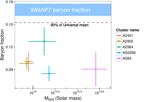
Figure 9: Total baryon fraction (hot gas + stars) vs. total mass within $r_{\mathrm{500}}$ for the 5 clusters. The horizontal dashed line shows the ‘depleted cosmic’ $f_{\mathrm{b}}$ typically expected within $r_{\mathrm{500}}$ from simulations without radiative cooling or feedback (e.g. Ettori et al., 2006).

5.1 X-ray vs. optical mass estimates

Estimating the gravitating mass of galaxy clusters is crucial in two ways in determining their baryon fraction, since this enters as the denominator in that quantity as well as determining the aperture within which the measurement is made. The original GZZ07 analysis used the optical velocity dispersion of the galaxies to estimate M₅₀₀ (via the $M-T_{\mathrm{X}}$ and $\sigma-T_{\mathrm{X}}$ scaling relations) and this quantity is plotted in Fig. 10 against the corresponding X-ray inferred value measured in this work, with the locus of equality indicated. In all cases the X-ray estimates are significantly higher than their optical counterparts, by a factor of between 1.7 and 5.7 (mean 3.1).

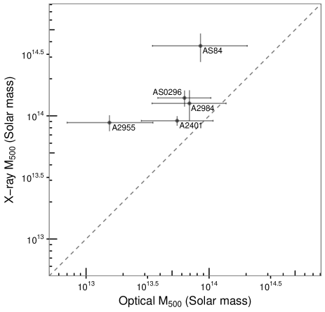
Figure 10: A comparison of M₅₀₀ as measured from X-ray data in this work with the optically-derived estimates in GZZ07, which were based on the velocity dispersion of galaxies in the cluster and an assumed $\sigma$-$M_{\mathrm{500}}$ relation. The dashed line shows the locus of equality.

Part of the discrepancy can be attributed to the calibration of the $M-\sigma$ used by GZZ07, which was necessarily limited by the lack of clusters with suitably well measured masses and velocity dispersions. However, other potential causes of such a discrepancy are failures of one or both of the two key assumptions in both X-ray and optical mass estimates, namely equilibrium and spherical geometry. On the X-ray side, non-thermal pressure support and/or deviations from hydrostatic equilibrium (e.g. due to recent disruption) are expected to cause X-ray mass underestimates of $\sim$5–20 per cent (e.g. Kay et al., 2004; Rasia et al., 2006; Nagai et al., 2007; Piffaretti & Valdarnini, 2008); accounting for this effect would only exacerbate the disagreement in this case. Nevertheless, deviations from hydrostatic equilibrium are likely to contribute towards the scatter in X-ray mass estimates, for which we make allowance in our analysis of the systematic error budget in Section 5.5.

With the exception of A2984 (where the uncertainties are large), none of the clusters hosts a strong cool core (see Table 3), the absence of which is often associated with recent disruption (e.g. Sanderson et al., 2006). On the other hand, there is no indication of any significant offset between the X-ray peak/centroid and the BCG, which suggests a lack of disturbance (Sanderson et al., 2009a). Moreover, since these are optically selected clusters, it is plausible that they may have a lower incidence of cool cores compared to X-ray selected samples, since the presence of a cool core invariably boosts the X-ray flux in the region of highest surface brightness.

Another possible explanation is that the line-of-sight velocity dispersion is systematically underestimated for these clusters, which could occur if the cluster was substantially elongated in the plane of the sky. This hypothesis is difficult to test, given the limited number of member galaxies, but the morphology of the isodensity contours of all the surrounding galaxies (which includes fore- and background objects as well as cluster members) hints at such a possible elongation in the case of A2955 (Fig. 3) and AS0296 (Fig. 4). No such elongation is evident for A2401 (Fig. 5), and here the optical and X-ray masses are in better agreement (although still significantly discrepant). Interestingly, Connelly et al. (2012) have found that dynamical masses have a large scatter and, for less massive clusters in particular, are biased low compared to X-ray mass estimates. This suggests that, for poor clusters in general, X-ray mass estimates may be more reliable than those based on the velocity dispersion of the member galaxies, particularly when the number of galaxies is relatively small ($\sim$20–30; Table 4). Indeed, Biviano et al. (2006) find that the scatter in $\sigma$-based mass estimates roughly doubles when the number of galaxies decreases from $\sim$400 to $\sim$20 (reaching $\sim$0.6 for $N_{\mathrm{gal}}$=10), based on an analysis of 62 simulated clusters. However, this alone is not sufficient to account for the discrepancy in this case, which amounts to a systematic bias of at least a factor of $\sim$2.

5.2 The impact of the total mass on $f_{\mathrm{b}}$

The total gravitating mass determines the aperture for measuring the gas and stellar masses, via the definition of an overdensity, $\Delta$, with respect to the redshift-dependent critical density of the Universe, $\rho_{\mathrm{crit}}(z)$

$$M_{\Delta}=\Delta\,\frac{4}{3}\pi\,r^{3}_{\Delta}\,\rho_{\mathrm{crit}}(z)\,.$$ (2)

The stellar and gas fractions are inversely proportional to $M_{\Delta}$, by definition, and in general both vary oppositely with radius (Fig. 7). As a result, $f_{\mathrm{b}}$ within a given overdensity radius, $r_{\Delta}$, depends quite subtly on the corresponding $M_{\Delta}$, via Equation 2. Thus a large change in $M_{\mathrm{500}}$ does not necessarily change the baryon fraction within $r_{\mathrm{500}}$ substantially. As a consequence, $f_{\mathrm{b}}$ is quite robust to variations in $M_{\mathrm{500}}$ resulting from modelling uncertainties, for example.

The sensitivity of the baryon fraction measured within $r_{\mathrm{500}}$ to the assumed $M_{\mathrm{500}}$ can be judged by exploring the effect of artificially altering the value of $r_{\mathrm{500}}$, as follows. The gas and stellar masses are measured within each nominal value of $r_{\mathrm{500}}$ and the corresponding $f_{\mathrm{b}}$ is calculated by adding them together and dividing by the $M_{\mathrm{500}}$ calculated from Equation 2. The stellar mass is calculated from $f_{\mathrm{star}}$, which is fixed at the spot values for $r_{\mathrm{2500}}$ and $r_{\mathrm{500}}$ for $r\leq r_{\mathrm{2500}}$ and $r\geq r_{\mathrm{500}}$, respectively, and linearly interpolated in log-log space in between. Fig. 11 shows curves of the resulting implied baryon fraction measured in this way within each nominal $r_{\mathrm{500}}$ aperture.

Under the hypothesis that the true $f_{\mathrm{b}}$ is 15 per cent (roughly the ‘depleted cosmic’ $f_{\mathrm{b}}$ level of 0.9 times the Universal mean), the corresponding $r_{\mathrm{500}}$ required to achieve this result is plotted as a dashed vertical line in Fig. 11. For comparison, the observed $r_{\mathrm{500}}$ is shown as a dotted line and ratios of the implied $M_{\mathrm{500}}$ and $r_{\mathrm{500}}$ to their observed counterparts are shown in the strip titles for each panel in the plot. With the exception of A2984, the masses would need to have been overestimated by $\sim$ 2–4 times to achieve $f_{\mathrm{b}}=0.15$, equivalent to an overestimate in mean temperature of $\sim$1.3–2.7 times. Thus the observed deficiency of baryons can only be accounted for by a factor of $\sim$ 2–4 systematic error in the determination of the total mass. Such a large error greatly exceeds both the measurement errors and our best estimate of the true systematic uncertainty, as we demonstrate in Section 5.3.

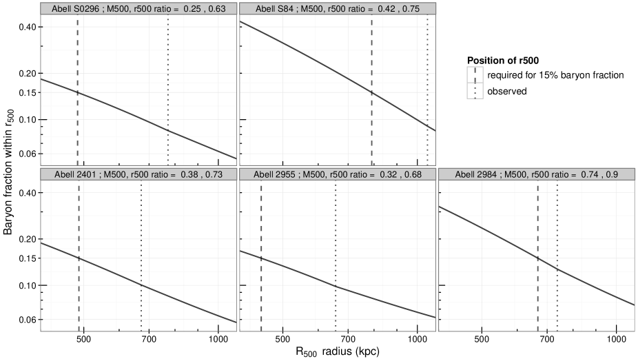
Figure 11: Baryon fraction profiles implied by assuming that each radius corresponds to $r_{\mathrm{500}}$, with dashed vertical lines marking the radius required to achieve a nominal ‘depleted cosmic’ value of $f_{\mathrm{b}}=0.15$ within $r_{\mathrm{500}}$, as compared to the position of the observed value of $r_{\mathrm{500}}$ (dotted lines). Ratios of the implied $M_{\mathrm{500}}$ and $r_{\mathrm{500}}$ for the case of $f_{\mathrm{b}}=0.15$ to the corresponding observed values are indicated in the strip text for each panel. See text for details.

5.3 Cross-check of X-ray masses using the $M-T_{\mathrm{X}}$ relation

To test the accuracy of the masses determined from the cluster modelling, we also estimated $M_{\mathrm{500}}$ from the mass-temperature ($M-T_{\mathrm{X}}$) relation of Vikhlinin et al. (2006), based on a global mean temperature ($\overline{T}$). We estimated $\overline{T}$ using $\rho_{\mathrm{gas}}$$(r)$ and $T(r)$ from the best-fitting cluster model, evaluating a weighted (by $\rho^{2}_{\mathrm{gas}}\sqrt{T}$) mean in the radial range (0.15–1) $r_{\mathrm{500}}$, determined iteratively (since $r_{\mathrm{500}}$ depends on $M_{\mathrm{500}}$, which depends on $\overline{T}$). The comparison between $M_{\mathrm{500}}$ calculated by these two methods is plotted in Fig. 12, which shows good agreement in all cases and no indication of any systematic bias. This is consistent with the good agreement in $r_{\mathrm{500}}$ found by Sanderson & Ponman (2010) between the AD08 cluster model and the Vikhlinin et al. $M-T_{\mathrm{X}}$ relation, using direct extraction and fitting of spectra in an iteratively adjusted aperture (from Sanderson et al., 2009b). Although the $M-T_{\mathrm{X}}$ masses estimated in this way are not completely independent from the AD08 model masses, this comparison nevertheless demonstrates consistency between both the two methods and the cluster samples, in respect of hydrostatic equilibrium. Since the Vikhlinin et al. clusters were carefully selected to have very regular X-ray morphology and with only weak signs, if any, of dynamical activity, it is therefore reasonable to infer that our cluster model-derived X-ray mass estimates are reliable and not substantially affected by any departures from hydrostatic equilibrium and/or spherical symmetry within the hot gas haloes of the five clusters.

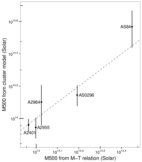
Figure 12: A comparison of M₅₀₀ determined from the cluster model with that estimated from the $M-T_{\mathrm{X}}$ relation of Vikhlinin et al. (2006). The dashed line shows the locus of equality.

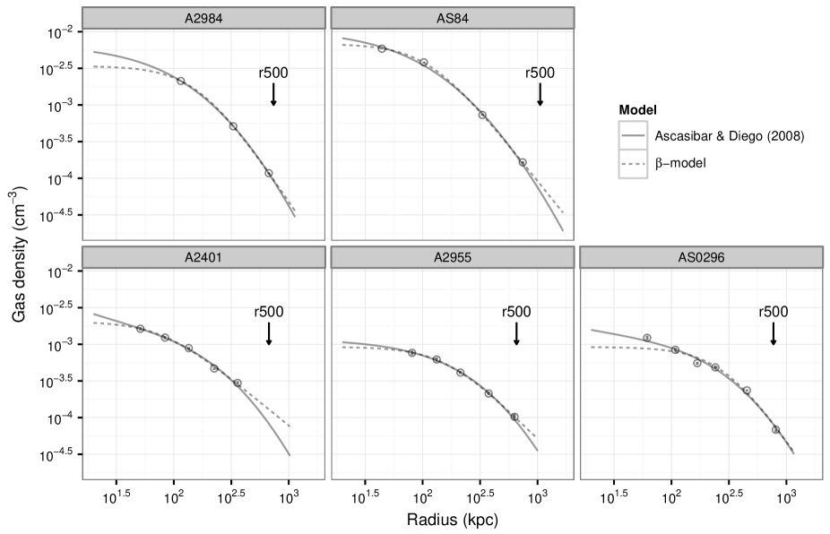
Figure 13: A comparison of the best-fitting AD08 and $\beta$-model gas density profiles, with the measured data plotted as hollow points and (mostly very small) error bars. Within each panel the profiles extend out to $r_{\mathrm{200}}$. For A2401, the excluded outermost two points (see Section 2.2) are not shown, but both lie above the best-fit $\beta$-model.

A further comparison of the total cluster mass is available for A2984 & AS84 from the independent analysis of the same XMM-Newton data by Sivanandam et al. (2009), also using the Vikhlinin et al. (2006) $M-T_{\mathrm{X}}$ relation, but measuring the mean temperature directly via spectral fitting of the raw data. The values of $M_{\mathrm{500}}$ obtained by Sivanandam et al. are (in units of $10^{14}$ M_⊙) $0.96\pm 0.098$ for A2984 (compared to $1.3\pm 0.35$; Table 3) and $2.6\pm 0.28$ for AS84 (compared to $3.7\pm 0.96$; Table 3). In both cases our masses are $\sim$1.4 times larger (albeit consistent to within the statistical uncertainties), which places an upper bound on uncertainties associated with the approach employed. As a result, we conclude that our X-ray derived mass estimates (and corresponding $r_{\mathrm{500}}$ and $r_{\mathrm{2500}}$ apertures) are reliable and that their measurement errors capture all reasonable sources of uncertainty. However, the impact of the mass measurement method is incorporated into our estimate of the systematic error on gas fraction at the end of Section 5.4. The main reason for the systematic difference in our masses compared to those of Sivanandam et al. is a difference in the steepness of the outer gas density profile, which directly affects the pressure gradient and hence the enclosed hydrostatic mass, and we investigate this issue further in the next section.

5.4 Choice of gas density model

It is noteworthy that the issue of the gas density in the outer regions of galaxy groups and poor clusters is not well explored, but it is clearly of importance in measuring the gas mass. It is now well established that in more massive clusters the density profile beyond $\ga$ 0.5 $r_{\mathrm{500}}$ typically steepens relative to a power law extrapolated from smaller radii (i.e. a $\beta$-model), from studies with Rosat (Vikhlinin et al., 1999), XMM-Newton (Croston et al., 2008) and Chandra (e.g. Ettori & Balestra, 2009). However, no such steepening has been found in galaxy groups, where a $\beta$-model provides a good description of the density profile out to $r_{\mathrm{500}}$ (Rasmussen & Ponman, 2004). We therefore also fitted $\beta$-models to the deprojected data points for all 5 clusters to cross-check the results from the AD08 cluster model, which does not use a $\beta$-model for the gas density profile. The comparison is made in Fig. 13 and it is clear that for A2955, AS0296 & A2984 there is excellent agreement between the two different models. Moreover, in each of these cases the data extend beyond $r_{\mathrm{500}}$, resulting in negligible differences in the gas mass within $r_{\mathrm{500}}$ ($\la$ 3 per cent) between the two models. Beyond this radius the models tend to diverge, which reflects the lack of data points to anchor the fit, while differences between the two models inside of the innermost data point reflect the inability of the (flat cored) $\beta$-model to capture the modest cuspiness in the density profiles.

In making this comparison, it should be noted firstly that the AD08 model is jointly fitted to both $\rho_{\mathrm{gas}}$$(r)$ and $T(r)$, assuming hydrostatic equilibrium and, also, that the AD08 model gas density profile is somewhat similar to a $\beta$-model in the limit where there is no cool core component (see figure 1 of AD08) – corresponding to $t=1$, which is the case for A2955 (see Table 2 ). Furthermore, the AD08 model assumes a polytropic ICM, which may not represent the true physical state of the gas, although this assumption does not apply within the cool core (if one is present– i.e. $t<1$ in Table 2). In the case of A2401 there is a difference between the extrapolated model profiles beyond the outermost data point, with the AD08 model steepening compared to the $\beta$-model and yielding a lower gas mass within $r_{\mathrm{500}}$ by 15 per cent. On the other hand, the two gas mass estimates agree to within 5 per cent for AS84, where extrapolation is also needed to reach $r_{\mathrm{500}}$.

It is clear from the 3 clusters with the best radial data coverage (A2984, A2955 & AS0296; Fig. 13) that no steepening of the gas density profile logarithmic slope is observed, within at least $r_{\mathrm{500}}$. This is quite different from the trend in more massive clusters and we discuss the implications of this behaviour in Section 5.7. However, our results are in accordance with Rasmussen & Ponman (2004), who found that $\rho_{\mathrm{gas}}$$(r)$ was well described by a $\beta$-model over the entire radial range (which extended beyond $\sim$$r_{\mathrm{500}}$) in two galaxy clusters of a similar mass scale ($\sim$2 kev). On the other hand, Sun et al. (2009) claim that the Vikhlinin et al. (2006) $\rho_{\mathrm{gas}}$$(r)$ model (which features a steepening logarithmic gradient) provides a good fit to their Chandra sample of 43 galaxy groups (although a number of these systems are not well covered azimuthally and/or radially beyond $\sim$0.5$r_{\mathrm{500}}$).

Finally, as was the case with the total mass, we are also able to perform a cross-check of our gas mass results for A2985 and AS84, for which the same XMM-Newton data were analysed by Sivanandam et al. (2009), using a different analysis and modelling approach. They generated XMM-Newton MOS X-ray surface brightness images, with corresponding exposure maps and background images and fitted these with a two-dimensional $\beta$-model, convolved with the instrument point spread function. They then deprojected this fitted profile using the Abel transform, and applied a global spectral fit to determine the corresponding normalization in terms of gas density. The values of $M_{\mathrm{gas}}$ ($<$ $r_{\mathrm{500}}$) obtained by Sivanandam et al. are (in units of $10^{13}$ M_⊙) $1.1\pm 0.08$ for A2984 (compared to $1.21\pm 0.15$; based on the data shown in Table 3) and $2.3\pm 0.13$ for AS84 (compared to $2.77\pm 0.61$; Table 3), which are not significantly different from our own measurements.

Although our estimates of the separate systematic effects of total and gas mass measurement method are not substantially different from zero, they compound in the measurement of the gas fraction. Our best estimate of the systematic error in measuring $f_{\mathrm{gas}}$ can be obtained from a comparison of our results with those of Sivanandam et al. (2009), who used different methods to us for determining both the total and gas mass (albeit applied to the same XMM-Newton data). The ratios of $f_{\mathrm{gas}}$ within $r_{\mathrm{500}}$ measured with the AD08 model vs. Sivanandam et al. method are $0.83\pm 0.17$ and $0.85\pm 0.26$ (for A2984 & AS84, respectively, with fractional errors summed in quadrature). While neither of these ratios is significantly different from 1, they are quite similar and somewhat less than one. Taking our AD08 model results as a baseline, this represents a systematic increase of 15 per cent in $f_{\mathrm{gas}}$ as a result of using a different analysis method. We therefore assign a systematic uncertainty of +15 per cent associated with the deprojection analysis and cluster modelling, but acting only in the direction of increasing $f_{\mathrm{gas}}$. This and the other contributions to the systematic error budget for the gas fraction are summarised in the middle column of Table 6, with negative values quantifying any potential decrease in $f_{\mathrm{gas}}$ with respect to our baseline model.

5.5 Other systematic effects

The bootstrap re-sampling approach, used to evaluate uncertainties on all quantities derived from the cluster model, yields a direct estimate of the statistical error that takes full account of intrinsic correlations (e.g between the gas and total mass in calculating $f_{\mathrm{gas}}$) and avoids the need for error propagation. However, it is important to consider sources of systematic uncertainty that could bias our results in a way that is not captured by these measurement errors.

As already mentioned in Section 2.2, one source of systematic error is gas clumping (e.g. Urban et al., 2011; Nagai & Lau, 2011, and references therein), which acts to bias the gas density higher. Since it is more prevalent in cluster outskirts, clumping would lead to a flatter density profile and a correspondingly overestimated gas mass and $f_{\mathrm{gas}}$, although this is difficult to quantify. In a similar fashion, non-thermal pressure support or merger-driven deviations from hydrostatic equilibrium could lead to an overestimated gas fraction, by $\sim$5–20 per cent – the amount by which the total mass is likely underestimated (e.g. Kay et al., 2004; Rasia et al., 2006; Nagai et al., 2007; Piffaretti & Valdarnini, 2008). In any case, both these phenomena would lead to problems in fitting the AD08 cluster model and likely result in a discrepant gas mass compared to that estimated from a surface brightness deprojection, using a $\beta$-model for example. While we cannot rule this out, the indications from Section 5.4 are that any such differences are small compared to our measurement errors.

To calculate the impact on $f_{\mathrm{gas}}$ and $f_{\mathrm{star}}$ of a +20 per cent systematic error on $M_{\mathrm{500}}$ resulting from non-hydrostatic bias, we adopt a similar approach to that detailed in Section 5.2. A new $r_{\mathrm{500}}$ is calculated based on $1.2\times M_{\mathrm{500}}$ (via Equation 2) and this aperture is used to measure the gas and stellar mass, which are then divided by $1.2\times M_{\mathrm{500}}$. In this case the stellar mass is calculated by simple extrapolation of the linear interpolation in log-log space of the spot values of $f_{\mathrm{star}}$ measured at $r_{\mathrm{2500}}$ and $r_{\mathrm{500}}$. The resulting changes for the 5 clusters have mean values and standard errors of -($10\pm 0.6$) per cent for $f_{\mathrm{gas}}$ and -($4\pm 0.6$) per cent for $f_{\mathrm{star}}$. Since this bias only acts one way (to cause the X-ray inferred mass to be underestimated), we take these mean values as the negative systematic uncertainty on these quantities, with a corresponding zero contribution in the positive direction (see Table 6).

	Percentage contribution
Systematic error source	$f_{\mathrm{gas}}$	$f_{\mathrm{star}}$
Cluster modelling	+15 / -0	–
Non-hydrostatic equilibrium	+0 / -10	+0 / -4
Outer bin density correction factor	$\pm 7$	–
XMM-Newton calibration	$\pm 5$	–
Luminosity function	–	$\pm 8$
Mass to light ratio	–	$\pm 15$
Total	+27 / -22	+23 / -28

Table 6: Estimates of the positive and negative percentage contributions to the systematic errors on the gas and stellar fractions.

Another source of systematic error is the model-dependent correction factor used to determine the gas density in the outermost bin (Section 2.2). In the case of A2955 & AS0296, we find that refitting the cluster model with this outermost bin omitted leads to a gas fraction within $r_{\mathrm{500}}$ which is 6 per cent lower and 19 per cent higher, respectively. This is comparable with the fractional measurement errors (of 8 & 12 per cent) and, in view of the inconsistency of direction, we have assigned an average (symmetric) systematic error of $\pm 7$ per cent to account for this effect (i.e. the mean of -6 and +19, rounded up; see Table 6).

Since our X-ray analysis is based entirely on XMM-Newton observations, we also need to consider the possible impact of systematic calibration uncertainties. Although this is difficult to quantify, the most recent (Dec 2010) results of XMM-Newton cross-calibration with Chandra indicate that the effective area is subject to a $\sim$5–10 per cent uncertainty, which would translate into a 2.5–5 per cent systematic uncertainty on the gas density/mass. However, this is based on older versions of the analysis software and the calibration of both XMM-Newton and Chandra has improved since then. Nevertheless, we conservatively assume a (symmetric) systematic error of $\pm 5$ per cent resulting from this (see Table 6).

Sources of systematic error on the stellar fraction are somewhat harder to quantify, but are dominated by the choice of mass-to-light ratio used to convert luminosity to stellar mass. As previously mentioned, our chosen value of $I$ band $M/L$ = 2.65 is somewhat lower than the value of 3.6 used originally by GZZ07, but which now corrects for a 15 per cent dark matter contribution to the mass. The two main sources of systematic error in $M/L$ are the dark matter contribution and the faint end slope of the luminosity function, which we estimate to be $\pm 15$ and $\pm 8$ per cent, respectively (rightmost column of Table 6; Gonzalez et al, in preparation).

Finally, it is worth noting that the impact of selection effects may be significant here, since the GZZ07 parent sample was selected on the basis of cluster optical properties and almost all large studies of cluster gas mass/fraction to date use X-ray selection. Selection effects are likely to lead to systematic differences in gas fraction, which will be biased higher for X-ray selected clusters; optically selected clusters could be biased low in $f_{\mathrm{gas}}$, if uncollapsed groups are included, although that is not the case for the five clusters considered here. On the basis of the weighted averages quoted in Table 5, the gas fraction for our (optically-selected) sample is $\sim$$(19\pm 6)$ per cent lower than that predicted from the BCES regression to the X-ray selected literature sample at our corresponding mean $M_{\mathrm{500}}$. While optically-selected clusters (and particularly groups) often have at least a modest incidence of non-detections (e.g. Rasmussen et al., 2006; Balogh et al., 2011), it is interesting that the XMM-Newton follow-up of the GZZ07 sample has yielded good X-ray detections in all cases, with sufficient data quality to enable the gas fraction to be measured. However, we have ignored any systematic uncertainty associated with selection effects, since these are not relevant to the issue of baryon deficiency in individual clusters.

5.6 Systematic error on the baryon fraction

To assess the impact of systematic errors on the total baryon fraction within $r_{\mathrm{500}}$, we consider the separate contributions from the gas and stellar fractions. Based on our accounting of the sources of systematic uncertainty listed in Table 6, the most conservative aggregate values obtained (by a separate summation of the individual positive and negative contributions) are +27/-22 per cent for $f_{\mathrm{gas}}$ and +23/-28 per cent for $f_{\mathrm{star}}$. This assumes the most extreme case where contributions with opposite signs (e.g. the cluster modelling and non-hydrostatic biases) do not cancel each other out.

The relative importance of both systematic and measurement errors on the measurement of the total baryon fraction can be gauged from Fig. 14, where the $f_{\mathrm{star}}$ is plotted against $f_{\mathrm{gas}}$ (both measured within $r_{\mathrm{500}}$). The measurement errors are shown as thin black lines, with systematic errors plotted in thick grey bars. The Universal mean $f_{\mathrm{b}}$ and ‘depleted cosmic’ $f_{\mathrm{b}}$ lie along diagonal lines in this plane, oriented at 45°, as a result of using an equal scale per unit length on each axis. Although the (conservative) systematics dominate the measurement uncertainties for most of these systems, it is clear that at least 4 of the 5 clusters lie well below these limits. We can therefore be confident that a significant baryon deficit is present in these cases.

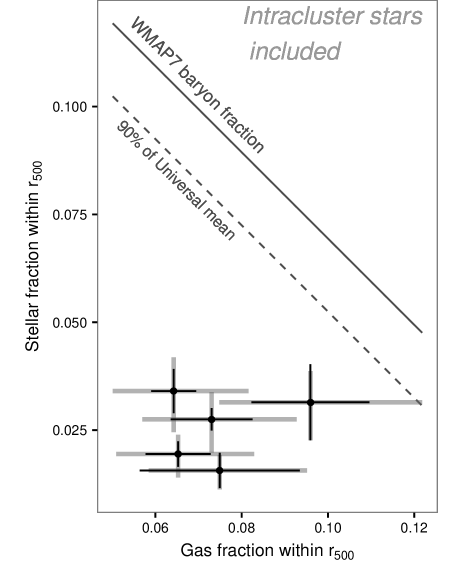
Figure 14: The location of the five clusters in the $f_{\mathrm{star}}$-$f_{\mathrm{gas}}$ plane, compared to the Universal mean baryon fraction. The two different types of error bar show the separate contributions from 1$\sigma$ measurement (thin black) and conservative systematic (thick grey) uncertainties (see Table 6).

5.7 Feedback and missing baryons

There is considerable variation in $f_{\mathrm{b}}$ for these five clusters, which results mainly from the scatter in $f_{\mathrm{gas}}$ (Fig. 8, right panel), as the dominant baryonic component. While there are no indications of a systematic variation of $f_{\mathrm{b}}$ with total mass (Fig. 9), the baryon fractions of these five clusters are lower than those of Gonzalez et al. (in preparation), which are generally more massive. Moreover, in the case of the 3 clusters where we can directly measure both gas and stars out to $r_{\mathrm{500}}$, there is evidently substantial baryon loss. However, it is not clear if this points to a trend with mass, or is the result of a break in self-similarity, as seen to occur at $kT\approx 3.5$ keV (corresponding to $\sim 2.6\times 10^{14}M_{\mathrm{\odot}}$) in a recent analysis of the X-ray luminosity-temperature relation (Maughan et al., 2012).

It is well established that cosmological simulations without radiative cooling or galaxy feedback produce clusters that have baryon fractions within $r_{\mathrm{500}}$ that are consistent with the ‘depleted cosmic’ $f_{\mathrm{b}}$ level of $\sim$0.9 (e.g. Ettori et al., 2006). The introduction of cooling allows baryons to transfer from the hot to the cold phase to form stars and leads to a systematic variation in gas fraction with halo mass (e.g. Muanwong et al., 2001). Indeed, Bode et al. (2009) point out that if stellar fraction varies as steeply as $M_{\mathrm{500}}$^-0.49, then cooling alone can explain the trend of gas fraction with halo mass. However, radiative cooling produces no net loss of baryons– this is clearly inconsistent with our results, which also include the contribution from intracluster stars. Furthermore, the Bode et al. model assumes that the stars have the same radial distribution as the dark matter, whereas our results and those of GZZ07 favour a less extended light distribution than that of the dark matter.

One possible explanation for the missing baryons is therefore galaxy feedback, for which the phenomenon of AGN outflows is the most likely candidate (e.g. Short & Thomas, 2009; McCarthy et al., 2010, 2011), whether prior to or after gravitational collapse. Indeed, it is now known that the feedback associated with galaxy formation and black hole growth is capable of altering the distribution of both baryonic and dark matter even on large scales, thereby rendering cosmological inference sensitive to this localized baryonic physics (Lueker et al., 2010; van Daalen et al., 2011). It is therefore of great importance to understand how cosmic feedback operates, and the corresponding balance of hot and cold baryons in groups and clusters of galaxies. Under this scenario, a diversity in feedback histories amongst the clusters could also account for the scatter in $f_{\mathrm{gas}}$, which dominates the variation in the total baryon content.

Furthermore, the phenomenon of power-law-like $\rho_{\mathrm{gas}}$$(r)$ in the outskirts of groups compared to a steepening in clusters is also seen in recent cosmological simulations where feedback has been incorporated and found able and necessary to produce galaxy groups that match many of the characteristics of observed systems (McCarthy et al., 2010). For example, the shape of the median (group-dominated) gas entropy profile in figure 1 of McCarthy et al. (2010) roughly comprises a steeper inner power law ($<0.2r_{\mathrm{500}}$), turning over to a flatter slope until $\sim$0.9 $r_{\mathrm{500}}$, before steepening again. This behaviour is a consequence of the increased impact of galaxy feedback in the shallower potential wells of groups compared to clusters which, firstly, displaces gas from inner to outer regions and, secondly, lowers the ICM pressure and therefore causes more gas accretion from outside the group (I. McCarthy, private communication). The net effect is a flattening of $\rho_{\mathrm{gas}}$$(r)$ around $r_{\mathrm{500}}$ in groups compared to clusters.

6 Conclusions

We have analysed the hot gas and stellar baryon content of five low-mass galaxy clusters drawn from the optically-selected sample of GZZ07, which includes both a direct mapping of the intracluster light (ICL) as well as the galaxies’ contribution, fully corrected for the effects of projection. We use hydrostatic X-ray cluster modelling of XMM-Newton observations to measure the gas total mass of these objects and the corresponding overdensity radii within which to perform an inventory of baryons ($r_{\mathrm{2500}}$ and $r_{\mathrm{500}}$). We summarize our main findings as follows.

1. For all five clusters our hydrostatic X-ray masses are well in excess of those originally estimated by GZZ07 on the basis of their galaxy velocity dispersions ($\sigma$) and an assumed $\sigma-M_{\mathrm{500}}$ relation, by a factor of between 1.7 and 5.7 times. We also calculate alternative estimates of these X-ray masses using the $M-T_{\mathrm{X}}$ relation of Vikhlinin et al. (2006), and consider a range of possible explanations for this discrepancy (Sections 5.1 & 5.3).

2. We study the stellar fraction vs. $M_{\mathrm{500}}$, compared to the other clusters with similar ICL mapping in GZZ07 and find that, despite the large change in total mass, the 5 clusters largely shift along the trend (since the higher mass implies larger $r_{\mathrm{500}}$, within which $f_{\mathrm{star}}$ is measured).

3. Within $r_{\mathrm{500}}$, we find weighted mean stellar (including ICL), gas and total baryon mass fractions of $0.026\pm 0.003$, $0.070\pm 0.005$ and $0.096\pm 0.006$, respectively, at a corresponding weighted mean $M_{\mathrm{500}}$ of ($1.08_{-0.18}^{+0.21})\times 10^{14}$ M_⊙ (see Table 5). This baryon fraction amounts to 57 per cent of the Universal mean, and implies a deficit of at least $\sim$30 per cent compared to the ‘depleted cosmic’ $f_{\mathrm{b}}$ level of $\sim$0.9$\times\Omega_{b}/\Omega_{m}$ expected in the absence of cooling and feedback (e.g. Ettori et al., 2006). We consider the main sources of systematic error affecting our results and conclude that these are not sufficient to explain the observed shortfall in baryons in 4 of the 5 clusters.

4. In the three cases where we can trace the X-ray emission out to $r_{\mathrm{500}}$, we find no evidence for steepening of the gas density profile, as commonly seen in more massive clusters. This behaviour in consistent with the increased effect of galaxy feedback in shallower potential wells seen in the OWLS cosmological simulations, which leads to gas accumulation around $r_{\mathrm{500}}$ (see Section 5.7). This may also account for the baryon deficit observed within $r_{\mathrm{500}}$, and suggests that the missing baryons are located beyond this radius.

As a result of the upward revision in mass, these systems are now no longer located as far towards the extreme low-mass end of the trend as previously thought (GZZ07), at a scale where the impact of cooling and feedback are most pronounced. Indeed, combined ICL photometry and X-ray mapping of many more low mass groups is clearly needed, to constrain the baryon balance in this important regime. However, this remains observationally challenging, owing to the tension between the need for proximity ($z\ll 0.1$) in X-ray detection of faint group emission vs. the requirement of more compact angular size to provide stable and well-characterized backgrounds for diffuse optical light mapping, which is better achieved nearer $z\sim 0.1$. Given the uncertainly in modelling the gas density profile in the outskirts of groups and low-mass clusters, it is also very important to secure deep X-ray observations that can reach beyond $r_{\mathrm{500}}$ at high signal-to-noise ratio, to avoid extrapolation bias and thereby measure the hot gas mass directly. This would have the added benefit of probing a mass scale and spatial regions which are sensitive to cosmic feedback, and may help uncover at least some of the missing baryons.

References

- Akritas & Bershady (1996) Akritas, M. G., & Bershady, M. A. 1996, ApJ, 470, 706
- Arnaud et al. (2007) Arnaud, M., Pointecouteau, E., & Pratt, G. W. 2007, A&A, 474, L37
- Ascasibar & Diego (2008) Ascasibar, Y., & Diego, J. M. 2008, MNRAS, 383, 369
- Balogh et al. (2011) Balogh, M. L., Mazzotta, P., Bower, R. G., et al. 2011, MNRAS, 412, 947
- Balogh et al. (2008) Balogh, M. L., McCarthy, I. G., Bower, R. G., & Eke, V. R. 2008, MNRAS, 385, 1003
- Beers et al. (1990) Beers, T. C., Flynn, K., & Gebhardt, K. 1990, AJ, 100, 32
- Biviano et al. (2006) Biviano, A., Murante, G., Borgani, S., et al. 2006, A&A, 456, 23
- Bode et al. (2009) Bode, P., Ostriker, J. P., & Vikhlinin, A. 2009, ApJ, 700, 989
- Bower et al. (1997) Bower, R. G., Castander, F. J., Ellis, R. S., Couch, W. J., & Boehringer, H. 1997, MNRAS, 291, 353
- Connelly et al. (2012) Connelly, J. L., Wilman, D. J., Finoguenov, A., et al. 2012, ApJ, 756, 139
- Croston et al. (2008) Croston, J. H., Pratt, G. W., Böhringer, H., et al. 2008, A&A, 487, 431
- Dai et al. (2010) Dai, X., Bregman, J. N., Kochanek, C. S., & Rasia, E. 2010, ApJ, 719, 119
- David et al. (1995) David, L. P., Jones, C., & Forman, W. 1995, ApJ, 445, 578
- Eckert et al. (2012) Eckert, D., Vazza, F., Ettori, S., et al. 2012, A&A, 541, A57
- Ettori & Balestra (2009) Ettori, S., & Balestra, I. 2009, A&A, 496, 343
- Ettori et al. (2006) Ettori, S., Dolag, K., Borgani, S., & Murante, G. 2006, MNRAS, 365, 1021
- Feldmeier et al. (2002) Feldmeier, J. J., Mihos, J. C., Morrison, H. L., Rodney, S. A., & Harding, P. 2002, ApJ, 575, 779
- Gonzalez et al. (2005) Gonzalez, A. H., Zabludoff, A. I., & Zaritsky, D. 2005, ApJ, 618, 195
- Gonzalez et al. (2007) Gonzalez, A. H., Zaritsky, D., & Zabludoff, A. I. 2007, ApJ, 666, 147
- Grevesse & Sauval (1998) Grevesse, N., & Sauval, A. J. 1998, Space Science Reviews, 85, 161
- Hernquist (1990) Hernquist, L. 1990, ApJ, 356, 359
- Hicks et al. (2008) Hicks, A. K., Ellingson, E., Bautz, M., et al. 2008, ApJ, 680, 1022
- Hou et al. (2009) Hou, A., Parker, L. C., Harris, W. E., & Wilman, D. J. 2009, ApJ, 702, 1199
- Jansen et al. (2001) Jansen, F., Lumb, D., Altieri, B., et al. 2001, A&A, 365, L1
- Jarosik et al. (2011) Jarosik, N., et al. 2011, ApJS, 192, 14
- Kalberla et al. (2005) Kalberla, P. M. W., Burton, W. B., Hartmann, D., et al. 2005, A&A, 440, 775
- Kay et al. (2004) Kay, S. T., Thomas, P. A., Jenkins, A., & Pearce, F. R. 2004, MNRAS, 355, 1091
- Krick & Bernstein (2007) Krick, J. E., & Bernstein, R. A. 2007, AJ, 134, 466
- Lin et al. (2004) Lin, Y., Mohr, J. J., & Stanford, S. A. 2004, ApJ, 610, 745
- Lueker et al. (2010) Lueker, M., et al. 2010, ApJ, 719, 1045
- Maughan et al. (2012) Maughan, B. J., Giles, P. A., Randall, S. W., Jones, C., & Forman, W. R. 2012, MNRAS, 421, 1583
- McCarthy et al. (2011) McCarthy, I. G., Schaye, J., Bower, R. G., et al. 2011, MNRAS, 412, 1965
- McCarthy et al. (2010) McCarthy, I. G., Schaye, J., Ponman, T. J., et al. 2010, MNRAS, 406, 822
- McGee & Balogh (2010) McGee, S. L., & Balogh, M. L. 2010, MNRAS, 403, L79
- McLaughlin (1999) McLaughlin, D. E. 1999, AJ, 117, 2398
- Muanwong et al. (2001) Muanwong, O., Thomas, P. A., Kay, S. T., Pearce, F. R., & Couchman, H. M. P. 2001, ApJ, 552, L27
- Nagai & Lau (2011) Nagai, D., & Lau, E. T. 2011, ApJ, 731, L10
- Nagai et al. (2007) Nagai, D., Vikhlinin, A., & Kravtsov, A. V. 2007, ApJ, 655, 98
- Navarro et al. (1995) Navarro, J. F., Frenk, C. S., & White, S. D. M. 1995, MNRAS, 275, 720
- Osmond & Ponman (2004) Osmond, J. P. F., & Ponman, T. J. 2004, MNRAS, 350, 1511
- Piffaretti & Valdarnini (2008) Piffaretti, R., & Valdarnini, R. 2008, A&A, 491, 71
- Rasia et al. (2006) Rasia, E., Ettori, S., Moscardini, L., et al. 2006, MNRAS, 369, 2013
- Rasmussen & Ponman (2004) Rasmussen, J., & Ponman, T. J. 2004, MNRAS, 349, 722
- Rasmussen et al. (2006) Rasmussen, J., Ponman, T. J., Mulchaey, J. S., Miles, T. A., & Raychaudhury, S. 2006, MNRAS, 373, 653
- Rykoff et al. (2008a) Rykoff, E. S., McKay, T. A., Becker, M. R., et al. 2008a, ApJ, 675, 1106
- Rykoff et al. (2008b) Rykoff, E. S., Evrard, A. E., McKay, T. A., et al. 2008b, MNRAS, 387, L28
- Sanderson et al. (2009a) Sanderson, A. J. R., Edge, A. C., & Smith, G. P. 2009a, MNRAS, 398, 1698
- Sanderson et al. (2009b) Sanderson, A. J. R., O’Sullivan, E., & Ponman, T. J. 2009b, MNRAS, 395, 764
- Sanderson & Ponman (2010) Sanderson, A. J. R., & Ponman, T. J. 2010, MNRAS, 402, 65
- Sanderson et al. (2003) Sanderson, A. J. R., Ponman, T. J., Finoguenov, A., Lloyd-Davies, E. J., & Markevitch, M. 2003, MNRAS, 340, 989
- Sanderson et al. (2006) Sanderson, A. J. R., Ponman, T. J., & O’Sullivan, E. 2006, MNRAS, 372, 1496
- Short & Thomas (2009) Short, C. J., & Thomas, P. A. 2009, ApJ, 704, 915
- Sivanandam et al. (2009) Sivanandam, S., Zabludoff, A. I., Zaritsky, D., Gonzalez, A. H., & Kelson, D. D. 2009, ApJ, 691, 1787
- Skrutskie et al. (2006) Skrutskie, M. F., et al. 2006, AJ, 131, 1163
- Snowden et al. (2004) Snowden, S. L., Collier, M. R., & Kuntz, K. D. 2004, ApJ, 610, 1182
- Sun et al. (2009) Sun, M., Voit, G. M., Donahue, M., et al. 2009, ApJ, 693, 1142
- Thode (2002) Thode, H. C. 2002, Testing for Normality (CRC Press)
- Urban et al. (2011) Urban, O., Werner, N., Simionescu, A., Allen, S. W., & Böhringer, H. 2011, MNRAS, 414, 2101
- van Daalen et al. (2011) van Daalen, M. P., Schaye, J., Booth, C. M., & Dalla Vecchia, C. 2011, MNRAS, 415, 3649
- Venables & Ripley (2002) Venables, W. N., & Ripley, B. D. 2002, Modern Applied Statistics with S, 4th edn. (New York: Springer), iSBN 0-387-95457-0
- Vikhlinin et al. (2007) Vikhlinin, A., Burenin, R., Forman, W. R., et al. 2007, in Heating versus Cooling in Galaxies and Clusters of Galaxies, ed. H. Böhringer, G. W. Pratt, A. Finoguenov, & P. Schuecker, 48
- Vikhlinin et al. (1999) Vikhlinin, A., Forman, W., & Jones, C. 1999, ApJ, 525, 47
- Vikhlinin et al. (2006) Vikhlinin, A., Kravtsov, A., Forman, W., et al. 2006, ApJ, 640, 691
- Voit & Bryan (2001) Voit, G. M., & Bryan, G. L. 2001, Nature, 414, 425
- Wickham (2009) Wickham, H. 2009, ggplot2: elegant graphics for data analysis (Springer New York), iSBN 978-0-387-98140-6
- Zaritsky et al. (2006) Zaritsky, D., Gonzalez, A. H., & Zabludoff, A. I. 2006, ApJ, 638, 725
- Zibetti et al. (2005) Zibetti, S., White, S. D. M., Schneider, D. P., & Brinkmann, J. 2005, MNRAS, 358, 949