Soft local times and decoupling of random interlacements

Abstract

In this paper we establish a decoupling feature of the random interlacement process $\mathcal{I}^{u}\subset\mathbb{Z}^{d}$ at level $u$, $d\geq 3$. Roughly speaking, we show that observations of $\mathcal{I}^{u}$ restricted to two disjoint subsets $A_{1}$ and $A_{2}$ of $\mathbb{Z}^{d}$ are approximately independent, once we add a sprinkling to the process $\mathcal{I}^{u}$ by slightly increasing the parameter $u$. Our results differ from previous ones in that we allow the mutual distance between the sets $A_{1}$ and $A_{2}$ to be much smaller than their diameters. We then provide an important application of this decoupling for which such flexibility is crucial. More precisely, we prove that, above a certain critical threshold $u_{**}$, the probability of having long paths that avoid $\mathcal{I}^{u}$ is exponentially small, with logarithmic corrections for $d=3$.

To obtain the above decoupling, we first develop a general method for comparing the trace left by two Markov chains on the same state space. This method is based in what we call the soft local time of a chain. In another crucial step towards our main result, we also prove that any discrete set can be “smoothened” into a slightly enlarged discrete set, for which its equilibrium measure behaves in a regular way. Both these auxiliary results are interesting in themselves and are presented independently from the rest of the paper.

Keywords. Random interlacements, stochastic domination, soft local time, connectivity decay, smoothening of discrete sets.

1 Introduction and results

This work is mainly concerned with the decoupling of the random interlacements model introduced by A.S. Sznitman in [23]. In other words, we show that the restrictions of the interlacement set $\mathcal{I}^{u}$ to two disjoint subsets $A_{1}$ and $A_{2}$ of $\mathbb{Z}^{d}$ are approximately independent in a certain sense. To this aim, we first develop a general method, based on what we call soft local times, to obtain an approximate stochastic domination between the ranges of two general Markov chains on the same state space.

To apply this coupling method to the model of random interlacements, we first need to modify the sets $A_{1}$ and $A_{2}$ through a procedure we call smoothening. This consists of enclosing a discrete set $A\subset\mathbb{Z}^{d}$ into a slightly enlarged set $A^{\prime}$, whose equilibrium distribution behaves “regularly”, resembling what happens for a large discrete ball.

Finally, as an application of our decoupling result, we obtain upper bounds for the connectivity function of the vacant set $\mathcal{V}^{u}=\mathbb{Z}^{d}\setminus\mathcal{I}^{u}$, for intensities $u$ above a critical threshold $u_{**}$. These bounds are considerably sharp, presenting a behavior very similar to that of their corresponding lower bounds.

We believe that these four results are interesting in their own. Therefore, we structured the article in a way so they can be read independently from each other. Below we give a more detailed description of each of these results.

1.1 Decoupling of random interlacements

The primary interest of this work lies in the study of the random interlacements process, recently introduced by A.-S. Sznitman in [23]. The construction of random interlacements was originally motivated by the analysis of the trace left by simple random walk on large graphs, for instance a large discrete torus or a thick discrete cylinder. Intuitively speaking, this model describes the texture in the bulk left by these trajectories, when the random walk is let run up to specific time scales.

Recently, a great effort has been spent in the study of this model [18], [19], [31], [24], [25], [14], and [4] as well as in establishing rigorously the relation between random interlacements and the trace left by random walks on large graphs, see [20], [34], [32] and [3]. Recent works have also shown a connection between: random interlacements, the Gaussian free field [28], [27] and cover times of random walks [2].

Roughly speaking, the model of random interlacements can be described as an Poissonian cloud of doubly infinite random walk trajectories on $\mathbb{Z}^{d}$, $d\geq 3$. The density of this cloud is governed by an intensity parameter $u>0$ so that, as $u$ increases, more and more trajectories enter the picture. We denote by $\mathcal{I}^{u}$ the so called interlacement set, given by the union of the range of these random walk trajectories. Regarding $\mathcal{I}^{u}$ as a random subset of $\mathbb{Z}^{d}$, its law $\mathcal{Q}^{u}$ can be characterized as the only distribution in $\{0,1\}^{\mathbb{Z}^{d}}$ such that

$$\mathcal{Q}^{u}[K\cap\mathcal{I}^{u}=\varnothing]=\exp\{-u\operatorname{cap}(K)\},\text{ for every finite $K\subset\mathbb{Z}^{d}$},$$ (1.1)

where $\operatorname{cap}(K)$ stands for the capacity of the set $K$ defined in (2.6), see Proposition 1.5 of [23] for the characterization (1.1).

The main difficulty in understanding properties of $\mathcal{I}^{u}$ is related to its long range dependence. Let us note for instance that

$$\operatorname{Cov}({{1}}_{x\in\mathcal{I}^{u}},{{1}}_{y\in\mathcal{I}^{u}})\sim\frac{c_{d}u}{\|x-y\|^{d-2}}\quad\text{ as }\quad\|x-y\|\to\infty,$$ (1.2)

see [23], (1.68). Such a slow decay of correlations imposes several obstacles to the analysis of random interlacements, especially in low dimensions. Various methods have been developed in order to circumvent this dependence, some of which we briefly summarize below.

Let us explain what is the type of statement we are after. Consider two subsets $A_{1}$ and $A_{2}$ of $\mathbb{Z}^{d}$ with diameters smaller or equal to $r$ and within distance at least $s\geq 1$ from each other. Suppose also that we are given two functions $f_{1}:\{0,1\}^{A_{1}}\to[0,1]$ and $f_{2}:\{0,1\}^{A_{2}}\to[0,1]$ that depend only on the configuration of the random interlacements inside the sets $A_{1}$ and $A_{2}$ respectively. In [23], (2.15) it was established that

$$\operatorname{Cov}(f_{1},f_{2})\leq c_{d}u\frac{\operatorname{cap}(A_{1})\operatorname{cap}(A_{2})}{s^{d-2}}\leq c^{\prime}_{d}u\Big{(}\frac{r^{2}}{s}\Big{)}^{d-2},$$ (1.3)

see also Lemma 2.1 of [1]. Although the above inequality retains the slow polynomial decay observed in (1.2), it has been useful in various situations, see for instance Theorem 4.3 of [23] and Theorem 0.1 of [1].

A first improvement on (1.3) appeared already in the pioneer work [23], where the author considers what he calls ‘sprinkling’ of the law $\mathcal{I}^{u}$, see Section 3. In the sprinkling procedure, “independent paths are thrown in, so as to dominate long range dependence” of $\mathcal{I}^{u}$.

Given two functions $f_{1}$ and $f_{2}$ as above, which are non-increasing in $\mathcal{I}^{u}$, the technique of Section 3 of [23] allows one to conclude that, roughly speaking,

$$\mathcal{Q}^{u}[f_{1}f_{2}]\leq\mathcal{Q}^{u(1+\delta)}[f_{1}]\mathcal{Q}^{u(1+\delta)}[f_{2}]+c_{d,\alpha}\Big{(}\frac{r}{s}\Big{)}^{\alpha},$$ (1.4)

where $\alpha$ is arbitrary and the sprinkling parameter $\delta$ goes to zero as a polynomial of $(r/s)$. Note that the above represents a big improvement over (1.3): in exchange to restricting ourselves to non-increasing functions and introducing a sprinkling term, we obtain a much faster decay in the error term. Since its introduction, the sprinkling technique has been useful for several problems on random interlacements, see [21], [26], and [32].

The most recent result on decoupling bounds for interlacements can be found in [26] and stands out for several reasons. First, it generalizes the ideas behind [19] and [31] for random interlacements on quite general classes of graphs (besides $\mathbb{Z}^{d}$), as long as they satisfy certain heat kernel estimates. Secondly, the tools developed in [26] work both to show existence and absence of percolation through a unified framework and give novel results even in the particular case of $\mathbb{Z}^{d}$, see also the beautiful applications in [15] and [6].

On the other hand, the results in [26] were designed having a renormalization scheme in mind. Thus, their use is restricted to bounding the so-called ‘cascading events’, which behave in a certain hierarchical way, see the details in Section 3 of [26].

Although the results in (1.3), (1.4) and [26] complement each other, they suffer from the same drawback, as they implicitly assume that

the distance between $$A_{1} A_{2}$$ and is at least of the same order as their diameters. (1.5)

This can be a major obstruction in some applications, such as the one we present in Section 3 on the decay of connectivity.

Let us now state the main theorem of the present paper, which can be regarded as an improvement on (1.4). Later we will describe precisely how it differs quantitatively from previously known results.

Below, $\gamma_{\textnormal{\tiny\ref{c:main'}}}$ and $\gamma_{\textnormal{\tiny\ref{c:main''}}}$ are positive constants depending only on the dimension $d$.

Theorem 1.1.

Let $A_{1},A_{2}$ be two non intersecting subsets of $\mathbb{Z}^{d}$, with at least one of them being finite. Let $s$ be the distance between $A_{1}$ and $A_{2}$, and $r$ be the minimum of their diameters. Then, for all $u>0$ and $\varepsilon\in(0,1)$ we have

• for any increasing functions $f_{1}:\{0,1\}^{A_{1}}\to[0,1]$ and $f_{2}:\{0,1\}^{A_{2}}\to[0,1]$,

  $$\mathcal{Q}^{u}[f_{1}f_{2}]\leq\mathcal{Q}^{(1+\varepsilon)u}[f_{1}]\mathcal{Q}^{(1+\varepsilon)u}[f_{2}]+\gamma_{\textnormal{\tiny\ref{c:main'}}}(r+s)^{d}\exp(-\gamma_{\textnormal{\tiny\ref{c:main''}}}\varepsilon^{2}us^{d-2});$$ (1.6)

• for any decreasing functions $f_{1}:\{0,1\}^{A_{1}}\to[0,1]$ and $f_{2}:\{0,1\}^{A_{2}}\to[0,1]$,

  $$\mathcal{Q}^{u}[f_{1}f_{2}]\leq\mathcal{Q}^{(1-\varepsilon)u}[f_{1}]\mathcal{Q}^{(1-\varepsilon)u}[f_{2}]+\gamma_{\textnormal{\tiny\ref{c:main'}}}(r+s)^{d}\exp(-\gamma_{\textnormal{\tiny\ref{c:main''}}}\varepsilon^{2}us^{d-2}).$$ (1.7)

We of course assume the above functions $f_{1}$ and $f_{2}$ to be measurable (recall that one of the sets $A_{1}$ or $A_{2}$ may be infinite).

The above theorem is a direct consequence of the slightly more general Theorem 2.1. Note that the opposite inequalities to (1.6) and (1.7) follow without error terms (and with $\varepsilon=0$) by the FKG inequality, which was proved for random interlacements in [29], Theorem 3.1.

Let us now stress what are the main improvements offered by the above bounds over previously known results. First, there is no requirement that $s$ should be larger than $r$ as in (1.5) (and again, one of the sets may even be infinite). Moreover, these error bounds feature an explicit and fast decay on $s$, even as $\varepsilon=\varepsilon(s,r)$ goes (not too rapidly) to zero. We include in Remark 3.3 some observations on how close to optimal one can expect (1.6) and (1.7) to be.

1.2 Connectivity decay

As an application of Theorem 1.1, we establish a result on the decay of connectivity on the vacant set $\mathcal{V}^{u}=\mathbb{Z}^{d}\setminus\mathcal{I}^{u}$. More precisely, for $u$ large enough (see Theorem 3.1 for details), for $d\geq 4$,

$$\mathcal{Q}^{u}[0\xleftrightarrow{\mathcal{V}^{u}}x]\leq\gamma_{\textnormal{\tiny\ref{c:connect}}}\exp\{-\gamma_{\textnormal{\tiny\ref{c:connect2}}}\|x\|\},\text{ for every $x\in\mathbb{Z}^{d}$.}$$ (1.8)

where $\gamma_{\textnormal{\tiny\ref{c:connect}}}$ and $\gamma_{\textnormal{\tiny\ref{c:connect2}}}$ depend only on $d$. If $d=3$ and $u$ is large enough, then for any $b>1$ there exist $\gamma_{\textnormal{\tiny\ref{c:connect_dim3}}}=\gamma_{\textnormal{\tiny\ref{c:connect_dim3}}}(u,b)$ and $\gamma_{\textnormal{\tiny\ref{c:connect2_dim3}}}=\gamma_{\textnormal{\tiny\ref{c:connect2_dim3}}}(u,b)$ such that

$$\mathcal{Q}^{u}[0\xleftrightarrow{\mathcal{V}^{u}}x]\leq\gamma_{\textnormal{\tiny\ref{c:connect_dim3}}}\exp\Big{\{}-\gamma_{\textnormal{\tiny\ref{c:connect2_dim3}}}\frac{\|x\|}{\log^{3b}\|x\|}\Big{\}},\text{ for every $x\in\mathbb{Z}^{3}$.}$$ (1.9)

see Theorem 3.1 and Remark 3.2 for more details.

Let us stress that the above bounds greatly improve on the previously known results, proved in Theorem 0.1 of [19]. There, the authors establish similar bounds but with $\|x\|$ replaced by $\|x\|^{\rho}$ for some unknown exponent $\rho\in(0,1)$. Our bounds on the other hand are considerably sharp, as they closely resemble the corresponding lower bounds, see Remark 3.2 for details.

Note that the exponential decay in (1.8) is also observed in independent percolation models, see for instance Theorem (5.4) of [8], p.88 and [11]. However, due to the strong dependence present in $\mathcal{V}^{u}$, its validity was at first not obvious to the authors. For one reason, it is known that the logarithmic factor in (1.9) cannot be dropped, see Remark 3.2 below. Similar types of non exponential decays in dependent percolation models can be found for instance in (1.65) and (2.21) of [23] and Remark 3.7 2) of [31].

Finally we would like to stress that our proof of (1.8)–(1.9) is general enough in the sense that it could be adapted for other dependent percolation models, as long as they satisfy a suitable decoupling inequality. See the discussion in Remark 3.4.

1.3 Soft local times

In Section 4 we develop a technique to prove approximate stochastic domination of the trace left by a Markov chain on a metric space. This is an important ingredient in proving Theorem 1.1 and we also expect it to be useful in future applications. To illustrate this technique, consider an irreducible Markov chain $(Z_{i})_{i\geq 1}$ on a finite state space $\Sigma$ having $\pi$ as its unique stationary measure.

A typical model to keep in mind is a random walk on a torus that jumps from $z$ to a uniformly chosen point in the ball centered in $z$ with radius $k$. By transitiveness, the uniform distribution $\pi$ is clearly invariant. Intuitively speaking, if we let this Markov chain run for a long time $t$, we expect the law of covered set $\{Z_{1},\dots,Z_{t}\}$ to be “reasonably close” to that of a collection $\{W_{1},\dots,W_{t}\}$ of i.i.d. points in $\Sigma$ distributed according to $\pi$. This is made precise in the following result, which is a consequence of Corollary 4.4.

Proposition 1.2.

Let $(Z_{i})_{i\geq 1}$ be a Markov chain on a finite set $\Sigma$, with transition probabilities $p(z,z^{\prime})$, initial distribution $\pi_{0}$, and stationary measure $\pi$. Then we can find a coupling $\mathbb{Q}$ between $(Z_{i})$ and an i.i.d. collection $(W_{i})$ (with law $\pi$), in such a way that for any $\lambda>0$ and $t\geq 0$,

$$\begin{split}\mathbb{Q}\big{[}\{Z_{1},\dots,Z_{t}\}&\subset\{W_{1},\dots,W_{R}\}\big{]}\\ &\geq\mathbb{Q}\Big{[}\xi_{0}\pi_{0}(z)+\sum_{j=1}^{t-1}\xi_{j}p(Z_{j},z)\leq\lambda\pi(z),\text{ for all $z\in\Sigma$}\Big{]},\end{split}$$ (1.10)

where $\xi_{i}$ are i.i.d. $\mathrm{Exp}(1)$ random variables, independent of $R$, a $\mathrm{Poisson}(\lambda)$-distributed random variable.

Observe that the above statement can have interesting consequences in bounding the hitting time of a given subset of $\Sigma$, see (2.4) for a precise definition.

We call the sum $\sum_{j}\xi_{j}p(Z_{j},z)$ the soft local time of the chain $Z_{j}$. To justify this notation, observe that instead of counting the number of visits to a fixed site (which corresponds to the usual notion of local time), we are summing up the chances of visiting such site, multiplied by i.i.d. mean-one positive factors. See also Theorem 4.6.

In Remark 4.5 we describe the main advantages of Proposition 1.2 over previous domination techniques and how it allows us to drop the assumption (1.5).

Later in Section 4, we establish general estimates on the expectation, variance and exponential moments of the soft local time $\sum_{j}\xi_{j}p(Z_{j},z)$. These are based on regularity assumptions on the transition probabilities $p(\cdot,\cdot)$ and are valuable when estimating the right hand side of (1.10) by means of exponential Chebyshev’s inequalities, see Theorems 4.6, 4.8 and 4.9.

Now, we comment on the main method employed to prove results such as Proposition 1.2 above. One can better visualize the picture in a continuous space, so we use another example to illustrate the method: assume that we are given a sequence of (not necessarily independent nor Markovian) random variables $S_{1},S_{2},S_{3},\ldots$ taking values in the interval $[0,1]$, and let $T$ be a finite stopping time. As in (1.10), we attempt to dominate this process by a sequence $U_{1},\ldots,U_{N}$, where $(U_{k})$ are i.i.d. Uniform$[0,1]$ random variables, and $N$ is a Poisson random variable independent of $(U_{k})$. More precisely, we want to construct a coupling between the two sequences in such a way that

$$\{S_{1},\ldots,S_{T}\}\subseteq\{U_{1},\ldots,U_{N}\}$$ (1.11)

with probability close to one. We assume that the law of $S_{k}$ conditioned on $S_{1},\ldots,S_{k-1}$ is absolutely continuous with respect to the Lebesgue measure on $[0,1]$, see (4.6).

Our method for obtaining such a coupling is illustrated on Figure 1. Consider a Poisson point process in $[0,1]\times\mathbb{R}_{+}$ with rate $1$. Then, one can obtain a realization of the $U$-sequence by simply retaining the first coordinate of the points lying below a given threshold (the dashed line in Figure 1) corresponding to the parameter of the Poisson random variable $N$.

Now, in order to obtain a realization of the $S$-sequence using the same Poisson point process, one proceeds as follows:

• first, take the density $g(\cdot)$ of $S_{1}$ and multiply it by the unique positive number $\xi_{1}$ so that there is exactly one point of the Poisson process lying on the graph of $\xi_{1}g$ and nothing strictly below it;

• then consider the conditional density $g(\cdot\mid S_{1})$ of $S_{2}$ given $S_{1}$ and find the smallest constant $\xi_{2}$ so that exactly two points lie underneath $\xi_{2}g(\cdot\mid S_{1})+\xi_{1}g(\cdot)$;

• continue with $g(\cdot\mid S_{1},S_{2})$, and so on, up to time $T$, as shown on Figure 1.

In Proposition 4.3, we show that the collection of points obtained through the above procedure has the same law as $(S_{1},S_{2},\dots)$ and is independent of the random variables $\xi_{i}$, which are i.i.d. with law Exp($1$). We call the sum $\xi_{1}g(\cdot)+\xi_{2}g(\cdot\mid S_{1})+\cdots$ the soft local time of the process $S$ (which coincides with the sum in the right-hand side of (1.10) in the Markovian case). Clearly, if the soft local time (the gray area on the picture) is below the dashed line, then the domination in (1.11) holds. To obtain the probability of a successful coupling, one has to estimate the probability that the soft local time lies below the dashed line. In several cases, this reduces to a large deviations estimate.

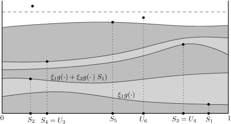
Figure 1: Soft local times: the construction of the process $S$ (here, $T=5$, $N=6$, $U_{k}=S_{k}$ for $k=1,2,5$); it is very important to observe that the points of the two processes need not necessarily appear in the same order with respect to the vertical axis, see Remark 4.5.

After developing a general version of this technique in Section 4, we adapt this theory to random interlacements in Section 5. More precisely, we present an alternative construction of the interlacement set $\mathcal{I}^{u}$ restricted to some $A\subset\mathbb{Z}^{d}$. In this construction, we split each trajectory composing $\mathcal{I}^{u}$ into a collection of excursions in and out of $A$. This induces a Markov chain on the space of excursions and the techniques of soft local times helps us control the range of such soup.

After the conclusion of this article, we learned that a technique similar to the soft-local times was introduced in the special case $\Sigma=(0,1)\subset\mathbb{R}$ in order to study local minima of the Brownian motion. see Claim 1.5 of [33].

We believe that the method of soft local time can be useful in other contexts besides random interlacements. For example, when considering a random walk trajectory on a finite graph (such as a torus or a discrete cylinder), one can naturally be interested in the degree of independence in the pictures left by the walker on disjoint subsets of the graph. The approach followed in this paper is likely to be successful in this situation as well. We also believe this technique could give alternative proofs or generalize results on the coupling of systems of independently moving particles, see Proposition 5.1 of [13] for an example of such a statement.

1.4 Smoothening of discrete sets

As we mentioned before, in order to estimate the probability of having a successful coupling using the soft local times technique, we need some regularity conditions on the transition densities of the Markov chain. When applying this to the excursions composing the random interlacements, this translates into a condition on the regularity of the entrance distributions on the sets $A_{1}$ and $A_{2}$, which may not hold in general (picture for instance a set with sharp points).

To overcome this difficulty, we develop a technique to enlarge the original discrete sets $A_{1}$ and $A_{2}$ into slightly bigger discrete sets with “sufficiently smooth” boundaries, so that their entrance probabilities satisfy the required regularity conditions.

The exact result we are referring to is given in Proposition 6.1, but we provide here a small preview of its statement. There exist positive constants $c,c^{\prime},c^{\prime\prime},s_{0}$ (depending only on dimension) such that for any $s\geq s_{0}$ and any finite set $A\subset\mathbb{Z}^{d}$, there exist a set $A^{(s)}$ with $A\subseteq A^{(s)}\subseteq B(A,s)$ and

$$P_{x}[X_{H}=y]\leq cP_{x}[X_{H}=y^{\prime}],$$ (1.12)

for all $y,y^{\prime}\in\partial A^{(s)}$ with $\|y-y^{\prime}\|\leq c^{\prime\prime}s$, and all $x$ such that $\|x-y\|\geq c^{\prime}s$. Where $X$ is the simple random walk and $H$ is the hitting time of the set $A^{(s)}$. That is, the entrance measure to the set $A^{(s)}$ is “comparable” in close sites of the boundary, as long as the starting point of the random walk is sufficiently far away.

It is important to observe that for example a large (discrete) ball fulfills the above property, while a large box does not, since its entrance probabilities at the faces are typically much smaller than those at the corners (to see this, observe that one can obtain using the arguments similar e.g. to the proof of Theorem 1.4 of [12] that the harmonic measure at a corner of the box is at least $O(n^{-\gamma})$ for some $\gamma<1$, while for “generic” sites on the faces it is $O(n^{-1})$).

1.5 Plan of the paper

The paper is organized in the following way. In Section 2 we formally define the model of random interlacements, and state our main decoupling result. In Section 3, we state the connectivity decay stated in (1.7) and (1.6), see Theorem 3.1. In Section 4 we present a general version of the method of soft local times. Then, in Section 5 this method is used to introduce an alternative construction of random interlacements, which is better suited for decoupling configurations on disjoint sets. In the same section we reduce the proof of our main Theorem 2.1 to a large deviations estimate for the soft local time of excursions. In Section 6, we estimate the probability of these large deviation events and conclude the proof of Theorem 2.1 under a set of additional assumptions on the entrance measures of $A_{1,2}$. While this set of assumptions may not be satisfied for arbitrary $A_{1,2}$, we show in Section 8 that this is not really an issue, as one can always enlarge slightly the sets of interest (with the procedure referred above as smoothening) so that these modified sets satisfy the necessary regularity assumptions. Before going to (quite technical) Section 8, in Section 7 we prove the result on the decay of connectivity for the vacant set, corresponding to (1.8) and (1.9).

2 Random interlacements: formal definitions and main result

In this paper, we use the following convention concerning constants: $c_{1},c_{2},c_{3},\ldots$, as well as $\gamma_{1},\gamma_{2},\gamma_{3},\ldots$ denote strictly positive constants depending only on dimension $d$. Dependence of constants on additional parameters appears in the notation. For example, $c_{\alpha}$ denotes a constant depending only on $d$ and $\alpha$. Also $c$-constants are “local” (used only in a small neighborhood of the place of the first appearance) while $\gamma$-constants are “nonlocal” (they appear in propositions and “important” formulas).

Let us now introduce some notation and describe the model of random interlacements. In addition, we recall some useful facts concerning the model.

For $a\in\mathbb{R}$, we write $\lfloor a\rfloor$ for the largest integer smaller or equal to $a$ and recall that

$$\lfloor ta+(1-t)b\rfloor\in[\min\{a,b\},\max\{a,b\}],\text{ for all }a,b\in\mathbb{Z}\text{ and }t\in[0,1].$$ (2.1)

We say that two points $x,y\in\mathbb{Z}^{d}$ are neighbors if they are at Euclidean distance (denoted by $\|\cdot\|$) exactly $1$ (we also write $x\leftrightarrow y$ when $x$ and $y$ are neighbors). This induces a graph structure and a notion of connectedness in $\mathbb{Z}^{d}$.

If $K\subset\mathbb{Z}^{d}$, we denote by $K^{c}$ its complement and by $B(K,r)$ the $r$-neighborhood of $K$ with respect to the Euclidean distance, i.e. the union of the balls $B(x,r)$ for $x\in K$. The diameter of $K$ (denoted by $\operatorname{diam}(K)$) is the supremum of $\|x-y\|_{\infty}$ with $x,y\in K$, where $\|\cdot\|_{\infty}$ is the maximum norm. Let us define its internal boundary $\partial K=\{x\in K;x\leftrightarrow y$ for some $y\in K^{c}\}$.

In this article the term path always denotes finite, nearest neighbor paths, i.e. some $\mathcal{T}:\{0,\dots,n\}\rightarrow\mathbb{Z}^{d}$ such that $\mathcal{T}(l)\leftrightarrow\mathcal{T}(l+1)$ for $l=0,\dots,n-1$. In this case we say that the length of $\mathcal{T}$ is $n$.

Let us denote by $W_{+}$ and $W$ the spaces of infinite, respectively doubly infinite, transient trajectories

$$\begin{split}W_{+}=\Big{\{}w:\mathbb{Z}_{+}\rightarrow\mathbb{Z}^{d};w(l)\leftrightarrow w(l+1),\text{ for each }l\geq 0\text{ and }\|w(l)\|\xrightarrow[l\rightarrow\infty]{}\infty\Big{\}},\\ W=\Big{\{}w:\mathbb{Z}\rightarrow\mathbb{Z}^{d};w(l)\leftrightarrow w(l+1),\text{ for each }l\in\mathbb{Z}\text{ and }\|w(l)\|\xrightarrow[|l|\rightarrow\infty]{}\infty\Big{\}}.\end{split}$$ (2.2)

We endow these spaces with the $\sigma$-algebras $\mathcal{W}_{+}$ and $\mathcal{W}$ generated by the coordinate maps $\{X_{n}\}_{n\in\mathbb{Z}_{+}}$ and $\{X_{n}\}_{n\in\mathbb{Z}}$.

Let us also introduce the entrance time of a finite set $K\subset\mathbb{Z}^{d}$

$$H_{K}(w)=\inf\{k;X_{k}(w)\in K\},\text{ for }w\in W_{(+)},\\$$ (2.3)

and for $w\in W_{+}$, we define the hitting time of $K$ as

$$\widetilde{H}_{K}(w)=\inf\{k\geq 1;X_{k}(w)\in K\}.$$ (2.4)

Let $\theta_{k}:W\rightarrow W$ stand for the time shift given by $\theta(w)(\cdot)=w(\,\cdot+k)$ (where $k$ could also be a random time).

For $x\in\mathbb{Z}^{d}$, (recall that $d\geq 3$) we can define the law $P_{x}$ of a simple random walk starting at $x$ on the space $(W_{+},\mathcal{W}_{+})$. If $\rho$ is a measure on $\mathbb{Z}^{d}$, we write $P_{\rho}=\sum_{x\in\mathbb{Z}^{d}}\rho(x)P_{x}$.

Let us introduce, for a finite $K\subset\mathbb{Z}^{d}$, the equilibrium measure

$$e_{K}(x)={{1}}_{x\in K}P_{x}[\widetilde{H}_{K}=\infty],\text{ for }x\in\mathbb{Z}^{d},$$ (2.5)

the capacity of $K$

$$\text{cap}(K)=e_{K}(\mathbb{Z}^{d})$$ (2.6)

and the normalized equilibrium measure

$$\overline{e}_{K}(x)=e_{K}(x)/\text{cap}(K),\text{ for }x\in\mathbb{Z}^{d}.$$ (2.7)

We mention the following bound on the capacity of a ball of radius $r\geq 1$

$$\operatorname{cap}(B(0,r))\asymp r^{d-2}$$ (2.8)

see Proposition 6.5.2 of [10] (here and in the sequel we write $f(r)\asymp g(r)$ when $c_{\textnormal{\tiny\ref{c:cap}}}g(r)\leq f(r)\leq c_{\textnormal{\tiny\ref{c:cap1}}}g(r)$ for strictly positive constants $c_{\textnormal{\tiny\ref{c:cap}}},c_{\textnormal{\tiny\ref{c:cap1}}}$ depending only on the dimension).

Let $W^{*}$ stand for the space of doubly infinite trajectories in $W$ modulo time shift,

$$W^{*}=W/\sim\mbox{, where }w\sim w^{\prime}\mbox{ if }w(\cdot)=w^{\prime}(k+\cdot),\mbox{ for some }k\in\mathbb{Z},$$ (2.9)

endowed with the $\sigma$-algebra

$$\mathcal{W}^{*}=\{A\subset W^{*};(\pi^{*})^{-1}(A)\in\mathcal{W}\},$$ (2.10)

which is the largest $\sigma$-algebra making the canonical projection $\pi^{*}:W\rightarrow W^{*}$ measurable. For a finite set $K\subset\mathbb{Z}^{d}$, we denote as $W_{K}$ the set of trajectories in $W$ which meet the set $K$ and define $W^{*}_{K}=\pi^{*}(W_{K})$.

Now we are able to describe the intensity measure of the Poisson point process which governs the random interlacements.

For a finite set $K\subset\mathbb{Z}^{d}$, we consider the measure $Q_{K}$ in $(W,\mathcal{W})$ supported in $W_{K}$ such that, given $A,B\in\mathcal{W}_{+}$ and $x\in K$,

$$Q_{K}[(X_{-n})_{n\geq 0}\in A,X_{0}=x,(X_{n})_{n\geq 0}\in B]=P_{x}[A\mid\tilde{H}_{K}=\infty]P_{x}[B]e_{K}(x).$$ (2.11)

Theorem 1.1 of [23] establishes the existence of a unique $\sigma$-finite measure $\nu$ in $W^{*}$ such that,

$$1_{W_{K}^{*}}\cdot\nu=\pi^{*}\circ Q_{K},\text{ for any finite set $K\subset\mathbb{Z}^{d}$.}$$ (2.12)

The above equation is the main tool to perform calculations on random interlacements.

We then introduce the spaces of point measures on $W^{*}\times\mathbb{R}_{+}$ and $W_{+}\times\mathbb{R}_{+}$

$$\begin{split}\Omega&=\bigg{\{}\;\;\omega=\smash{\sum_{i\geq 1}}\delta_{(w^{*}_{i},u_{i})}\Big{|}\;\;\begin{split}&w^{*}_{i}\in W^{*},u_{i}\in\mathbb{R}_{+}\mbox{ and }\omega(W^{*}_{K}\times[0,u])<\infty\\ &\mbox{ for every finite }K\subset\mathbb{Z}^{d}\mbox{ and }u\geq 0.\end{split}\;\;\bigg{\}}\end{split}$$ (2.13)

and endowed with the $\sigma$-algebra $\mathcal{A}$ generated by the evaluation maps $\omega\mapsto\omega(D)$ for $D\in\mathcal{W}^{*}\otimes\mathcal{B}(\mathbb{R}_{+})$. Here $\mathcal{B}(\cdot)$ denotes the Borel $\sigma$-algebra.

We let $\mathbb{P}$ be the law of a Poisson point process on $\Omega$ with intensity measure $\nu\otimes\mathrm{d}u$, where $\mathrm{d}u$ denotes the Lebesgue measure on $\mathbb{R}_{+}$. Given $\omega=\sum_{i}\delta_{(w^{*}_{i},u_{i})}\in\Omega$, we define the interlacement and the vacant set at level $u$ respectively as the random subsets of $\mathbb{Z}^{d}$:

$$\mathcal{I}^{u}(\omega)=\bigg{\{}\bigcup_{i;u_{i}\leq u}\textnormal{Range}(w^{*}_{i})\bigg{\}}\mbox{ and}$$ (2.14)

$$\mathcal{V}^{u}(\omega)=\mathbb{Z}^{d}\setminus\mathcal{I}^{u}(\omega).$$ (2.15)

In [23] (0.13), Sznitman introduced the critical value

$$u_{*}=\inf\big{\{}u\geq 0;\mathbb{P}[\mathcal{V}^{u}\text{ contains an infinite connected component}]=0\big{\}},$$ (2.16)

where the vacant set undergoes a phase transition in connectivity. It is known that $0<u_{*}<\infty$ for all $d\geq 3$, see [23], Theorem 3.5 and [18], Theorem 3.4. Moreover, it is also proved that if existent, the infinite connected component of the vacant set must be unique, see [30], Theorem 1.1.

It is important to mention also that, as shown in [23],

$$\begin{array}[]{c}\text{the law of the random set $\mathcal{I}^{u}$ is invariant and ergodic with respect to}\\ \text{translations of the lattice $\mathbb{Z}^{d}$.}\end{array}$$ (2.17)

2.1 Decoupling: the main result

We now state our main result on random interlacements. It provides us with a way to decouple the intersection of the interlacement set $\mathcal{I}^{u}$ with two disjoint subsets $A_{1}$ and $A_{2}$ of $\mathbb{Z}^{d}$. Namely, we couple the original interlacement process $\mathcal{I}^{u}$ with two independent interlacements processes $\mathcal{I}^{u}_{1}$ and $\mathcal{I}^{u}_{2}$ in such a way that $\mathcal{I}^{u}$ restricted on $A_{k}$ is “close” to $\mathcal{I}^{u}_{k}$, for $k=1,2$, with probability rapidly going to $1$ as the distance between the sets increases. This is formulated precisely in

Theorem 2.1.

Let $A_{1},A_{2}$ be two nonintersecting subsets of $\mathbb{Z}^{d}$, with at least one of them being finite. Abbreviate $s=\operatorname{d}(A_{1},A_{2})$ and $r=\min\{\operatorname{diam}(A_{1}),\operatorname{diam}(A_{2})\}$. Then, there are positive constants $\gamma_{\textnormal{\tiny\ref{c:main'}}}$ and $\gamma_{\textnormal{\tiny\ref{c:main''}}}$ (depending only on the dimension $d$) such that for all $u>0$ and $\varepsilon\in(0,1)$ there exists a coupling $\mathbb{Q}$ between $\mathcal{I}^{u}$ and two independent random interlacements processes, $(\mathcal{I}^{u}_{1})_{u\geq 0}$ and $(\mathcal{I}^{u}_{2})_{u\geq 0}$ such that

$$\mathbb{Q}\big{[}\mathcal{I}^{u(1-\varepsilon)}_{k}\cap A_{k}\;\subseteq\;\mathcal{I}^{u}\cap A_{k}\;\subseteq\;\mathcal{I}^{u(1+\varepsilon)}_{k},\text{ $k=1,2$}\big{]}\geq 1-\gamma_{\textnormal{\tiny\ref{c:main'}}}(r+s)^{d}\exp(-\gamma_{\textnormal{\tiny\ref{c:main''}}}\varepsilon^{2}us^{d-2}).$$ (2.18)

It is straightforward to see that the above theorem implies the inequality on the covariance of increasing (or decreasing) functions depending only on $A_{1}$ and $A_{2}$ stated previously in Theorem 1.1. Also, we mention that the factor $(r+s)^{d}$ before the exponential in (2.18) can usually be reduced, see Remark 6.4.

3 Discussion, open problems, and an application of the decoupling

We start this section with the following application of our main result. We are interested in the probability $\mathbb{P}[0\xleftrightarrow{\mathcal{V}^{u}}x]$ that two far away points are connected through the vacant set. In the sub-critical case, $u>u_{*}$, this probability clearly converges to zero as $\|x\|$ goes to infinity. In what follows, we will be interested in the rate in which this convergence takes place.

In Proposition 3.1 of [23], it was proven that $\mathbb{P}[0\xleftrightarrow{\mathcal{V}^{u}}x]$ decays at least as a polynomial in $\|x\|$ if $u$ is chosen large enough. Then in [19] this was considerably improved, by showing that for $u$ large enough, there exist $c,c^{\prime}$ and $\delta>0$ (possibly depending on $u$), such that

$$\mathbb{P}[0\xleftrightarrow{\mathcal{V}^{u}}x]\leq c\exp\{-c^{\prime}\|x\|^{\delta}\},\text{ for every $x\in\mathbb{Z}^{d}$.}$$ (3.1)

To be more precise, the above statement was established for all intensities $u$ above the threshold

$$u_{**}(d)=\inf\Big{\{}u>0;\text{ for some $\alpha>0$, $\lim_{L\to\infty}L^{\alpha}\mathbb{P}\big{[}[-L,L]^{d}\xleftrightarrow{\mathcal{V}^{u}}\partial[-2L,2L]^{d}\big{]}=0$}\Big{\}}.$$ (3.2)

The above critical value is known to satisfy $u_{*}\leq u_{**}<\infty$ (see [22], Lemma 1.4) and a very relevant question is whether $u_{*}$ and $u_{**}$ actually coincide.

In [26], an important class of decoupling inequalities was introduced, implying in particular that (3.2) can be written as

$$u_{**}=\inf\Big{\{}u>0;\text{ $\lim_{L\to\infty}\mathbb{P}\big{[}[-L,L]^{d}\xleftrightarrow{\mathcal{V}^{u}}\partial[-2L,2L]^{d}\big{]}=0$}\Big{\}},$$ (3.3)

potentially enhancing the validity of (3.1). The above result could perhaps be seen as a step in the direction of proving $u_{*}=u_{**}$.

Here, we further weaken the definition of $u_{**}$ but, more importantly, we improve on the bound (3.1) for values of $u$ above $u_{**}$. The improved result we present gives the correct exponents in the decay of the connectivity function, although for $d=3$ they could be off by logarithmic corrections, see Remark 3.2 below.

Theorem 3.1.

For $d\geq 4$, given $u>u_{**}(d)$, there exist positive constants $\gamma_{\textnormal{\tiny\ref{c:connect}}}=\gamma_{\textnormal{\tiny\ref{c:connect}}}(d,u)$ and $\gamma_{\textnormal{\tiny\ref{c:connect2}}}=\gamma_{\textnormal{\tiny\ref{c:connect2}}}(d,u)$ such that

$$\mathbb{P}[0\xleftrightarrow{\mathcal{V}^{u}}x]\leq\gamma_{\textnormal{\tiny\ref{c:connect}}}\exp\{-\gamma_{\textnormal{\tiny\ref{c:connect2}}}\|x\|\},\text{ for every $x\in\mathbb{Z}^{d}$.}$$ (3.4)

If $d=3$ and $u>u_{**}(3)$, then for any $b>1$ there exist $\gamma_{\textnormal{\tiny\ref{c:connect_dim3}}}=\gamma_{\textnormal{\tiny\ref{c:connect_dim3}}}(u,b)$ and $\gamma_{\textnormal{\tiny\ref{c:connect2_dim3}}}=\gamma_{\textnormal{\tiny\ref{c:connect2_dim3}}}(u,b)$ such that

$$\mathbb{P}[0\xleftrightarrow{\mathcal{V}^{u}}x]\leq\gamma_{\textnormal{\tiny\ref{c:connect_dim3}}}\exp\Big{\{}-\gamma_{\textnormal{\tiny\ref{c:connect2_dim3}}}\frac{\|x\|}{\log^{3b}\|x\|}\Big{\}},\text{ for every $x\in\mathbb{Z}^{d}$.}$$ (3.5)

Moreover, we show that (3.2) can be written as

$$u_{**}=\inf\Big{\{}u>0;\liminf_{L\to\infty}\mathbb{P}\big{[}[0,L]^{d}\xleftrightarrow{\mathcal{V}^{u}}\partial[-L,2L]^{d}\big{]}<\frac{7}{2d\cdot 21^{d}}\Big{\}}.$$ (3.6)

Remark 3.2.

The probability that a straight segment of length $n$ is vacant is exponentially small in $n$ when $d\geq 4$, while for $d=3$, this probability is at least $c\exp(-c^{\prime}\frac{n}{\log n})$, which corresponds to the capacity of a line segment (this follows e.g. from Proposition 2.4.5 of [9]). So, (3.4) is sharp (up to constants), but the situation with (3.5) is less clear, since in (3.5) the power of the logarithm in the denominator is at least $3$. We believe, however, that (3.5) can be improved (by decreasing the power of the logarithm).

Remark 3.3.

There is a general question about how sharp is the result in (2.18) (also in (1.6) and (1.7)). One could for instance question whether the probability in (2.18) can be exactly $1$, thus achieving the equality in (1.6)–(1.7) (so that we would have a “perfect domination”). Interestingly enough, Theorem 3.1 sheds some light on this question, at least in dimension $d=3$. Indeed, in the proof of Theorem 3.1 we use (1.7) with $\varepsilon\simeq\log^{-b}s$ to obtain the subexponential decay of (3.5); however, if the error term could be dropped altogether, or even if $s$ could be substituted by $s^{1+\delta}$ (for some $\delta>0$) in that term, then (compare with the proof for $d\geq 4$) one would obtain the exponential decay for $d=3$ as well, which contradicts the remarks of the previous paragraph. This is an indication that, in general, $s^{d-2}$ in the exponent in the error term could be sharp, at least if $\varepsilon$ is small enough. Also, we note that one cannot hope to achieve the perfect domination if $\varepsilon\ll s^{-(d-2)}$ simply due to (1.2).

It is less clear how small the parameter $\varepsilon$ can be made (say, in the situation when $s$ does not exceed $r$). Obviously, (2.18) stops working when $\varepsilon=O(s^{-\frac{d-2}{2}})$, but we are unsure about how much our main result can be improved in this direction. Also, it is interesting to observe that, contrary to the bound (1.3), our estimates become better as the parameter $u$ increases.

Remark 3.4.

As mentioned in Section 1.1, one can obtain the exponential decay as in (3.4) for any percolation model with suitable monotonicity and decoupling properties. Namely, let $\mathcal{\tilde{Q}}^{u}$ be a family of measures on $\{0,1\}^{\mathbb{Z}^{d}}$, $d\geq 2$, indexed by a parameter $u\in[0,\infty)$. We assume that this family is monotone in the sense that $\mathcal{\tilde{Q}}^{u^{\prime}}$ dominates $\mathcal{\tilde{Q}}^{u}$ if $u^{\prime}<u$ (as happens for the vacant set in the random interlacement model). Also, assume that there are positive constants $b,c,M,\delta$ such that: for any increasing events $A_{1},A_{2}$ that depend on disjoint boxes of size $r$ within distance at least $s$ from each other, we have for all $u>0$ and $\varepsilon\in(0,1)$

$$\mathcal{\tilde{Q}}^{u}[A_{1}A_{2}]\leq\mathcal{\tilde{Q}}^{(1-\varepsilon)u}[A_{1}]\mathcal{\tilde{Q}}^{(1-\varepsilon)u}[A_{2}]+c(r+s)^{M}\exp(-\gamma_{\textnormal{\tiny\ref{c:main''}}}\varepsilon^{b}us^{1+\delta}).$$

Then for all $u>u^{**}$ (where $u^{**}$ is defined as in (3.6) with obvious notational changes) we would obtain the exponential decay as in (3.4) (again, with obvious notational changes). The proof would go through practically unaltered.

4 Soft local times and simulations with Poisson processes

In this section we prove a result about simulating sequences of random variables using Poisson processes. Besides being interesting on itself, this result will be a major ingredient in order to couple various random interlacements during the proof of Theorem 2.1.

Let $\Sigma$ be a locally compact and Polish metric space. Suppose also that we are given a measure space $(\Sigma,\mathcal{B},\mu)$ where $\mathcal{B}$ is the Borel $\sigma$-algebra on $\Sigma$ and $\mu$ is a Radon measure, i.e., every compact set has finite $\mu$-measure.

The above setup is standard for the construction of a Poisson point process on $\Sigma$. For this, we also consider the space of Radon point measures on $\Sigma\times\mathbb{R}_{+}$

$$L=\Big{\{}\eta=\sum_{\lambda\in\Lambda}\delta_{(z_{\lambda},v_{\lambda})};z_{\lambda}\in\Sigma,v_{\lambda}\in\mathbb{R}_{+}\text{ and }\eta(K)<\infty\text{ for all compact $K$}\Big{\}},$$ (4.1)

endowed with $\sigma$-algebra $\mathcal{D}$ generated by the evaluation maps $\eta\mapsto\eta(S)$, $S\in\mathcal{B}\otimes\mathcal{B}(\mathbb{R})$.

Note that the index set $\Lambda$ in the above sum has to be countable. However, we do not use $\mathbb{Z}_{+}$ for this indexing, because $(z_{\lambda},v_{\lambda})$ will be ordered later and only then we will endow them with an ordered indexing set.

One can now canonically construct a Poisson point process $\eta$ on the space $(L,\mathcal{D},\mathbb{Q})$ with intensity given by $\mu\otimes\mathrm{d}v$, where $\mathrm{d}v$ is the Lebesgue measure on $\mathbb{R}_{+}$. For more details on this construction, see for instance [16], Proposition 3.6 on p.130.

The proposition below provides us with a way to simulate a random element of $\Sigma$ using the Poisson point process $\eta$. Although this result is very simple and intuitive, we provide here its proof for the sake of completeness and the reader’s convenience.

Proposition 4.1.

Let $g:\Sigma\to\mathbb{R}_{+}$ be a measurable function with $\int g(z)\mu(\mathrm{d}z)=1$. For $\eta=\sum_{\lambda\in\Lambda}\delta_{(z_{\lambda},v_{\lambda})}\in L$, we define

$$\xi=\inf\{t\geq 0;\text{ there exists $\lambda\in\Lambda$ such that $tg(z_{\lambda})\geq v_{\lambda}$}\},$$ (4.2)

see Figure 2. Then under the law $\mathbb{Q}$ of the Poisson point process $\eta$,

1. there exists a.s. a unique $\hat{\lambda}\in\Lambda$ such that $\xi g(z_{\hat{\lambda}})=v_{\hat{\lambda}}$,

2. $(z_{\hat{\lambda}},\xi)$ is distributed as $g(z)\mu(dz)\otimes\mathop{\mathrm{Exp}}(1)$,

3. $\eta^{\prime}:=\sum_{\lambda\neq\hat{\lambda}}\delta_{(z_{\lambda},v_{\lambda}-\xi g(z_{\lambda}))}$ has the same law as $\eta$ and is independent of $(\xi,\hat{\lambda})$.

As we have mentioned in the introduction, a statement similar to the above proposition has already been established in the special case of $\Sigma=(0,1)\subset\mathbb{R}$, in Claim 1.5 of [33].

Proof.

Let us first define, for any measurable $A\subset\Sigma$, the random variable

$$\xi^{A}=\inf\{t\geq 0;\text{ there exists $\lambda\in\Lambda$ such that $t{1}_{A}g(z_{\lambda})\geq v_{\lambda}$}\}.$$ (4.3)

Elementary properties of Poisson point processes (see for instance (a) and (b) in [16], p. 130) yield that

$$\begin{array}[]{c}\text{$\xi^{A}$ is exponentially distributed (with parameter $\int_{A}g(z)\mu(dz)$) and}\\ \text{if $A$ and $B$ are disjoint, $\xi^{A}$ and $\xi^{B}$ are independent.}\end{array}$$ (4.4)

Property (i) now follows from (4.4), using that $\Sigma$ is separable and the fact that two independent exponential random variables are almost surely distinct. Observe also that

$$\mathbb{Q}[\xi\geq\alpha,z_{\hat{\lambda}}\in A]=\mathbb{Q}[\xi^{\Sigma\setminus A}>\xi^{A}\geq\alpha].$$ (4.5)

Thus, using (4.4) we can prove property (ii) using simple properties of the minimum of independent exponential random variables.

Finally, let us establish property (iii). We first claim that, given $\xi$, $\eta^{\prime\prime}:=\sum_{\lambda\neq\hat{\lambda}}\delta_{(z_{\lambda},v_{\lambda})}$ is a Poisson point process, which is independent of $z_{\hat{\lambda}}$ and, conditioned on $\xi$, has intensity measure ${1}_{\{v>\xi g(z)\}}\cdot\mu(\mathrm{d}z)\otimes\mathrm{d}v$.

This is a consequence of the Strong Markov property for Poisson point processes and the fact that $\{(z,v)\in\Sigma\times\mathbb{R}_{+};v\leq\xi g(z)\}$ is a stopping set, see Theorem 4 of [17].

To finish the proof, we observe that, given $\xi$, $\eta^{\prime}$ is a mapping of $\eta^{\prime\prime}$ (in the sense of Proposition 3.7 of [16], p. 134). This mapping pulls back the measure ${1}_{\{v>\xi g(z)\}}\cdot\mu(\mathrm{d}z)\otimes\mathrm{d}v$ to $\mu(\mathrm{d}z)\otimes\mathrm{d}v$. Noting that the latter distribution does not involve $\xi$, we conclude the proof of (iii) and therefore of the lemma. ∎

Figure 2: An example illustrating the definition of $\xi$ and $\hat{\lambda}$ in Proposition 4.1. More generally, $\xi_{1}$, $z_{1}$ and $\xi_{2}$, $z_{2}$ as in (4.31)

Let us now use the same Poisson point process $\eta$, to simulate not only a single random element of $\Sigma$, but a Markov chain $(Z_{k})_{k\geq 1}$. For this, suppose that in some probability space $(L^{\prime},\mathcal{D}^{\prime},\mathcal{P})$ we are given a Markov chain $(Z_{k})_{k\geq 1}$ on $\Sigma$ with transition densities

$$\mathcal{P}[Z_{k+1}\in dz\mid Z_{k}]=g(Z_{k},z)\mu(dz) k\geq 1$$, for , (4.6)

where $g(\cdot,\cdot)$ is $\mathcal{B}$-measurable in each of its coordinates and integrates to one with respect to $\mu$ on the second coordinate.

We moreover suppose that the starting distribution of the Markov chain is also absolutely continuous with respect to $\mu$. In fact, in order to simplify the notation, we suppose that

$$Z_{1} g(Z_{0},z)\mu(\mathrm{d}z)$$ is distributed as .
(4.7)

Observe that the Markov chain starts at time one, so that there is no element $Z_{0}$ in the chain. In fact, (4.7) should be regarded as a notation for the distribution of $Z_{1}$, that is consistent with (4.6) for convenient indexing. This notation will be particularly useful in Theorem 4.8 below.

Remark 4.2.

Observe that, in principle, $Z_{k}$ could be any process adapted to a filtration and the arguments of this section would still work, as long as their conditional distribution are absolutely continuous with respect to $\mu$. However, for simplicity we only deal with Markovian processes here, as the notations for general processes would be more complicated.

Using Proposition 4.1, we introduce

$$\xi_{1}:=\inf\big{\{}t\geq 0;\text{ there exists $\lambda\in\Lambda$ such that $tg(Z_{0},z_{\lambda})\geq v_{\lambda}$}\big{\}}\text{ and}$$ (4.8)

$$G_{1}(z):=\xi_{1}\;g(Z_{0},z),\text{ for $z\in\Sigma$.}$$

$$(z_{1},v_{1})\text{ is the unique pair in $\{(z_{\lambda},v_{\lambda})\}_{\lambda\in\Lambda}$ with $\xi_{1}G_{1}(z_{1})=v_{1}$.}$$

see Figure 2.

It is clear from Proposition 4.1 that $z_{1}$ is distributed as $Z_{1}$ and that the point process $\sum_{(z_{\lambda},v_{\lambda})\neq(z_{1},v_{1})}\delta_{(z_{\lambda},v_{\lambda}-G_{1}(z_{\lambda}))}$ is distributed as $\eta$. In fact we can continue this construction starting with $\eta^{\prime}$ to prove the following

Proposition 4.3.

We can proceed iteratively to define $\xi_{n},G_{n}$ and $(z_{n},v_{n})$ as follows

$$\xi_{n}:=\inf\big{\{}t\geq 0;\text{ $\exists(z_{\lambda},v_{\lambda})\notin\{(z_{k},v_{k})\}_{k=1}^{n-1}$; $G_{n-1}(z_{\lambda})+tg(z_{n-1},z_{\lambda})\geq v_{\lambda}$}\big{\}},$$ (4.9)

$$G_{n}(z)=G_{n-1}(z)+\xi_{n}\;g(z_{n-1},z),$$ (4.10)

$$(z_{n},v_{n})\text{ is the unique pair $(z_{\lambda},v_{\lambda})\notin\{(z_{k},v_{k})\}_{k=1}^{n-1}$ with $G_{n}(z_{\lambda})=v_{\lambda}$},$$ (4.11)

$$(z_{1},\dots,z_{n})\overset{d}{\sim}(Z_{1},\dots,Z_{n})\text{ and they are independent from $\xi_{1},\dots,\xi_{n}$,}$$ (4.12)

$$\sum_{\mathchoice{\hbox to0.0pt{\hss$\displaystyle{(z_{\lambda},v_{\lambda})\notin\{(z_{k},v_{k})\}_{k=1}^{n}}$\hss}}{\hbox to0.0pt{\hss$\textstyle{(z_{\lambda},v_{\lambda})\notin\{(z_{k},v_{k})\}_{k=1}^{n}}$\hss}}{\hbox to0.0pt{\hss$\scriptstyle{(z_{\lambda},v_{\lambda})\notin\{(z_{k},v_{k})\}_{k=1}^{n}}$\hss}}{\hbox to0.0pt{\hss$\scriptscriptstyle{(z_{\lambda},v_{\lambda})\notin\{(z_{k},v_{k})\}_{k=1}^{n}}$\hss}}}\quad\delta_{(z_{\lambda},v_{\lambda}-G_{n}(z_{\lambda}))}\text{ is distributed as $\eta$ and independent of the above.}$$ (4.13)

for all $n\geq 1$, see Figure 2 for an illustration of this iteration.

We call $G_{n}$ the soft local time of the Markov chain, up to time $n$, with respect to the reference measure $\mu$. We will justify the choice of this name in Theorem 4.6 below.

From the above construction we have the following

Corollary 4.4.

On the probability measure $\mathbb{Q}$ (where we defined the Poisson point process $\eta$) we can construct the Markov chain $(Z_{k})_{k\geq 1}$, in such a way that for any measurable function $v:\Sigma\to\mathbb{R}_{+}$,

$$\mathbb{Q}\Big{[}\{Z_{1},\dots,Z_{T}\}\subseteq\{z_{\lambda};v_{\lambda}\leq v(z_{\lambda})\}\Big{]}\geq\mathbb{Q}\big{[}G_{T}(z)\leq v(z),\text{ for $\mu$-a.e. $z\in\Sigma$}\big{]},$$ (4.14)

for any finite stopping time $T\geq 1$.

Remark 4.5.

Let us now comment on how the above corollary compares with other techniques for approximate domination present in the literature. One such method is called “Poissonization” and is present in various works, see for instance [23], [22] and [32]. Loosely speaking, the method of Poissonization attempts to compare the elements $Z_{1}$, $Z_{2},\dots$ with $z_{1}$, $z_{2},\dots$ one by one, so that one needs the transition densities $g(z,z^{\prime})$ be close to one (in $L^{1}(\mu)$) uniformly over $z$. Not having such requirement is the main contribution of our technique, which will be useful later when working with random interlacements.

In order to estimate the right-hand side of (4.14), it is natural to resort to concentration inequalities or large deviations principles for the sum defining $G_{T}$. For this it is first necessary to obtain the expectation of the soft local time $G_{T}(z)$. The following proposition relates this with the expectation of the usual local time of the chain $Z_{k}$ and that is the main reason why we call $G_{k}$ a soft local time.

We define the local time measure of the chain $(Z_{k})_{k\geq 1}$ up to time $n$ by

$$\mathcal{L}_{n}=\sum_{k\leq n}\delta_{Z_{k}}.$$ (4.15)

Observe that in some examples, the probability that $z\in\Sigma$ is visited by the Markov chain could be zero for every $z\in\Sigma$ (for instance if $\mu$ is the Lebesgue measure). Therefore, we need to use a test function in order to define what we call the expected local time of the chain. More precisely, we say that a measurable function $h:\Sigma\to\mathbb{R}_{+}$ is the expected local time density of $(Z_{k})_{k\leq n}$ with respect to $\mu$ if

$$E^{\mathcal{P}}\big{(}\mathcal{L}_{n}f\big{)}=\int_{\Sigma}f(z)h(z)\,\mu(\mathrm{d}z),\quad\text{ for every non-negative measurable $f$.}$$ (4.16)

Here $n$ could also be replaced by a stopping time. An important special case occurs when $\Sigma$ is countable and $\mu$ is the counting measure. In this case, the expected local time density $h(z)$ is given simply by the expectation of the local time $\mathcal{L}_{n}$ at $z$:

$$E^{\mathcal{P}}\Big{(}\sum_{k=1}^{n}f(Z_{k})\Big{)}=\sum_{k=1}^{n}\sum_{z}f(z)\mathcal{P}[Z_{k}=z]=\sum_{z}f(z)E^{\mathcal{P}}\mathcal{L}_{n}(z).$$ (4.17)

For what follows, we suppose that the state space $\Sigma$ contains a special element $\Delta$ which we refer to as the cemetery. We assume that $\mu(\{\Delta\})=1$ and $g(\Delta,\cdot)=1_{\{\Delta\}}(\cdot)$, or in other words, that the cemetery is an absorbing state. We write $T_{\Delta}$ for the hitting time of $\Delta$ which is a killing time for the chain in the sense of [7], see (2). We will also assume that test functions $f$ as in (4.16) are zero at the cemetery.

The next result relates the expected local time density with the expectation of the soft local time.

Theorem 4.6.

Consider a state space $(\Sigma,\mathcal{B},\mu)$ with a cemetery state $\Delta$ and a Markov chain $(Z_{k})_{k\geq 1}$ satisfying (4.7) and (4.6). Then we have $E^{\mathbb{Q}}[G_{T_{\Delta}}(z)]$ is the expected local time density of $(Z_{k})_{k\leq T_{\Delta}}$ as in (4.16). The result is also true when $T_{\Delta}$ is replaced by a deterministic time.

Proof.

Given some $n\geq 1$, let us calculate

$$\begin{array}[]{e}E^{\mathcal{P}}\Big{(}{\sum_{k=1}^{n}}f(Z_{k})\Big{)}&=&E^{\mathcal{P}}f(Z_{1})+E^{\mathcal{P}}\Big{(}\smash{\sum_{k=2}^{n}}E^{\mathcal{P}}_{Z_{k-1}}f(Z_{1})\Big{)}\\ \hfil&=&E^{\mathcal{P}}\Big{(}\sum_{k=1}^{n}\int f(z)g(Z_{k-1},z)\mu(\mathrm{d}z)\Big{)}\\ \hfil&\overset{\eqref{e:zandZ}}{=}&E^{\mathbb{Q}}\int f(z)G_{n}(z)\mu(\mathrm{d}z)=\int f(z)E^{\mathbb{Q}}G_{n}(z)\,\mu(\mathrm{d}z),\end{array}$$ (4.18)

proving the validity of the proposition for the deterministic time $n$. We now let $n$ go to infinity and the result follows from the monotone convergence theorem and the fact that $f$ is zero at $\Delta$. ∎

Let us remark that the above proof can be adapted to any killing time; on the other hand, one cannot put an arbitrary stopping time on the place of $T_{\Delta}$ in Theorem 4.6.

Before stating the next result, let us discuss a bit further our convention on the starting distribution of the Markov chain. According to (4.7), $Z_{1}$ is distributed as $g(Z_{0},z)\mu(\mathrm{d}z)$, but this was seen as a mere notation for convenient indexing and $Z_{0}$ had no meaning whatsoever on that equation. However, it is clear that given any $z_{0}\in\Sigma$, we could plug it in the first coordinate of $g(\cdot,\cdot)$ as in (4.6) to define the density of $Z_{1}$. Then the whole construction of $\xi_{k}$, $G_{k}$ and $(z_{k},v_{k})$ in Proposition 4.3 would depend on the specific choice of $z_{0}$. In the next proposition, we write $\mathbb{Q}_{z_{0}}$ for the measure $\mathbb{Q}$, where the construction of $\xi_{k}$, $G_{k}$ and $(z_{k},v_{k})$ (recall (4.9)), is obtained starting from the density $g(z_{0},z)$. We also denote by $E^{\mathbb{Q}}_{z_{0}}$ the corresponding expectation.

Remark 4.7.

Let us also observe that restricting the distribution of $Z_{1}$ to be $g(z_{0},z)\mu(\mathrm{d}z)$ for some $z_{0}\in\Sigma$ does not represent any additional loss of generality, as $z_{0}$ could be an artificial state introduced in $\Sigma$, from which $g(z_{0},z)$ is any desired density for $Z_{1}$.

The next two theorems are useful in estimating the second and exponential moments of the soft local times. This will be useful in the proofs of Lemma 6.2 and Theorem 2.1.

Next, besides calculating the expectation of $G_{k}$, it is useful to estimate its second moment.

Theorem 4.8.

For any $z,z_{0}\in\Sigma$,

$$E^{\mathbb{Q}}_{z_{0}}\big{(}G_{T_{\Delta}}(z)\big{)}^{2}\leq 4E^{\mathbb{Q}}_{z_{0}}\big{(}G_{T_{\Delta}}(z)\big{)}\sup_{z^{\prime}_{0}}E^{\mathbb{Q}}_{z^{\prime}_{0}}G_{T_{\Delta}}(z).$$ (4.19)

The result is also true with $T_{\Delta}$ replaced by a deterministic time.

Proof.

Given $z\in\Sigma\setminus\Delta$ and $n\geq 1$, we can write (recall that the expectation of $(\mathop{\mathrm{Exp}}(1))^{2}$ equals $2$)

$$E^{\mathbb{Q}}_{z_{0}} \big{(}G_{n}(z)\big{)}^{2}=E^{\mathbb{Q}}_{z_{0}}\Big{(}\sum_{k=1}^{n}\xi_{k}g(z_{k-1},z)\Big{)}^{2}$$

$$=E^{\mathbb{Q}}_{z_{0}}\Big{(}\sum_{k=1}^{n}\xi_{k}^{2}g^{2}(z_{k-1},z)\Big{)}+E^{\mathbb{Q}}_{z_{0}}\Big{(}2\sum_{k<k^{\prime}\leq n}\xi_{k}\xi_{k^{\prime}}g(z_{k-1},z)g(z_{k^{\prime}-1},z)\Big{)}$$

$$\leq\sum_{k=1}^{n}E\xi_{k}^{2}\sup_{z^{\prime}}g(z^{\prime},z)E^{\mathbb{Q}}_{z_{0}}g(z_{k-1},z)+2\sum_{k=1}^{n-1}\sum_{k^{\prime}=k+1}^{n}E^{\mathbb{Q}}_{z_{0}}\big{(}g(z_{k-1},z)g(z_{k^{\prime}-1},z)\big{)}$$

$$\leq 2\sup_{z^{\prime}}g(z^{\prime},z)E^{\mathbb{Q}}_{z_{0}}G_{n}(z)+2\sum_{k=1}^{n-1}\sum_{k^{\prime}=k+1}^{n}E^{\mathbb{Q}}_{z_{0}}\big{(}g(z_{k-1},z)E^{\mathbb{Q}}_{z_{0}}(g(z_{k^{\prime}-1},z)\mid z_{k-1})\big{)}$$

$$\leq 2\sup_{z^{\prime}}E^{\mathbb{Q}}_{z^{\prime}}G_{n}(z)E^{\mathbb{Q}}_{z_{0}}G_{n}(z)+2\sum_{k=1}^{n-1}E^{\mathbb{Q}}_{z_{0}}\Big{(}g(z_{k-1},z)E^{\mathbb{Q}}_{z_{k-1}}\Big{(}\sum_{m=1}^{n-k}g(z_{m-1},z)\Big{)}\Big{)}$$

$$\leq 2\sup_{z^{\prime}}E^{\mathbb{Q}}_{z^{\prime}}G_{n}(z)E^{\mathbb{Q}}_{z_{0}}G_{n}(z)+2\sup_{z^{\prime}}E^{\mathbb{Q}}_{z^{\prime}}\Big{(}\sum_{m=1}^{n-k}g(z_{m-1},z)\Big{)}E^{\mathbb{Q}}_{z_{0}}\Big{(}\sum_{k=1}^{n-1}g(z_{k-1},z)\Big{)}$$

$$\leq 4E^{\mathbb{Q}}_{z_{0}}\big{(}G_{n}(z)\big{)}\sup_{z^{\prime}_{0}}E^{\mathbb{Q}}_{z^{\prime}_{0}}G_{n}(z),$$

proving the result for the deterministic time $n$. Then we simply let $n$ go to infinity and use the monotone convergence theorem. ∎

The next result provides an estimate on the exponential moments of $G_{T_{\Delta}}$, which is clearly an important ingredient in bounding the right hand side of (4.14). The next theorem imposes some regularity condition on the transition densities $g(\cdot,\cdot)$ (which will be encoded in $\ell$ and $\alpha$ below) to help in obtaining such fast decaying bounds. Intuitively speaking, the regularity condition says that if there is a big accumulation of densities $g$ in some point $\hat{z}$, then there should be a big accumulation of densities in a large set $\Gamma$.

Theorem 4.9.

Given $\hat{z}\in\Sigma$ and measurable $\Gamma\subset\Sigma$, let

$$\begin{split}\alpha&=\inf\Big{\{}\frac{g(z,z^{\prime})}{g(z,{\hat{z}})};z\in\Sigma,z^{\prime}\in\Gamma,g(z,{\hat{z}})>0\Big{\}},\\ N(\Gamma)&=\#\{k\leq T_{\Delta};z_{k}\in\Gamma\},\text{ and}\\ \ell&\geq\;\smash{\sup_{z^{\prime}\in\Sigma}}\;g(z^{\prime},\hat{z}).\end{split}$$ (4.20)

Then, for any $v\geq 2$,

$$\begin{split}\mathbb{Q}[G_{T_{\Delta}}&({\hat{z}})\geq v\ell]\\ &\leq\mathbb{Q}[G_{T_{\Delta}}({\hat{z}})\geq\ell]\Big{(}\exp\big{\{}-\big{(}\tfrac{v}{2}-1\big{)}\big{\}}+\sup_{z^{\prime}}\mathbb{Q}_{z^{\prime}}\big{[}\eta(\Gamma\times[0,\tfrac{1}{2}v\ell\alpha])\leq N(\Gamma)\big{]}\Big{)},\end{split}$$

(recall the definition of $\eta$ in (4.1) and observe that $\eta(\Gamma\times[0,\tfrac{1}{2}v\ell\alpha])$ is a random variable with distribution $\textnormal{Poisson}\big{(}\tfrac{1}{2}v\ell\alpha\mu(\Gamma)\big{)}$).

Before proving the above theorem, let us give an idea of what each term in the above bound represents. In order for $G_{T_{\Delta}}(\hat{z})$ to get past $v\ell$, it must first overcome $\ell$, which explains the first term in the above bound. Then the two terms inside the parenthesis above correspond respectively to the overshooting probability and a large deviations term. We can expect the second term to decay fast as $v$ grows, since $N(\Gamma)$ becomes much smaller than the expected value of $\eta(\Gamma\times[0,\tfrac{1}{2}v\ell\alpha])$.

Proof.

Define the stopping time (with respect to the filtration $\mathcal{F}_{n}=\sigma(z_{k},\xi_{k},k\leq n))$

$$T_{\ell}=\inf\{k\geq 1;G_{k}({\hat{z}})\geq\ell\}.$$ (4.21)

Now, for any $v\geq 2$, we can bound $\mathbb{Q}[G_{T_{\Delta}}({\hat{z}})\geq v\ell]$ by

$$\mathbb{Q}\big{[}T_{\ell}<\infty,\;G_{T_{\ell}}({\hat{z}})\geq\tfrac{v}{2}\ell\big{]}+\mathbb{Q}\big{[}T_{\ell}<\infty,\;G_{T_{\ell}}({\hat{z}})<\tfrac{v}{2}\ell,\;G_{T_{\Delta}}({\hat{z}})-G_{T_{\ell}}({\hat{z}})>\tfrac{v}{2}\ell\big{]}$$ (4.22)

(observe that $\mathbb{Q}[G_{T_{\Delta}}({\hat{z}})\geq\ell]=\mathbb{Q}[T_{\ell}<\infty]$). We start by estimating the first term in the above sum, which equals (using the memoryless property of the exponential distribution)

$$\smash{\sum_{n\geq 1}} E^{\mathbb{Q}}\Big{(}G_{n-1}({\hat{z}})<\ell,\mathbb{Q}\big{[}\xi_{n}g(z_{n-1},{\hat{z}})>\tfrac{v}{2}\ell-G_{n-1}({\hat{z}})\mid z_{n-1},G_{n-1}\big{]}\Big{)}$$

$$\leq\sum_{n\geq 1}E^{\mathbb{Q}}\Big{(}G_{n-1}({\hat{z}})<\ell,\mathbb{Q}[\xi_{1}g(z_{n-1},{\hat{z}})>\ell-G_{n-1}]\,\mathbb{Q}\big{[}\xi_{1}g(z_{n-1},{\hat{z}})>\big{(}\tfrac{v}{2}-1\big{)}\ell\big{]}\Big{)}$$

$$\leq\mathbb{Q}[T_{\ell}<\infty]\sup_{z^{\prime}\in\Sigma}\mathbb{Q}\big{[}\xi_{1}g(z^{\prime},{\hat{z}})>\big{(}\tfrac{v}{2}-1\big{)}\ell\big{]}$$ (4.23)

$$\leq\mathbb{Q}[T_{\ell}<\infty]\exp\big{\{}-\big{(}\tfrac{v}{2}-1\big{)}\big{\}}.$$

We now turn to the bound on the second term in (4.22), which is

$$\begin{split}E^{\mathbb{Q}}&\big{(}T_{\ell}<\infty,\;G_{T_{\ell}}(\hat{z})<\tfrac{v}{2}\ell,\mathbb{Q}[G_{T_{\Delta}}({\hat{z}})-G_{T_{\ell}}({\hat{z}})>\tfrac{v}{2}\ell\mid G_{1},\dots,G_{T_{\ell}}]\big{)}\\ &\leq\mathbb{Q}\big{[}T_{\ell}<\infty\big{]}\;\smash{\sup_{z^{\prime}}}\;\mathbb{Q}_{z^{\prime}}[G_{T_{\Delta}}({\hat{z}})>\tfrac{v}{2}\ell].\end{split}$$ (4.24)

Now using that for any $z^{\prime}\in\Sigma$

$$G_{T_{\Delta}}(z^{\prime})=\sum_{k=1}^{T_{\Delta}}\xi_{k}g(z_{k-1},z^{\prime})\geq\sum_{k=1}^{T_{\Delta}}\alpha\xi_{k}g(z_{k-1},{\hat{z}}){{1}}_{\Gamma}(z^{\prime})=\alpha G_{T_{\Delta}}({\hat{z}}){{1}}_{\Gamma}(z^{\prime}).$$ (4.25)

we obtain that for all $z^{\prime}$

$$\begin{split}\mathbb{Q}_{z^{\prime}}\big{[}G_{T_{\Delta}}({\hat{z}})\geq\tfrac{v}{2}\ell\big{]}&\leq\mathbb{Q}_{z^{\prime}}\Big{[}G_{T_{\Delta}}(z)\geq\frac{1}{2}v\ell\alpha,\text{ for every $z\in\Gamma$}\Big{]}\\ &\leq\mathbb{Q}_{z^{\prime}}\big{[}\eta(\Gamma\times[0,\tfrac{1}{2}v\ell\alpha])\leq N(\Gamma)\big{]}.\end{split}$$ (4.26)

Joining (4.22) with (4), (4.24) and the above we obtain the desired result. ∎

Unfortunately, the simulation of a single Markov chain will not suffice for our purposes in this work. As suggested by the definition of random interlacements in terms of a collection of random walks (see (2.14)), we will need to apply the above scheme to construct a sequence of independent Markov chains on $\Sigma$ and for this aim, we will make use of the same Poisson point process $\eta$. This is done in Proposition 4.10 below, which requires some further definitions.

Suppose that in some probability space $(L,\mathcal{L},\mathcal{P})$ we are given a collection of random elements $(Z^{j}_{k})_{j,k\geq 1}$ of $\Sigma$ such that

for any given $$j\geq 1 (Z^{j}_{1},Z^{j}_{2},\dots) \Sigma \mathcal{P}[Z^{j}_{k}\in dz\mid Z^{j}_{k-1}]=g(Z^{j}_{k-1},z)\mu(dz) k=1,2,\dots$$, the sequence is a Markov chain on , characterized by , for (4.27)

for distinct values of $$j$$, the above Markov chains are independent. (4.28)

Recall that we interpret (4.27) for $k=1$ as a notation for the starting distribution of the chain as we did in (4.7). However, we are allowed to impose different starting laws (for distinct values of $j$) by choosing the $Z^{j}_{0}$’s. Although they have a possibly different starting distribution, they all evolve independently and under the same transition laws.

Suppose that for each $j\geq 1$,

the hitting time of $$\Delta \mathcal{P}_{\!Z^{j}_{0}}$$ (as below (4.17)) is -a.s. finite, (4.29)

where $\mathcal{P}_{z}$ denotes the law of this Markov chain evolution starting from $z$.

In what follows, we are going to use a single Poisson point process $\eta$ to simulate all the above Markov chains $(Z^{j}_{k})$ until they hit $\Delta$. We do this by simply repeating the procedure of Proposition 4.3 following the lexicographic order $(j,k)\preccurlyeq(j^{\prime},k^{\prime})$ if $j<j^{\prime}$ or $j=j^{\prime}$ and $k\leq k^{\prime}$. This construction results in the accumulation of the soft local times of all the chains, which is essential in proving our main theorem.

In the same spirit of the definition (4.9), we set $G^{1}_{0}\equiv 0$ and define inductively, for $n=1,2,3,\dots$

$$\begin{split}&\xi^{1}_{n}:=\inf\big{\{}t\geq 0;\text{ $\exists(z_{\lambda},v_{\lambda})\notin\{(z^{1}_{k},v^{1}_{k})\}_{k=1}^{n-1}$; $G^{1}_{n-1}(z_{\lambda})+tg(z^{1}_{n-1},z_{\lambda})\geq v_{\lambda}$}\big{\}},\\ &G^{1}_{n}(z)=G^{1}_{n-1}(z)+\xi^{1}_{n}\;g(z^{1}_{n-1},z),\text{ and}\\ &(z^{1}_{n},v^{1}_{n})\text{ as the unique pair $(z_{\lambda},v_{\lambda})\notin\{(z^{1}_{k},v^{1}_{k})\}_{k=1}^{n-1}$ with $G^{1}_{n}(z_{\lambda})=v_{\lambda}$}.\end{split}$$ (4.30)

We write $T^{1}_{\Delta}$ for the hitting time of $\Delta$ by the chain $(z^{1}_{1},z^{1}_{2},z^{1}_{3},\dots)$. Applying Proposition 4.3, we obtain that $(z^{1}_{1},\dots,z^{1}_{T^{1}_{\Delta}})$ is distributed as $(Z^{1}_{1},\dots,Z^{1}_{T_{\Delta}})$ under the law $\mathcal{P}$ and that

$$\eta^{\prime}:=\qquad\sum\limits_{\mathchoice{\hbox to0.0pt{\hss$\displaystyle{(z_{\lambda},v_{\lambda})\notin\{(z^{1}_{n},v^{1}_{n})\}_{n\leq T^{1}_{\Delta}}}$\hss}}{\hbox to0.0pt{\hss$\textstyle{(z_{\lambda},v_{\lambda})\notin\{(z^{1}_{n},v^{1}_{n})\}_{n\leq T^{1}_{\Delta}}}$\hss}}{\hbox to0.0pt{\hss$\scriptstyle{(z_{\lambda},v_{\lambda})\notin\{(z^{1}_{n},v^{1}_{n})\}_{n\leq T^{1}_{\Delta}}}$\hss}}{\hbox to0.0pt{\hss$\scriptscriptstyle{(z_{\lambda},v_{\lambda})\notin\{(z^{1}_{n},v^{1}_{n})\}_{n\leq T^{1}_{\Delta}}}$\hss}}}\qquad\delta_{(z_{\lambda},v_{\lambda}-G^{1}_{T^{1}_{\Delta}}(z_{\lambda}))}$$

is distributed as $\eta$ and independent of the above.

Now that we are done simulating the first Markov chain up to time $T^{1}_{\Delta}$ using $\eta$, let us continue the above procedure in order to obtain from $\eta^{\prime}$ the chain $(Z^{2}_{k})_{k\geq 1}$ and so on. Supposing we have concluded the construction up to $m-1$, then let $G^{m}_{0}\equiv 0$ and define for $n=1,\dots,T^{m}_{\Delta}$ ($T^{m}_{\Delta}$ stands for the absorption time of the $m$’th chain),

$$\begin{split}&\xi^{m}_{n}:=\inf\big{\{}t\geq 0;\text{ $\exists(z_{\lambda},v_{\lambda})\notin\{(z^{j}_{k},v^{j}_{k}\}_{(j,k)\preccurlyeq(m,n-1)}$;}\\ &\hskip 113.81102pt\text{${\textstyle\sum_{j=1}^{m-1}}G^{j}_{T^{j}_{\Delta}}(z_{\lambda})+G^{m}_{n-1}(z_{\lambda})+tg(z^{m}_{n-1},z_{\lambda})\geq v_{\lambda}$}\big{\}},\\ &G^{m}_{n}(z)=G^{m}_{n-1}(z)+\xi^{m}_{n}\;g(z^{m}_{n-1},z),\text{ and}\\ &\text{$(z^{m}_{n},v^{m}_{n})\notin\{(z^{j}_{k},v^{j}_{k})\}_{(j,k)\preccurlyeq(m,n-1)}$ with ${\textstyle\sum_{j=1}^{m-1}}G^{j}_{T^{j}_{\Delta}}(z_{\lambda})+G^{m}_{n}(z_{\lambda})=v_{\lambda}$}.\end{split}$$ (4.31)

The following proposition summarizes the main properties of the above construction and its proof is a straightforward consequence of Proposition 4.3.

Proposition 4.10.

Suppose we are given starting densities $g(Z^{j}_{0},\cdot)$ ($j\geq 1$) and transition densities $g(\cdot,\cdot)$ of a Markov chain as in (4.27). Then, defining $\xi^{j}_{k}$, $G^{j}_{k}$ and $z^{j}_{k}$ for $j=1,2,\dots$ and $k=1,\dots,T^{j}_{\Delta}$, as in (4.31) one has

$$(\xi^{j}_{k},{j\geq 1,k\leq T^{j}_{\Delta}})\text{ are i.i.d.\ Exp$(1)$-random variables and}$$ (4.32)

$$(z^{j}_{k},j\geq 1,k\leq T^{j}_{\Delta})\overset{\smash{d}}{\sim}(Z^{j}_{k},j\geq 1,k\leq T^{j}_{\Delta})\text{ are independent of $\xi^{j}_{k}$'s}.$$ (4.33)

The most relevant conclusion of the proposition is (4.33), showing that our method indeed provides a way to simulate a sequence of independent Markov chains.

5 Construction of random interlacements from a soup of excursions

In this section we use Proposition 4.10 to construct random interlacements in an alternative way. The advantage of this new construction is that it is more “local” than the usual one, i.e., it does not reveal the interlacement configuration far away from the set of interest; this of course facilitates the decoupling of the configuration on different sets, and that is why we consider this construction to be the key idea of this paper. Note that the canonical construction of the random interlacements (presented in Section 2) does not have this property of “localization”, since it is quite probable that many walkers would do long excursions away from the set of interest before eventually coming back.

Let us start with a simple decomposition of random interlacements that prepares the ground for the main construction of this section.

5.1 Decomposition of random interlacements

A crucial ingredient in proving our main result is a decomposition of the interlacement set $\mathcal{I}^{u}$ that we now describe. For the rest of this section, let $K$ be a fixed finite subset of $\mathbb{Z}^{d}$.

Consider first the map $s_{K}:W^{*}_{K}\rightarrow W$ defined by

$$s_{K}(w^{*})\text{ is the unique trajectory $w\in W$ with $\pi^{*}(w)=w^{*}$ and $H_{K}(w)=0$.}$$ (5.1)

We also introduce, for $w\in W$, the one-sided trajectories $w^{+}=(X_{i}(w))_{i\geq 0}$ and $w^{-}=(X_{-i}(w))_{i\geq 0}$ in $W_{+}$. These can be seen as the future and past of $w$.

Let us define the space of point measures

$$\begin{split}M=\bigg{\{}\;\;\chi=\smash{\sum_{i\in I}}\delta_{(w_{i},u_{i})}\Big{|}\;\;\begin{split}&I\subset\mathbb{N},w_{i}\in W_{+},u_{i}\in\mathbb{R}_{+}\text{ and }\\ &\omega(W_{+}\times[0,u])<\infty\text{ for every }u\geq 0\end{split}\;\;\bigg{\}},\end{split}$$ (5.2)

endowed with the $\sigma$-algebra $\mathcal{M}$ generated by the evaluation maps $\chi\mapsto\chi(D)$ for $D\in\mathcal{W}_{+}\otimes\mathcal{B}(\mathbb{R}_{+})$. And for $\chi=\sum_{i}\delta_{(w_{i},u_{i})}$ we extend the definition in (2.14) to $M$ as follows

$$\mathcal{I}^{u}(\chi)=\bigcup_{i;u_{i}<u}\operatorname{Range}(w_{i}).$$ (5.3)

We can now introduce, for $\omega=\sum_{i}\delta_{(w^{*}_{i},u_{i})}\in\Omega$, the maps $\chi^{+}_{K},\chi^{-}_{K}:\Omega\to M$ by

$$\chi^{+}_{K}(\omega)=\sum_{i;w^{*}_{i}\in W^{*}_{K}}\delta_{(s_{K}(w^{*}_{i})^{+},u_{i})}\qquad\text{and}\qquad\chi^{-}_{K}(\omega)=\sum_{i;w^{*}_{i}\in W^{*}_{K}}\delta_{(s_{K}(w^{*}_{i})^{-},u_{i})}\quad\text{in $M$.}$$ (5.4)

We also define the analogous point processes $\chi^{+}_{K,u}$ and $\chi^{-}_{K,u}$ where the summations are taken only over $u_{i}\leq u$.

The main observation concerning these point processes is stated in the following proposition, which is a direct consequence of (2.11) and (2.12).

Proposition 5.1.

For any finite set $K\subset\mathbb{Z}^{d}$, the law of $(\chi^{+}_{K},\chi^{-}_{K})$ under $\mathbb{P}$ is a Poisson point process on $(M\times M,\mathcal{M}\otimes\mathcal{M})$ with intensity measure characterized by

$$\zeta_{K}\big{(}A\times[a,b]\times B\times[c,d]\big{)}=\Delta\big{(}(a,b)\times(c,d)\big{)}\sum_{x\in K}e_{K}(x)\;P_{x}\big{[}A\big{]}\;P_{x}\big{[}B\mid\tilde{H}_{K}=\infty\big{]},$$ (5.5)

for $A,B\in\mathcal{W}_{+}$ and $a<b,c<d\in\mathbb{R}$. Where $\Delta$ is the Lebesgue measure at the diagonal in $\mathbb{R}^{2}$ divided by $\sqrt{2}$.

A way to rephrase the above proposition is to say that we can simulate the pair $(\chi^{+}_{K,u},\chi^{-}_{K,u})$ as follows:

• Let $\Theta^{K}_{u}$ be a Poisson($u\operatorname{cap}(K)$)-distributed random variable,

• choose i.i.d. points $X^{1}_{0},\dots,X^{\Theta^{K}_{u}}_{0}$ with law $\bar{e}_{K}$ and

• from each point $X^{j}_{0}$, start two trajectories, with laws given respectively by $P_{X^{j}_{0}}$ and $P_{X^{j}_{0}}[\;\cdot\;|\tilde{H}_{K}=\infty]$.

Given a finite set $K\subset\mathbb{Z}^{d}$, we are going to decompose the interlacement set $\mathcal{I}^{u}$ as the union of three sets $\mathcal{I}^{u}_{K,+}$, $\mathcal{I}^{u}_{K,-}$ and $\widehat{\mathcal{I}}^{u}_{K}$ given by

$$\begin{array}[]{c}\mathcal{I}^{u}_{K,+}(\omega)=\mathcal{I}^{u}\big{(}\chi^{+}_{K}(\omega)\big{)},\\ \mathcal{I}^{u}_{K,-}(\omega)=\mathcal{I}^{u}\big{(}\chi^{-}_{K}(\omega)\big{)},\text{ and}\\ \widehat{\mathcal{I}}^{u}_{K}(\omega)=\mathcal{I}^{u}\big{(}1\{W^{*}\setminus W^{*}_{K}\}\cdot\omega\big{)},\end{array}$$ (5.6)

recall the definitions (2.14) and (5.3).

Roughly speaking, the sets $\mathcal{I}^{u}_{K,+}$ and $\mathcal{I}^{u}_{K,-}$ correspond respectively to the future and past of the trajectories of $\mathcal{I}^{u}$ that hit $K$, while $\widehat{\mathcal{I}}^{u}_{K}$ encompasses the trajectories not hitting $K$. This decomposition will be crucial for obtaining the decoupling in Theorem 2.1 and we now present its main properties.

Proposition 5.2.

For any finite $K\subset\mathbb{Z}^{d}$ and $u\geq 0$,

$$\mathcal{I}^{u}=\mathcal{I}^{u}_{K,+}\cup\mathcal{I}^{u}_{K,-}\cup\widehat{\mathcal{I}}^{u}_{K},\text{ for every $\omega\in\Omega$,}$$ (5.7)

$$\mathcal{I}^{u}\cap K=\mathcal{I}^{u}_{K,+} \mathbb{P}$$ -a.s. (5.8)

$$\widehat{\mathcal{I}}_{K,u} (\mathcal{I}^{u}_{K,+},\mathcal{I}^{u}_{K,-})$$ is independent of . (5.9)

Proof.

To prove (5.7), one should decompose the union giving $\mathcal{I}^{u}$ into $W^{*}_{K}$ and $W^{*}\setminus W^{*}_{K}$, observing that for each $w^{*}\in W^{*}_{K}$, $\operatorname{Range}(w^{*})=\operatorname{Range}(s_{K}(w^{*})^{+})\cup\operatorname{Range}(s_{K}(w^{*})^{-})$.

To see why the second statement is true, observe first that $\mathcal{I}^{u}\cap K\subset\mathcal{I}^{u}_{K,+}\cup\mathcal{I}^{u}_{K,-}$, since we have (5.7) and $\widehat{\mathcal{I}}^{u}_{K}$ is disjoint from $K$. Then, observe that $\mathcal{I}^{u}_{K,-}\cap K$ is $\mathbb{P}$-a.s. contained in $\mathcal{I}^{u}_{K,+}$, which follows from Proposition 5.1, since for every $x\in\operatorname{supp}(e_{K})$, $\operatorname{Range}(w)\cap K=\{X_{0}(w)\}$, $P_{x}[\;\cdot\mid\tilde{H}_{K}=\infty]$-a.s.

Finally, to prove (5.9), we observe that these two sets are determined by the outcome of the Poisson point process $\omega$ into the disjoint spaces of trajectories $W^{*}$ and $W^{*}\setminus W^{*}_{K}$. This finishes the proof of Proposition 5.2 ∎

We observe also that the random variable

$$\Theta^{K}_{u}=\chi^{+}_{K}(W_{+}\times[0,u])=\chi^{-}_{K}(W_{+}\times[0,u])\text{ is Poisson($u\operatorname{cap}(K)$)-distributed.}$$ (5.10)

5.2 Chopping into excursions

Fix a finite set $V\subset\mathbb{Z}^{d}$ and a set $C\subset\mathbb{Z}^{d}$ such that

$$\partial{C}\text{ is finite.}$$ (5.11)

The above condition is equivalent to $C$ being either finite or having finite complement, see Figure 3 below. Suppose also that $C\cap V=\varnothing$. Although some of the definitions that follow will depend on both $V$ and $C$, we will keep only the dependence on $C$ explicit, since the set $V$ will be kept unchanged throughout proofs.

We are interested at first in the trace left by $\mathcal{I}^{u}_{V,\pm}$ on the set $C$. The random walks composing $\mathcal{I}^{u}_{V,+}$ (see (5.6)) will perform various excursions between $C$ and $V$ until they finally escape to infinity. This decomposition of a random walk trajectory into excursions is crucial to our proofs and we now give the details of its definition. In fact, one can look at Figure 3, to have a feeling of what is going to happen.

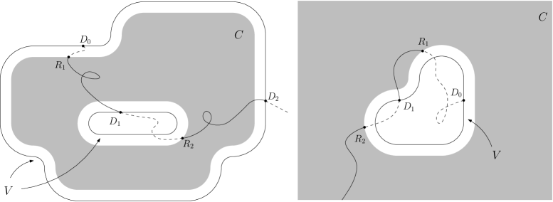
Figure 3: Typical examples of sets $C$ (gray) and $V$ (closed curves). On the left $C$ is finite, while on the right it has finite complement. The stopping times $R_{k}$ and $D_{k}$ are also pictured.

Given a trajectory $w_{+}\in W_{+}$ (recall (2.2)), let us define its successive return and departure times between $C$ and $V$:

$$D_{0} =0,\qquad R_{1}=H_{C},$$

$$D_{1} =H_{V}\circ\theta_{R_{1}}+R_{1},\qquad R_{2}=H_{C}\circ\theta_{D_{1}}+D_{1},$$

$$D_{2} =H_{V}\circ\theta_{R_{2}}+R_{2}\qquad$$ and so on, see Figure 3.

Note that above we have omitted the dependence on $w_{+}$. Define,

$$T^{C}=\inf\{k\geq 1;R_{k}=\infty\},$$ (5.12)

which is equal to one plus the random number of excursions performed by $w_{+}$ until escaping to infinity. Since we assumed the set $V$ to be finite and the random walk on $\mathbb{Z}^{d}$ ($d\geq 3$) is transient, $T^{C}$ is finite $P$-almost surely.

The reason why we define $T^{C}$ as one plus the number of excursions is to guarantee that it coincides with $T_{\Delta}$ as defined just after (4.17) in the construction that follows.

As mentioned before, we are interested in the intersection of $\mathcal{I}^{u}_{V,+}$ (recall (5.6)) with the set $C$. Writing $\chi^{+}_{V,u}=\sum_{j=1}^{\Theta^{V}_{u}}\delta_{w_{j}}$ (where the $w$’s are ordered according to their corresponding $u$’s), and abbreviating $T_{j}^{C}=T^{C}(w_{j})$, we obtain

$$C\cap\mathcal{I}^{u}_{V,+}=C\;\;\cap\quad\bigcup_{\mathchoice{\hbox to0.0pt{\hss$\displaystyle{(w_{+},u)\in\,\operatorname{supp}(\chi^{+}_{V,u})}$\hss}}{\hbox to0.0pt{\hss$\textstyle{(w_{+},u)\in\,\operatorname{supp}(\chi^{+}_{V,u})}$\hss}}{\hbox to0.0pt{\hss$\scriptstyle{(w_{+},u)\in\,\operatorname{supp}(\chi^{+}_{V,u})}$\hss}}{\hbox to0.0pt{\hss$\scriptscriptstyle{(w_{+},u)\in\,\operatorname{supp}(\chi^{+}_{V,u})}$\hss}}}\;\;\operatorname{Range}(w_{+})=C\cap\bigcup_{j=1}^{\Theta^{V}_{u}}\bigcup_{k=1}^{T_{j}^{C}-1}\{X_{R_{k}}(w_{j}),\dots,X_{D_{k}}(w_{j})\},$$ (5.13)

where it may occur that some of the $D_{k}(w_{j})$’s above are infinite.

We are now going to employ the techniques of Section 4 to simulate the above collection of excursions using a Poisson point process. For this let $\Sigma_{C}$ denote the following space of paths

$$\begin{split}\Sigma_{C}=\big{\{}\Delta\big{\}}&\textstyle\bigcup\limits\Big{\{}\begin{array}[]{c}w=(x_{1},\dots,x_{k})\text{ finite nearest neighbor path, starting}\\ \text{at $\partial C$ and ending at its first visit to $V$}\end{array}\Big{\}}\\ &{\textstyle\bigcup}\;\Big{\{}\begin{array}[]{c}w=(x_{1},x_{2},\dots)\text{ infinite nearest neighbor path,}\\ \text{starting at $\partial C$ and never visiting $V$}\end{array}\Big{\}},\end{split}$$ (5.14)

where $\Delta$ is a distinguished state that encodes the fact that a given trajectory has already diverged to infinity. Illustrations of finite and infinite paths in $\Sigma_{C}$ can be found in Figure 3.

Consistently with the previous discussion, we use the shorthand $X^{j}_{\cdot}=X_{\cdot}^{\vphantom{j}}(w_{j})$; in other words, the superscript $j$ means that we are dealing with the $j$th walk of the construction. The excursions induced by the random walks will be encoded as elements of $\Sigma_{C}$ as follows

$$\begin{split}&Z^{j}_{k}=\big{(}X_{R_{k}}^{j},\ldots,X^{j}_{D_{k}}\big{)}\in\Sigma_{C},\text{ for $k=1,\dots,T_{j}^{C}-1$, and}\\ &Z^{j}_{T_{j}^{C}}=\Delta.\end{split}$$ (5.15)

The reason why we introduce the state $\Delta$ is to recover the description of Section 4, indicating that another trajectory is about to start.

In view of (5.13), in order to simulate $C\cap\mathcal{I}^{u}_{V,+}$, we only need to construct the excursions $Z^{j}_{k}$ with the correct law. For this, we are going to use the construction of the previous section to simulate them from a Poisson point process. In (5.18) below, we will prove that for a fixed $j$, the sequence $Z^{j}_{1}$, $Z^{j}_{2}$, $\dots$ is a Markov chain, as required in (4.27) and (4.28).

Endow the space of paths $\Sigma_{C}$ with the $\sigma$-algebra $\mathcal{S}$ generated by the canonical coordinates and with the measure $\mu_{C}$ given by

$$\mu_{C}(\mathcal{X})=\sum_{x\in\partial C}P_{x}\big{[}(X_{0},X_{1},\dots,X_{H_{V}})\in\mathcal{X}\big{]}+\delta_{\Delta}(\mathcal{X}),$$ (5.16)

where $\mathcal{X}\in\mathcal{S}$. Note that $\mu_{C}$ is finite due to (5.11). We can therefore define a Poisson point process $\eta=\sum_{i}\delta_{(z_{i},v_{i})}$ on $\Sigma_{C}\times\mathbb{R}_{+}$ with intensity $\mu_{C}\otimes\mathrm{d}v$ as in (4.1).

In order to apply Proposition 4.10, we first observe that for fixed $j\geq 1$, $Z^{j}_{k}$ is a Markov chain, due to the Markovian character of the simple random walk. We then define

$$f^{C}_{y}(x):=P_{y}[X_{\tilde{H}_{C}}=x]$$ (5.17)

and apply the strong Markov property at $D_{k-1}$, to obtain the Radon-Nikodym derivative

$$\frac{\mathrm{d}P[Z^{j}_{k}\in\cdot\mid Z^{j}_{k-1}=z]}{\mathrm{d}\mu_{C}}(z^{\prime})=\begin{cases}1,&\text{ if $z=z^{\prime}=\Delta$,}\\ &\text{ or $z^{\prime}=\Delta,D_{k-1}=\infty$,}\\ f^{C}_{X^{j}_{D_{k-1}}(z)}\big{(}X_{0}(z^{\prime})\big{)},&\text{ if $z,z^{\prime}\neq\Delta$, $D_{k-1}<\infty$,}\\ \smash{P_{X^{j}_{D_{k-1}}(z)}}[H_{C}=\infty],&\text{ if $z^{\prime}=\Delta\neq z$, $D_{k-1}<\infty$,}\\ 0,&\text{ otherwise,}\end{cases}$$ (5.18)

for all $k\geq 2$.

Not only the above shows that the sequence $Z^{j}_{1},Z^{j}_{2},\dots$ is Markovian, but also that the transition density of the chain satisfies

$$g_{C}\big{(}(x_{0},\dots,x_{l}),(y_{0},\dots,y_{m})\big{)}=f_{x_{l}}(y_{0})$$ (5.19)

($g$ is a density with respect to $\mu_{C}$, as in (5.16)). We are now left with the starting distributions of the Markov chains $Z^{j}_{k}$.

Recall that we are attempting to construct the measure $\chi^{+}_{V,u}$, which is not independent of $\chi^{-}_{V,u}$. In fact, they are conditionally independent given $\{X_{0}(w)\}_{w\in\operatorname{supp}(\chi^{-}_{V,u})}$. Therefore, conditioning on $\{X^{j}_{0}\}_{j=1,\dots,\Theta^{V}_{u}}$, the starting density of the $j$-th chain (with respect to $\mu_{C}$) satisfies

$$g^{j}_{C}(x_{0},\dots,x_{l})=f_{X^{j}_{0}}(x_{0}).$$ (5.20)

Finally, we set $Z^{j}_{0}=w$ where $w$ is any trajectory with $X_{0}(w)=X^{j}_{0}=X^{j}_{D_{0}}$, so that (5.18) is also satisfied for $k=1$, in compliance with the notation in (4.27) (see also Remark 4.7).

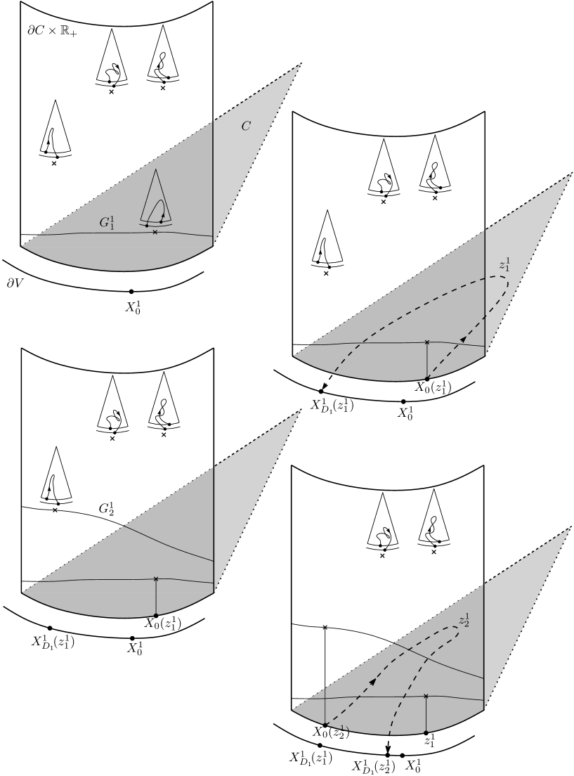
Figure 4: On the construction of random interlacements on the set $C$; the points of $\Sigma_{C}$ are substituted by points in $\partial C\times\mathbb{R}_{+}$ with marks representing the corresponding trajectories, and the state $\Delta$ is not pictured

We can now follow the construction of $\xi^{C}_{j,k}$ and $G^{C}_{j,k}$, for $j\geq 1$, $k=1,\dots,T^{C}_{j}$, as in (4.31). Then, using Proposition 4.10, we obtain a way to simulate the excursions $Z^{j}_{k}$ as promised. In particular, we can show that

$$C\cap\mathcal{I}^{u}_{V,+}\text{ is distributed as $C\cap\bigcup_{j=1}^{\Theta^{V}_{u}}\bigcup_{k=1}^{T^{C}_{j}}\operatorname{Range}(z^{C}_{j,k})$ under $\mathbb{Q}$.}$$ (5.21)

See on Figure 4 an illustration of the first two steps (for the first particle) of the construction of random interlacements on the set $C$.

We now prove a proposition that relates our main result Theorem 2.1 with the above construction. To simplify the notation for the soft local time, we abbreviate the accumulated soft local time up to the $\Theta^{C}_{u}$-th trajectory

$$G^{C}_{u}=G^{C}_{1,T^{C}_{1}}+G^{C}_{2,T^{C}_{2}}+\cdots+G^{C}_{\Theta^{C}_{u},T^{C}_{\Theta^{C}_{u}}}.$$ (5.22)

We can use Theorem 4.6 to obtain a short expression for $EG^{C}_{v}(z)$. For this, given $j\geq 1$, we let

$$\rho^{C}_{j}(x)=\sum_{k=1}^{T_{j}^{C}}1_{x}(X^{j}_{R_{k}})$$ (5.23)

count the number of times the $j$-th trajectory starts an excursion through $x$.

Let us first recall, from (5.19), that $G^{C}_{v}$ depends on $z=(x_{0},x_{1},\dots)$ solely through $x_{0}$. Thus, given $z,z^{\prime}\in\Sigma_{C}$, we define $q(z,z^{\prime})=1\{X_{0}(z)=X_{0}(z^{\prime})\}$ to obtain that

$$\begin{array}[]{e}E^{\mathbb{Q}}G^{C}_{1,T_{1}^{C}}(z)&\overset{\eqref{e:gtrans}}{=}&\int q(z,z^{\prime})E^{\mathbb{Q}}G^{C}_{1,T_{1}^{C}}(z^{\prime})\,\mu_{C}(\mathrm{d}z^{\prime})\\ \hfil&\overset{\mathchoice{\hbox to0.0pt{\hss$\displaystyle{\text{Theorem~{}\ref{t:expectsingle}}}$\hss}}{\hbox to0.0pt{\hss$\textstyle{\text{Theorem~{}\ref{t:expectsingle}}}$\hss}}{\hbox to0.0pt{\hss$\scriptstyle{\text{Theorem~{}\ref{t:expectsingle}}}$\hss}}{\hbox to0.0pt{\hss$\scriptscriptstyle{\text{Theorem~{}\ref{t:expectsingle}}}$\hss}}}{=}&\qquad E^{\mathcal{P}}\Big{(}\sum_{k=1}^{T^{C}_{j}}q(Z^{j}_{k},z)\Big{)}=E^{\mathcal{P}}\rho^{C}_{j}(X_{0}(z)),\end{array}$$ (5.24)

for every $z\in\Sigma_{C}$. Clearly, this implies that

$$E^{\mathbb{Q}}G^{C}_{v}(z)=E^{\mathbb{Q}}\Theta^{C}_{v}\times E^{\mathcal{P}}\rho^{C}_{j}(X_{0}(z))=v\operatorname{cap}(V)E^{\mathcal{P}}\rho^{C}_{j}(X_{0}(z)).$$ (5.25)

Proposition 5.3.

Let $A_{1}$ and $A_{2}$ be two disjoint subsets of $\mathbb{Z}^{d}$ with $A_{2}$ having finite complement. Now suppose that

$$\begin{array}[]{c}\text{$V\subset\mathbb{Z}^{d}$ is such that any path from $A_{1}$ to $A_{2}$ crosses $V$.}\end{array}$$ (5.27)

Then, for every $u>0$ and $\varepsilon\in(0,1)$ there exists a coupling $\mathbb{Q}$ between $\mathcal{I}^{u}$ and two independent random interlacements processes, $(\mathcal{I}^{u}_{1})_{u\geq 0}$ and $(\mathcal{I}^{u}_{2})_{u\geq 0}$ such that

$$\begin{split}\mathbb{Q}\big{[}&\mathcal{I}^{u(1-\varepsilon)}_{k}\cap A_{k}\;\subseteq\;\mathcal{I}^{u}\cap A_{k}\;\subseteq\;\mathcal{I}^{u(1+\varepsilon)}_{k},\text{ $k=1,2$}\big{]}\\ &\;\;\geq 1-\quad\sum_{\mathchoice{\hbox to0.0pt{\hss$\displaystyle{\begin{subarray}{c}(v,C)=(u(1\pm\varepsilon),A_{1}),\\ (u(1\pm\varepsilon),A_{2}),(u,A_{1}\cup A_{2})\end{subarray}}$\hss}}{\hbox to0.0pt{\hss$\textstyle{\begin{subarray}{c}(v,C)=(u(1\pm\varepsilon),A_{1}),\\ (u(1\pm\varepsilon),A_{2}),(u,A_{1}\cup A_{2})\end{subarray}}$\hss}}{\hbox to0.0pt{\hss$\scriptstyle{\begin{subarray}{c}(v,C)=(u(1\pm\varepsilon),A_{1}),\\ (u(1\pm\varepsilon),A_{2}),(u,A_{1}\cup A_{2})\end{subarray}}$\hss}}{\hbox to0.0pt{\hss$\scriptscriptstyle{\begin{subarray}{c}(v,C)=(u(1\pm\varepsilon),A_{1}),\\ (u(1\pm\varepsilon),A_{2}),(u,A_{1}\cup A_{2})\end{subarray}}$\hss}}}\quad\mathbb{Q}\Big{[}\big{|}G^{C}_{v}(z)-E^{\mathbb{Q}}G^{C}_{v}(z)\big{|}\geq\tfrac{\varepsilon}{3}E^{\mathbb{Q}}G^{C}_{v}(z)\text{ for some $z\in\Sigma_{C}$}\Big{]},\end{split}$$ (5.28)

where the soft local times above are determined in terms of $V$.

We note that the above proposition is an important ingredient for the proof of Theorem 2.1, since it relates the success probability of our decoupling with an estimate on the soft local times. In Section 6, we will bound the right hand side of (5.28) using large deviations. One should not be worried that the set $\Sigma_{C}$ may be uncountable (in case the excursions are infinite). Later we will deal with this using the fact that the soft local time depends on $z$ only through its starting point.

Proof.

We are going to follow the scheme in Section 5.1 in order to construct the triple $\mathcal{I}^{u}$, $(\mathcal{I}^{u}_{1})_{u\geq 0}$ and $(\mathcal{I}^{u}_{2})_{u\geq 0}$, distributed as random interlacements on $\mathbb{Z}^{d}$ as stated in the proposition. However, we will need two independent copies of some of the ingredients appearing in that construction. More precisely,

let $$\chi^{-}_{V,1}=\textstyle\sum_{i}\delta_{(w^{1}_{i},u^{1}_{i})} \chi^{-}_{V,2}=\textstyle\sum_{i}\delta_{(w^{2}_{i},u^{2}_{i})} M \chi^{-}_{V}$$ and be two independent random variables on (i.e., Poisson point processes on the space of labelled trajectories) with the same law as in (5.4), (5.29)

let the counting process $$\Theta^{V,1}_{u}=\chi^{-}_{V,1}(W_{+}\times[0,u]) \Theta^{V,2}_{u}=\chi^{-}_{V,2}(W_{+}\times[0,u]) u\geq 0$$ and be as in (5.10), for , and finally (5.30)

define two independent processes $$\widehat{\mathcal{I}}^{u}_{V,1} \widehat{\mathcal{I}}^{u}_{V,2}$$ and as in (5.6). (5.31)

The only missing ingredients in order to construct two independent random interlacements processes following the construction of Section 5.1 are the random walks composing $\chi^{+}_{V}$, see (5.4). Such construction will be based on Proposition 4.10 and that is where the coupling will take place.

Let us introduce the sets

$$\begin{array}[]{c}\text{$\Sigma_{A_{1}\cup A_{2}}$, $\Sigma_{A_{1}}$ and $\Sigma_{A_{2}}$ given by~{}\eqref{e:Sigma} with $V$ as in \eqref{e:aPsi}.}\end{array}$$ (5.32)

Note that we have replaced the set $C$ by the three above choices, while keeping $V$ fixed.

We also let $\mu_{A_{1}\cup A_{2}}$, $\mu_{A_{1}}$ and $\mu_{A_{2}}$ be the respective measures on these sets, given by (5.16). The first crucial observation for this proof is the fact that

$$\begin{array}[]{c}\Sigma_{A_{1}\cup A_{2}}\text{ is the disjoint union of $\Sigma_{A_{1}}$ and $\Sigma_{A_{2}}$ and $\mu_{A_{1}\cup A_{2}}=\mu_{A_{1}}+\mu_{A_{2}}$}.\end{array}$$ (5.33)

Note that we are duplicating the cemetery on $\Sigma_{A_{1}\cup A_{2}}$, for the above to hold.

We define a Poisson point process $\eta$ on $\Sigma_{A_{1}\cup A_{2}}\times\mathbb{R}_{+}$ with intensity $\mu_{A_{1}\cup A_{2}}\otimes\mathrm{d}v$ as below (5.16). From (5.33) we conclude that,

$$\begin{array}[]{c}\text{$\eta$ restricted to $\Sigma_{A_{1}}$ and $\Sigma_{A_{2}}$ are Poisson point processes with respective}\\ \text{intensities $\mu_{A_{1}}\otimes\mathrm{d}v$ and $\mu_{A_{2}}\otimes\mathrm{d}v$, which are independent of each other.}\\ \text{Moreover, an excursion $z\in\Sigma_{A_{k}}$ cannot intersect $A_{k^{\prime}}$ with $k\neq k^{\prime}$, see \eqref{e:aPsi}.}\end{array}$$ (5.34)

We use $\chi^{-}_{V,1}$ and $\chi^{-}_{V,2}$ in order to define the starting points $\{X^{V,1,j}_{0}\}_{j=1,\dots,\Theta^{A_{1}}_{u}}$ and $\{X^{V,2,j}_{0}\}_{j=1,\dots,\Theta^{A_{2}}_{u}}$. Let us finally recall the definitions of $T^{C}$ from (5.12), $G^{C}_{j,k}$ and $z^{C}_{j,k}$ from (4.31), where $C$ can be replaced by either of the three sets $(A_{1}\cup A_{2})$, $A_{1}$, or $A_{2}$. It is important to observe that we use the starting points $X^{V,1,j}_{0}$ for the case $C=A_{1}$ and $X^{V,2,j}_{0}$ for both $C=A_{2}$ or $(A_{1}\cup A_{2})$. We can finally introduce

$$\mathcal{J}^{u}_{C}=C\cap\bigcup_{j=1}^{\Theta^{C}_{u}}\bigcup_{k=1}^{T^{C}_{j}}\operatorname{Range}\big{(}z^{C}_{j,k}\big{)},\text{ with $C=(A_{1}\cup A_{2})$, $A_{1}$ or $A_{2}$}$$ (5.35)

(note that we use the same Poisson point process to define the three sets above) and

$$\mathcal{I}^{u} =\mathcal{J}^{u}_{(A_{1}\cup A_{2})}\cup\mathcal{I}^{u}(\chi^{-}_{V,2})\cup\widehat{\mathcal{I}}^{u}_{V,2},$$

$$\mathcal{I}^{u}_{1} =\mathcal{J}^{u}_{A_{1}}\cup\mathcal{I}^{u}(\chi^{-}_{V,1})\cup\widehat{\mathcal{I}}^{u}_{V,1},\text{ and}$$

$$\mathcal{I}^{u}_{2} =\mathcal{J}^{u}_{A_{2}}\cup\mathcal{I}^{u}(\chi^{-}_{V,2})\cup\widehat{\mathcal{I}}^{u}_{V,2}.$$

We independently modify the above sets on $(A_{1}\cup A_{2})^{c}$ to obtain the correct distributions, although this is immaterial for the statement of the proposition.

To conclude the proof of the proposition, let us observe that

• $(\mathcal{J}^{u}_{C})_{u\geq 0}$ is distributed as $(C\cap\mathcal{I}^{u}_{V,+})_{u\geq 0}$, for $C=(A_{1}\cup A_{2})$, $A_{1}$ or $A_{2}$, see (5.21), so that $((A_{1}\cup A_{2})\cap\mathcal{I}^{u})_{u\geq 0}$, $(A_{1}\cap\mathcal{I}^{u}_{1})_{u\geq 0}$ and $(A_{2}\cap\mathcal{I}^{u}_{2})_{u\geq 0}$ have the right distributions as under the random interlacements;

• $\mathcal{J}^{u}_{A_{1}}$ and $\mathcal{J}^{u}_{A_{2}}$ are independent, see (5.29), (5.30) and (5.34), which means that $(A_{1}\cap\mathcal{I}^{u}_{1})_{u\geq 0}$ and $(A_{2}\cap\mathcal{I}^{u}_{2})_{u\geq 0}$ are also independent.

So that, using the definition of $\mathcal{I}^{u}$, $\mathcal{I}^{u}_{1}$ and $\mathcal{I}^{u}_{2}$,

$$\mathbb{Q}\big{[}\mathcal{I}^{u(1-\varepsilon)}_{k} \cap A_{k}\;\subseteq\;\mathcal{I}^{u}\cap A_{k}\;\subseteq\mathcal{I}^{u(1+\varepsilon)}_{k},\text{ $k=1,2$}\big{]}$$

$$\geq\mathbb{Q}\big{[}\mathcal{J}^{u(1-\varepsilon)}_{A_{k}}\subseteq\;\mathcal{J}^{u}_{A_{1}\cup A_{2}}\cap A_{k}\;\subseteq\mathcal{J}^{u(1+\varepsilon)}_{A_{k}},\text{ $k=1,2$}\big{]}$$ (5.36)

$$\geq\mathbb{Q}\big{[}G^{A_{k}}_{u(1-\varepsilon)}(z)\leq G^{A_{1}\cup A_{2}}_{u}(z)\leq G^{A_{k}}_{u(1+\varepsilon)}(z),\text{ for all $z\in\Sigma_{A_{k}}$ and $k=1,2$}\big{]}.$$

Now, (5.27) implies that for $x\in\partial A_{k}$ we have $\varphi(x):=E^{\mathcal{P}}\rho^{A_{k}}_{1}(x)=E^{\mathcal{P}}\rho^{A_{1}\cup A_{2}}_{1}(x)$. The conclusion of (5.28) is now a simple consequence of the above display and the fact that the expectation of $G^{C}_{u}$ is linear in $u$ according to (5.25) (see Figure 5).

Figure 5: On the proof of Proposition 5.3, $\varphi$ was defined in the last paragraph of the proof (observe that $1+\frac{\varepsilon}{3}\leq(1-\frac{\varepsilon}{3})(1+\varepsilon)$ for $\varepsilon\in[0,1]$)

∎

6 Proof of Theorem 2.1

In this section we will prove our main result, modulo a set of additional assumptions that will be proved in the next section.

Recall that we use the notation $B(x,r)=\{y\in\mathbb{Z}^{d}:\|x-y\|\leq r\}$ for discrete balls. Also, for $A\subset\mathbb{Z}^{d}$ we write $B(A,r)=\bigcup_{x\in A}B(x,r)$.

Suppose we are given sets $A_{1}$ and $A_{2}$ as in Theorem 2.1 and suppose without loss of generality that the diameter of $A_{1}$ is not greater than the diameter of $A_{2}$. It is clear that we can assume that $A_{2}=\mathbb{Z}^{d}\setminus B(A_{1},s)$, since the function $f_{2}$ can be seen as a function in $\{0,1\}^{\mathbb{Z}^{d}\setminus B(A_{1},s)}$; so, from now on we work with this assumption.

The proof of the main theorem will require some estimates on the entrance distribution of a random walk on the sets $A_{1}$, $A_{2}$ and $A_{1}\cup A_{2}$, which are closely related to the regularity conditions mentioned above Theorem 4.9. However, the problem is that, in general, these estimates need not be satisfied for arbitrary finite set $A_{1}$ and $A_{2}=\mathbb{Z}^{d}\setminus B(A_{1},s)$. So, in order to fix this problem, we will replace $A_{1}$ and $A_{2}$ by slightly larger sets $A^{(s)}_{1}$ and $A^{(s)}_{2}$, using Proposition 6.1 below. Roughly speaking, these “fattened” sets will have the following properties (below, $C$ stands for any of the three sets $A^{(s)}_{1},A^{(s)}_{2},$ or $A^{(s)}_{1}\cup A^{(s)}_{2}$):

• the probability that the simple random walk enters $C$ through some point $y$ is at most $O(s^{-(d-1)})$, for starting points at distance at least of order $s$ from $C$;

• this probability should be at least of order $s^{-(d-1)}$ for “many” starting points which are at distance of order $s$ from $y$;

• the probabilities of entering $C$ through two near points $y$ and $y^{\prime}$ in $\partial C$ can be different by at most a (fixed) constant factor (this should be valid as soon as the random walk starts far from $\{y,y^{\prime}\}$);

• finally, we also need some additional geometric properties of $\partial C$.

A typical example of a set having these properties is a discrete ball of radius $s$; in fact, we will prove that any set with “sufficiently smooth boundary” will do. More rigorously, the fact that we need is formulated in the following way (one may find helpful to look at Figure 6):

Proposition 6.1.

There exist positive constants $\gamma_{\textnormal{\tiny\ref{regular}}}\in(0,\frac{1}{10})$, $\gamma_{\textnormal{\tiny\ref{reg2}}}$, $\gamma_{\textnormal{\tiny\ref{reg8}}}<\frac{\gamma_{\textnormal{\tiny\ref{regular}}}}{2}$, $\gamma_{\textnormal{\tiny\ref{reg9}}},\gamma_{\textnormal{\tiny\ref{reg10}}},\gamma_{\textnormal{\tiny\ref{reg11}}}\in(0,1),s_{0}$ (depending only on dimension) such that, for any $s\geq s_{0}$ and any set $A\subset\mathbb{Z}^{d}$ such that $\mathbb{Z}^{d}\setminus B(A,s)$ is nonempty, there is a set $A^{(s)}$ with the following properties:

$$A\subseteq A^{(s)}\subseteq B\Big{(}A,\frac{s}{5}\Big{)};$$ (6.1)

for any $$y\in\partial A^{(s)}$$,

$$\sup_{\begin{subarray}{c}x\in\mathbb{Z}^{d};\\ \operatorname{d}(x,y)\geq\gamma_{\textnormal{\tiny\ref{regular}}}s/2\end{subarray}}P_{x}[X_{H_{A^{(s)}}}=y]\leq\gamma_{\textnormal{\tiny\ref{reg2}}}s^{-(d-1)}$$ (6.2)

and there exists a ball $$\bar{B}_{y} \gamma_{\textnormal{\tiny\ref{regular}}}s \operatorname{d}(\bar{B}_{y},y)\in[\gamma_{\textnormal{\tiny\ref{regular}}}s,2\gamma_{\textnormal{\tiny\ref{regular}}}s]$$ of radius such that and

$$\inf_{x\in\bar{B}_{y}}P_{x}[X_{H_{A^{(s)}}}=y,H_{A^{(s)}}<H_{\mathbb{Z}^{d}\setminus B(y,4\gamma_{\textnormal{\tiny\ref{regular}}}s)}]\geq\gamma_{\textnormal{\tiny\ref{reg2}}}^{-1}s^{-(d-1)}.$$ (6.3)

Moreover, for any $$y\in\partial A^{(s)}$$

$$|\{z\in\partial A^{(s)}:\|y-z\|\leq\gamma_{\textnormal{\tiny\ref{reg8}}}s\}|\geq\gamma_{\textnormal{\tiny\ref{reg9}}}s^{d-1}$$ (6.4)

and if $$y^{\prime}\in\partial A^{(s)} \|y-y^{\prime}\|\leq\gamma_{\textnormal{\tiny\ref{reg8}}}s \hat{D} y,y^{\prime} \{y,y^{\prime}\} \partial B(y,\gamma_{\textnormal{\tiny\ref{regular}}}s) \partial B(y,\gamma_{\textnormal{\tiny\ref{regular}}}s) A^{(s)} \{y,y^{\prime}\} \hat{D}$$ is such that , then there exists a set (depending on ) that separates from (i.e., any nearest-neighbor path starting at that enters at , must pass through ) such that

$$\sup_{\begin{subarray}{c}x\in\hat{D};\\ P_{x}[X_{H_{\!A^{(s)}}}=y^{\prime}]>0\end{subarray}}\frac{P_{x}[X_{H_{A^{(s)}}}=y]}{P_{x}[X_{H_{A^{(s)}}}=y^{\prime},H_{A^{(s)}}<H_{\mathbb{Z}^{d}\setminus B(y^{\prime},5\gamma_{\textnormal{\tiny\ref{regular}}}s)}]}\leq\gamma_{\textnormal{\tiny\ref{reg10}}}.$$ (6.5)

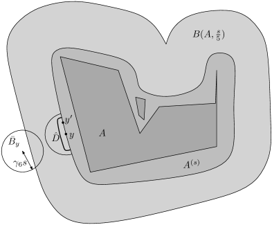
Figure 6: On the sets in Proposition 6.1

The proof of this proposition is postponed to Section 8. We now are going to use the above result to prove Theorem 2.1.

Recall that we define $A_{2}=\mathbb{Z}^{d}\setminus B(A_{1},s)$. The idea is to use Proposition 5.3 for $A_{1}^{(s)}$ and $A_{2}^{(s)}$ provided by Proposition 6.1, and $V$ defined as

$$V=\big{\{}y\in\mathbb{Z}^{d}:\operatorname{d}(y,A_{1}^{(s)}\cup A_{2}^{(s)})\geq\gamma_{\textnormal{\tiny\ref{regular}}}s\big{\}}.$$ (6.6)

Let $y,y^{\prime}\in\partial A_{1}^{(s)}\cup\partial A_{2}^{(s)}$ be such that $\|y-y^{\prime}\|\leq\gamma_{\textnormal{\tiny\ref{reg8}}}s$ (in fact, in this case both $y$ and $y^{\prime}$ must be in the same set, either $\partial A_{1}^{(s)}$ or $\partial A_{2}^{(s)}$). Let $\hat{D}$ be the corresponding separating set, as in (6.5) of Proposition 6.1. Now, consider an arbitrary site $x\in V$, and write for $C=A_{1}^{(s)},A_{2}^{(s)},A_{1}^{(s)}\cup A_{2}^{(s)}$

$$P_{x}[X_{H_{C}}=y]=\sum_{z\in\hat{D}}P_{x}[X_{H_{C\cup\hat{D}}}=z]P_{z}[X_{H_{C}}=y]\text{ and similarly with $y^{\prime}$},$$ (6.7)

where we used the strong Markov property at $H_{C\cup\hat{D}}$ and dropped vanishing terms. So, by construction, we have

$$\sup_{\begin{subarray}{c}x\in V;\\ P_{x}[X_{H_{C}}=y^{\prime}]>0\end{subarray}}\frac{P_{x}[X_{H_{C}}=y]}{P_{x}[X_{H_{C}}=y^{\prime}]}\leq\gamma_{\textnormal{\tiny\ref{reg10}}}\quad\text{ for }C=A_{1}^{(s)},A_{2}^{(s)},A_{1}^{(s)}\cup A_{2}^{(s)},\text{ when }\|y-y^{\prime}\|\leq\gamma_{\textnormal{\tiny\ref{reg8}}}s.$$ (6.8)

With the above, we can now start estimating the soft local times appearing in (5.28).

In the rest of this section, $C$ stands for one of the sets $A_{1}^{(s)},A_{2}^{(s)},A_{1}^{(s)}\cup A_{2}^{(s)}$; we will obtain the same estimates for all of them. Recalling the definition of $T_{\ell}$ in (4.21), we consider $x\in\partial C$ and fix any $z\in\Sigma_{C}$ such that $x=X_{0}(z)$; then we denote

$$F^{C}_{j}(x)=G^{C}_{j,T^{C}_{j}}(z)$$ (6.9)

to be the contribution of the $j$-th particle to the soft local time in trajectories starting at $x$, in the construction of the corresponding interlacement set for $C$, so that $G^{C}_{u}(z)=\sum_{j=1}^{\Theta^{C}_{u}}F^{C}_{j}(x)$.

We also introduce

$$\pi^{C}(x)=E[F^{C}_{1}(x)],\text{ which also equals $E^{\mathcal{P}}\rho_{1}^{C}(x)$ due to \eqref{e:EGisErho},}$$ (6.10)

recall the definition of $\rho^{C}_{j}$ from (5.23).

Lemma 6.2.

For $C$ being either $A_{1}^{(s)}$, $A_{2}^{(s)}$ or $A_{1}^{(s)}\cup A_{2}^{(s)}$ and $V$ as in (6.6), we have for all $x\in\partial C$

• $\gamma_{\textnormal{\tiny\ref{c:L41'}}}s^{-1}\operatorname{cap}(V)^{-1}\leq\pi^{C}(x)\leq\gamma_{\textnormal{\tiny\ref{c:L41''}}}s^{-1}\operatorname{cap}(V)^{-1}\vphantom{\displaystyle\int}$;

• $E(F_{1}^{C}(x))^{2}\leq\gamma_{\textnormal{\tiny\ref{c:L41'''}}}s^{-d}\operatorname{cap}(V)^{-1}\vphantom{\displaystyle\sum}$.

Proof.

Instead of estimating the expected soft local time directly, we rather work with the “real” local time $\rho_{1}^{C}(x)$, with the assistance of Theorem 4.6.

Consider the discrete sphere $\tilde{V}$ of radius $3(r+s)$ centered in any fixed point of $A_{1}$. Given a trajectory $w^{*}\in W^{*}$, the number of excursions $\rho_{1}^{C}(x)$ between $V$ and $C$ entering at $x$ is the same for both $s_{V}(w^{*})$ and $s_{\tilde{V}}(w^{*})$. Thus, their expected values are the same and can be written respectively as $u\operatorname{cap}(V)\pi^{C}(x)$ and $u\operatorname{cap}(\tilde{V}){\tilde{\pi}}^{C}(x)$, where ${\tilde{\pi}}^{C}(x)$ is the expected number of such $(V,x)$-crossings under $P_{\bar{e}_{\tilde{V}}}$. So,

$$\pi^{C}(x)=\operatorname{cap}(V)^{-1}\operatorname{cap}(\tilde{V}){\tilde{\pi}}^{C}(x).$$

We know that $\operatorname{cap}(\tilde{V})\asymp(r+s)^{d-2}$ (see (2.8)), so, in order to prove the part (i), it will be enough to obtain that

$${\tilde{\pi}}^{C}(x)\asymp s^{-1}(r+s)^{-(d-2)}.$$ (6.11)

For $x^{\prime}\in\mathbb{Z}^{d}\setminus C$ such that $d(x^{\prime},x)\geq\gamma_{\textnormal{\tiny\ref{regular}}}s$, we use the Markov property at $H_{C}$ to obtain

$$E_{x^{\prime}}\rho_{1}^{C}(x)\leq P_{x^{\prime}}[X_{H_{C}}=x]+\sup_{y\in V}P_{y}[H_{B(x,\gamma_{\textnormal{\tiny\ref{regular}}}s/2)}<\infty]\sup_{z:d(z,x)\geq\gamma_{\textnormal{\tiny\ref{regular}}}s/2}E_{z}\rho_{1}^{C}(x).$$ (6.12)

Then taking the supremum in $x^{\prime}$ and using (6.2), we get that

$$\sup_{x^{\prime}:d(x^{\prime},x)\geq\gamma_{\textnormal{\tiny\ref{regular}}}s/2}E_{x^{\prime}}\rho_{1}^{C}(x)\leq\frac{\sup_{x^{\prime}:d(x^{\prime},x)\geq\gamma_{\textnormal{\tiny\ref{regular}}}s/2}P_{x^{\prime}}[X_{H_{C}}=x]}{1-\sup_{y\in V}P_{y}[H_{B(x,\gamma_{\textnormal{\tiny\ref{regular}}}s/2)}<\infty]}\leq c_{\textnormal{\tiny\ref{c:p24}}}s^{-(d-1)}.$$ (6.13)

So, by Proposition 6.4.2 of [10],

$$E_{\bar{e}_{\tilde{V}}}\rho_{1}^{C}(x) \leq\sup_{x^{\prime}\in{\tilde{V}}}P_{x^{\prime}}[H_{B(x,\gamma_{\textnormal{\tiny\ref{regular}}}s/2)}<\infty]\sup_{x^{\prime}:d(x^{\prime},x)\geq\gamma_{\textnormal{\tiny\ref{regular}}}s/2}E_{x^{\prime}}\rho_{1}^{C}(x)$$

$$\leq c_{\textnormal{\tiny\ref{c:p24'}}}\Big{(}\frac{s}{s+r}\Big{)}^{-(d-2)}s^{-(d-1)}=c_{\textnormal{\tiny\ref{c:p24'}}}s^{-1}(r+s)^{-(d-2)}.$$

We are now left with the lower bound

$$E_{\bar{e}_{\tilde{V}}}\rho_{1}^{C}(x)\geq\inf_{x^{\prime}\in\partial\tilde{V}}P_{x^{\prime}}[H_{\bar{B}_{x}}<\infty]\inf_{x^{\prime\prime}\in\partial\bar{B}_{x}}P_{x^{\prime\prime}}[X_{H_{C}}=x]\overset{\eqref{hip3}}{\geq}c_{\textnormal{\tiny\ref{c:p24''}}}\Big{(}\frac{s}{s+r}\Big{)}^{-(d-2)}s^{-(d-1)},$$

proving (6.11) and consequently (i).

The part (ii) then immediately follows from (6.13) and Theorem 4.8 (see also Remark 4.7). ∎

Next, we need the following large deviation bound for $F_{1}^{C}(x)$:

Lemma 6.3.

For $C=A_{1}^{(s)},A_{2}^{(s)},A_{1}^{(s)}\cup A_{2}^{(s)}$ and $V$ as in (6.6), we have for all $x\in\partial C$

$$P[F_{1}^{C}(x)>v\gamma_{\textnormal{\tiny\ref{reg2}}}s^{-(d-1)}]\leq\gamma_{\textnormal{\tiny\ref{c:L42'}}}s^{d-2}\operatorname{cap}(V)^{-1}\exp(-\gamma_{\textnormal{\tiny\ref{c:L42''}}}v),\text{ for any $v\geq 2$}$$ (6.14)

(also, without loss of generality we suppose that $\gamma_{\textnormal{\tiny\ref{c:L42''}}}\leq 1$).

Proof.

The idea is to apply Theorem 4.9 for $F_{1}^{C}(x)$ and with $\Gamma_{x}=\{z\in\Sigma_{C}:\|x-X_{0}(z)\|\leq\gamma_{\textnormal{\tiny\ref{reg8}}}s\}$; observe that $\mu_{C}(\Gamma_{x})\geq\gamma_{\textnormal{\tiny\ref{reg9}}}s^{d-1}$ by (6.4). With the notation of Theorem 4.9, we set

$$\ell=\gamma_{\textnormal{\tiny\ref{reg2}}}s^{-(d-1)}\quad\text{ and observe that }\quad\alpha\geq\frac{1}{\gamma_{\textnormal{\tiny\ref{reg10}}}},$$

by (6.2) and (6.8).

Chebyshev’s inequality together with Lemma 6.2 (i) then imply that

$$P[T_{\ell}<\infty]=P[F_{1}^{C}(x)\geq\gamma_{\textnormal{\tiny\ref{reg2}}}s^{-(d-1)}]\leq\frac{\pi^{C}(x)}{\gamma_{\textnormal{\tiny\ref{reg2}}}s^{-(d-1)}}\leq\gamma_{\textnormal{\tiny\ref{reg2}}}^{-1}\gamma_{\textnormal{\tiny\ref{c:L41''}}}s^{d-2}\operatorname{cap}(V)^{-1}.$$ (6.15)

Now, denoting by $N(\Gamma_{x})$ the number of crossings between $V$ and $C$ that enter in $\Gamma_{x}$ and by $\eta_{x}$ the number of points of the Poisson process (from the construction in Section 5) in $\Gamma_{x}\times\big{[}0,\frac{\gamma_{\textnormal{\tiny\ref{reg2}}}}{2\gamma_{\textnormal{\tiny\ref{reg10}}}}vs^{-(d-1)}\big{]}$, we write

$$\mathbb{Q}_{z^{\prime}}\big{[}\eta_{x}\leq N(\Gamma_{x})\big{]}\leq\mathbb{Q}_{z^{\prime}}\Big{[}\eta_{x}\leq\frac{\gamma_{\textnormal{\tiny\ref{reg2}}}\gamma_{\textnormal{\tiny\ref{reg9}}}}{4\gamma_{\textnormal{\tiny\ref{reg10}}}}v\Big{]}+\mathbb{Q}_{z^{\prime}}\Big{[}N(\Gamma_{x})\geq\frac{\gamma_{\textnormal{\tiny\ref{reg2}}}\gamma_{\textnormal{\tiny\ref{reg9}}}}{4\gamma_{\textnormal{\tiny\ref{reg10}}}}v\Big{]}.$$

To see that both terms in the right-hand side of the above display are exponentially small in $v$, we observe that

• $\eta_{x}$ has Poisson distribution with parameter at least $\frac{\gamma_{\textnormal{\tiny\ref{reg2}}}\gamma_{\textnormal{\tiny\ref{reg9}}}}{2\gamma_{\textnormal{\tiny\ref{reg10}}}}v$, and

• starting from any $y\in V$, with uniformly positive probability the random walk does not enter in $\Gamma_{x}$ (recall that $\gamma_{\textnormal{\tiny\ref{reg8}}}<\frac{\gamma_{\textnormal{\tiny\ref{regular}}}}{2}$, which implies that $P_{y}[H_{\Gamma_{x}}<\infty]<c_{\textnormal{\tiny\ref{c:unif}}}<1$ uniformly in $y\in V$). Therefore $N_{x}$ is dominated by a Geometric($c_{\textnormal{\tiny\ref{c:unif}}}$) random variable having exponential tail as well.

Together with (6.15) and Theorem 4.9, this finishes the proof of Lemma 6.3. ∎

Now, we are able to finish the proof of our main result.

Proof of Theorem 2.1..

For $C=A_{1},A_{2},A_{1}\cup A_{2}$ and $x\in\partial C$, let $\psi^{x}_{C}(\lambda)=Ee^{\lambda F_{1}^{C}(x)}$ be the moment generating function of $F_{1}^{C}(x)$. It is elementary to obtain that $e^{t}-1\leq t+t^{2}$ for all $t\in[0,1]$. Using this observation, we write for $0\leq\lambda\leq\frac{1}{2}\gamma_{\textnormal{\tiny\ref{reg2}}}^{-1}\gamma_{\textnormal{\tiny\ref{c:L42''}}}s^{d-1}$ (where $\gamma_{\textnormal{\tiny\ref{c:L42''}}}$ is from Lemma 6.3)

$$\psi^{x}_{C}(\lambda) -1=E(e^{\lambda F_{1}^{C}(x)}-1){{1}}_{\lambda F_{1}^{C}(x)\leq 1}+E(e^{\lambda F_{1}^{C}(x)}-1){{1}}_{\lambda F_{1}^{C}(x)>1}$$

$$\leq E\big{(}\lambda F_{1}^{C}(x)+\lambda^{2}(F_{1}^{C}(x))^{2}\big{)}+Ee^{\lambda F_{1}^{C}(x)}{{1}}_{F_{1}^{C}(x)>\lambda^{-1}}$$

$$\leq\lambda\pi^{C}(x)+\gamma_{\textnormal{\tiny\ref{c:L41'''}}}\lambda^{2}s^{-d}\operatorname{cap}(V)^{-1}+\lambda\int\limits_{\lambda^{-1}}^{\infty}e^{\lambda y}P[F_{1}^{C}(x)>y]\,dy$$

$$\leq\lambda\pi^{C}(x)+\gamma_{\textnormal{\tiny\ref{c:L41'''}}}\lambda^{2}s^{-d}\operatorname{cap}(V)^{-1}+\lambda\gamma_{\textnormal{\tiny\ref{c:L42'}}}s^{d-2}\operatorname{cap}(V)^{-1}\int\limits_{\lambda^{-1}}^{\infty}\exp\Big{(}-\frac{\gamma_{\textnormal{\tiny\ref{c:L42''}}}}{2\gamma_{\textnormal{\tiny\ref{reg2}}}}s^{d-1}y\Big{)}\,dy$$

$$\leq\lambda\pi^{C}(x)+\gamma_{\textnormal{\tiny\ref{c:L41'''}}}\lambda^{2}s^{-d}\operatorname{cap}(V)^{-1}+c_{\textnormal{\tiny\ref{c:56'}}}s^{-1}\operatorname{cap}(V)^{-1}\lambda\exp(-c_{\textnormal{\tiny\ref{c:56''}}}\lambda^{-1}s^{d-1})$$

$$\leq\lambda\pi^{C}(x)+c_{\textnormal{\tiny\ref{c:56'''}}}\lambda^{2}s^{-d}\operatorname{cap}(V)^{-1},$$ (6.16)

where we used Lemma 6.2 (ii) and Lemma 6.3. Analogously, since $e^{-t}-1\leq-t+t^{2}$ for all $t>0$, we obtain for $\lambda\geq 0$

$$\psi^{x}_{C}(-\lambda)-1\leq-\lambda\pi^{C}(x)+c_{\textnormal{\tiny\ref{c:57}}}\lambda^{2}s^{-d}\operatorname{cap}(V)^{-1}$$ (6.17)

(in this case we do not need the large deviation bound of Lemma 6.3).

Observe that, if $(Y_{k},k\geq 1)$ are i.i.d. random variables with common moment generating function $\psi$ and $N$ is an independent Poisson random variable with parameter $\theta$, then $E\exp\big{(}\lambda\sum_{k=1}^{N}Y_{k}\big{)}=\exp\big{(}\theta(\psi(\lambda)-1)\big{)}$. So, using (6.16) and Lemma 6.2 (ii), we write for any $\delta>0$, $z\in\Sigma$ and $x=X_{0}(z)$,

$$\mathbb{Q}\big{[}G^{C}_{\hat{u}}\geq(1+\delta) {\hat{u}}\operatorname{cap}(V)\pi^{C}(x)\big{]}=\mathbb{Q}\Big{[}\sum_{k=1}^{\Theta_{\hat{u}}^{C}}F_{k}^{C}(x)\geq(1+\delta){\hat{u}}\operatorname{cap}(V)\pi^{C}(x)\Big{]}$$

$$\leq\frac{E\exp\Big{(}\lambda\sum_{k=1}^{\Theta^{C}_{\hat{u}}}F_{k}^{C}(x)\Big{)}}{\exp\big{(}\lambda(1+\delta){\hat{u}}\operatorname{cap}(V)\pi^{C}(x)\big{)}}$$

$$=\exp\big{(}-\lambda(1+\delta){\hat{u}}\operatorname{cap}(V)\pi^{C}(x)+{\hat{u}}\operatorname{cap}(V)(\psi(\lambda)-1)\big{)}$$

$$\leq\exp\Big{(}-\big{(}\lambda\delta{\hat{u}}\operatorname{cap}(V)\pi^{C}(x)-c_{\textnormal{\tiny\ref{c:56'''}}}\lambda^{2}{\hat{u}}s^{-d}\big{)}\Big{)}$$

$$\leq\exp\Big{(}-\big{(}c_{\textnormal{\tiny\ref{c:888}}}\lambda\delta{\hat{u}}s^{-1}-c_{\textnormal{\tiny\ref{c:56'''}}}\lambda^{2}{\hat{u}}s^{-d}\big{)}\Big{)},$$

and, analogously, with (6.17) instead of (6.16) one can obtain

$$\mathbb{Q}\Big{[}G^{C}_{\hat{u}}\leq(1-\delta){\hat{u}}\operatorname{cap}(V)\pi^{C}(x)\Big{]}\leq\exp\Big{(}-\big{(}c_{\textnormal{\tiny\ref{c:888'}}}\lambda\delta{\hat{u}}s^{-1}-c_{\textnormal{\tiny\ref{c:999'}}}\lambda^{2}{\hat{u}}s^{-d}\big{)}\Big{)}.$$

Choosing $\lambda=c_{\textnormal{\tiny\ref{c:577}}}\delta s^{d-1}$, with small enough $c_{\textnormal{\tiny\ref{c:577}}}$ depending on $c_{\textnormal{\tiny\ref{c:56'''}}},c_{\textnormal{\tiny\ref{c:888}}},c_{\textnormal{\tiny\ref{c:888'}}},c_{\textnormal{\tiny\ref{c:999'}}}$ (and such that $c_{\textnormal{\tiny\ref{c:577}}}\leq(\delta^{-1}\frac{\gamma_{\textnormal{\tiny\ref{c:L42''}}}}{2})\wedge\frac{\gamma_{\textnormal{\tiny\ref{c:L42''}}}}{3\gamma_{\textnormal{\tiny\ref{reg2}}}}$), we thus obtain using also the union bound (clearly, the cardinality of $\partial C$ is at most $O((r+s)^{d})$)

$$\mathbb{Q}\Big{[}(1-\delta){\hat{u}}\operatorname{cap}(V)\pi^{C}(x)\leq G^{C}_{\hat{u}}\leq(1+\delta){\hat{u}}\operatorname{cap}(V)\pi^{C}(x)\text{ for all }x\in\partial C\Big{]}$$****************************

$$\geq 1-c_{\textnormal{\tiny\ref{c:i58'}}}(r+s)^{d}\exp\big{(}-c_{\textnormal{\tiny\ref{c:i58''}}}\delta^{2}{\hat{u}}s^{d-2}\big{)}.$$ (6.18)

Using (6.18) with $\delta=\frac{\varepsilon}{3}$ and $u,(1-\varepsilon)u,(1+\varepsilon)u$ on the place of $\hat{u}$ together with Proposition 5.3, we conclude the proof of Theorem 2.1. ∎

Remark 6.4.

As mentioned in the introduction, the factor $(r+s)^{d}$ before the exponential in (2.18) can usually be reduced. Let us observe that this factor (times a constant) appears in the proof as an upper bound for the cardinality of $\partial(A_{1}^{(s)}\cup A_{2}^{(s)})$. In the typical situation when $s$ is smaller than $r$ and the sets have a sufficiently regular boundary (e.g., boxes or balls), one can substitute $(r+s)^{d}$ by $r^{d-1}$.

7 Connectivity decay

Proof of Theorem 3.1.

We start by introducing the renormalization scheme in which the proof will be based. Fix $b\in(1,2]$; clearly, one can consider only this range of the parameter $b$ for proving (3.5), and any particular value of $b\in(1,2]$ (in fact, any $b\in(0,\infty)$) will work for proving (3.4). Given $L_{1}\geq 100$, we define the sequence

$$L_{k+1}=2\Big{(}1+\frac{1}{(k+5)^{b}}\Big{)}L_{k},\text{ for $k\geq 1$}.$$ (7.1)

Note that $L_{k}$ grows roughly as $2^{k}$ and it need not be an integer in general. Before moving further, let us first establish some important properties on the rate of growth of this sequence. First, it is obvious that

$$2L_{k}=L_{k+1}-\frac{2}{(k+5)^{b}}L_{k}\leq L_{k+1}-\frac{2^{k}L_{1}}{(k+5)^{b}}\leq\lfloor L_{k+1}\rfloor-\frac{2^{k-1}L_{1}}{(k+5)^{b}}.$$ (7.2)

for all $k\geq 1$ (here we used that $\frac{50\cdot 2^{k+1}}{(k+5)^{2}}>1$ for every $k\geq 1$). Moreover, it is clear that

$$\log L_{k}=\log L_{1}+(k-1)\log 2+\sum_{j=1}^{k-1}\log(1+\tfrac{1}{(j+5)^{b}})\leq\log L_{1}+(k-1)\log 2+\sum_{j=1}^{k-1}\tfrac{1}{(j+5)^{b}},$$

so

$$L_{1}2^{k-1}\leq L_{k}\leq e^{\zeta(b)}L_{1}2^{k-1}.$$ (7.3)

We use the above scale sequence to define boxes entering our renormalization scheme. For $x\in\mathbb{Z}^{d}$ and $k\geq 1$, let

$$C^{k}_{x}=[0,L_{k})^{d}\cap\mathbb{Z}^{d}+x\quad\text{and}\quad D^{k}_{x}=[-L_{k},2L_{k})\cap\mathbb{Z}^{d}+x.$$ (7.4)

(Observe that the $L_{k}$’s above need not be integers in general.)

Given $u>u^{**}$, $k\geq 1$ and a point $x\in\mathbb{Z}^{d}$, we will be interested in the probability of the following event

$$A^{k}_{x}(u)=\big{\{}C^{k}_{x}\xleftrightarrow{\mathcal{V}^{u}}\mathbb{Z}^{d}\setminus D^{k}_{x}\big{\}},$$ (7.5)

pictured in Figure 7. Our main objective is to bound the probabilities

$$p_{k}(u)=\sup_{x\in\mathbb{Z}^{d}}\mathbb{P}\big{[}A^{k}_{x}(u)\big{]}\overset{\eqref{e:ergodic}}{=}\mathbb{P}[A^{k}_{0}(u)].$$ (7.6)

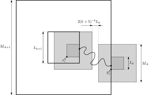
Figure 7: An illustration of the event in (7.5) and the inclusion in (7.8).

In order to employ a renormalization scheme, we will need to relate the events $A^{k}$ for different scales, as done in the following observation. Given $k\geq 1$,

$$\begin{array}[]{c}\text{there exist two collections of points $\{x^{k}_{i}\}_{i=1}^{3^{d}}$ and $\{y^{k}_{j}\}_{j=1}^{2d\cdot 7^{d-1}}$ such that}\\ \begin{array}[]{l}i)\phantom{ii)}C^{k+1}_{0}=\bigcup_{i=1}^{3^{d}}C^{k}_{x^{k}_{i}},\\ ii)\phantom{i)}\bigcup_{j=1}^{2d\cdot 7^{d-1}}C^{k}_{y^{k}_{j}}\text{ is disjoint from $D^{k+1}_{0}$ and contains $\partial(\mathbb{Z}^{d}\setminus D^{k+1}_{0})$,}\end{array}\end{array}$$ (7.7)

see Figure 7. The above statement is a consequence of (7.2) and the fact that for all $k\geq 1$ we have that $2(1+\frac{1}{(k+5)^{b}})<3$ and $6(1+\frac{1}{(k+5)^{b}})<7$. It implies that

$$A^{k+1}_{0}\subset{\textstyle\bigcup\limits_{\begin{subarray}{c}i\leq 3^{d}\\ j\leq 2d\cdot 7^{d-1}\end{subarray}}}A^{k}_{x^{k}_{i}}\cap A^{k}_{y^{k}_{j}},$$ (7.8)

see Figure 7.

It is also important to observe from (7.7) that for any $i\leq 3^{d}$ and $j\leq 2d\cdot 7^{d-1}$,

$$d\big{(}D^{k}_{x^{k}_{i}},D^{k}_{y^{k}_{j}}\big{)}\geq\lfloor L_{k+1}\rfloor-2L_{k}\overset{\eqref{e:Lkbounds}}{\geq}\frac{2^{k-1}L_{1}}{(k+5)^{b}}.$$ (7.9)

Abbreviate $\hat{u}=\frac{u^{**}+u}{2}$; since $u>u^{**}$, we have $u>\hat{u}>u^{**}$. Then, choose a sufficiently small $\varepsilon>0$ in such a way that

$$\prod_{k=1}^{\infty}\Big{(}1-\frac{\varepsilon}{k^{b}}\Big{)}>\frac{\hat{u}}{u}$$

and define

$$u_{k}=\frac{\hat{u}}{\prod_{j=1}^{k-1}(1-\varepsilon k^{-b})};$$

by construction, it holds that $u_{k}<u$ for all $k$. Abbreviate $\kappa_{d}=\frac{2d\cdot 21^{d}}{7}$ and let us denote

$$\varrho_{d}=\liminf_{L\to\infty}\mathbb{P}\big{[}[0,L]^{d}\xleftrightarrow{\mathcal{V}^{\hat{u}}}\partial[-L,2L]^{d}\big{]};$$ (7.10)

then, it holds (recall (3.6)) that $0\leq\varrho_{d}<\kappa_{d}^{-1}$. The above event stands for the fact that there exists a connecting path between these two sets through $\mathcal{V}^{\hat{u}}$.

Now, we obtain a recursive relation for $p_{k}(u_{k})$, recall (7.6).

We use (1.7) with $r=3\sqrt{d}L_{k}$, $s\geq 2^{k-1}L_{1}(k+5)^{-b}$ (recall (7.9)), $u_{k+1}$ on the place of $u$ and $\varepsilon k^{-b}$ on the place of $\varepsilon$ (observe that $u_{k}=(1-\varepsilon k^{-b})u_{k+1}$), and use also (7.3) and (7.8) to obtain that

$$p_{k+1}(u_{k+1})\leq\kappa_{d}p_{k}^{2}(u_{k})+c_{\textnormal{\tiny\ref{c:rec1}}}2^{kd}L_{1}^{d}\exp\Big{(}-c_{\textnormal{\tiny\ref{c:rec2}}}k^{-2b}\Big{(}\frac{L_{1}2^{k}}{(k+5)^{b}}\Big{)}^{d-2}\Big{)},$$ (7.11)

where $c_{\textnormal{\tiny\ref{c:rec2}}}=c_{\textnormal{\tiny\ref{c:rec2}}}(u,b,\varepsilon)$.

Now, let us first consider the case $d\geq 4$ (as mentioned above, for this case any particular value of $b\in(1,2]$ will do the job, so in the calculations below one can assume for definiteness that e.g. $b=2$). Let $h_{1}>0$ be such that $\varrho_{d}<e^{-h_{1}}<\kappa_{d}^{-1}$. Choose a sufficiently large $L_{1}\geq 100$ in such a way that $p_{1}(\hat{u})<e^{-h_{1}}$ and

$$c_{\textnormal{\tiny\ref{c:rec1}}}2^{kd}L_{1}^{d}\exp\Big{(}-c_{\textnormal{\tiny\ref{c:rec2}}}k^{-2b}\Big{(}\frac{L_{1}2^{k}}{(k+5)^{b}}\Big{)}^{d-2}+h_{1}+2^{k+1}\Big{)}<1-\kappa_{d}e^{-h_{1}}$$ (7.12)

for all $k\geq 1$ (here we used $d\geq 4$). Then, we can find small enough $h_{2}\in(0,1)$ in such a way that

$$p_{1}(\hat{u})\leq\exp(-h_{1}-2h_{2}).$$ (7.13)

We then prove by induction that

$$p_{k}(u_{k})\leq\exp(-h_{1}-h_{2}2^{k}).$$ (7.14)

Indeed, the base for the induction is provided by (7.13); then, we have by (7.11) that

$$p_{k+1}(u_{k+1})\leq\kappa_{d}\exp(-2h_{1}-h_{2}2^{k+1})+c_{\textnormal{\tiny\ref{c:rec1}}}2^{kd}L_{1}^{d}\exp\Big{(}-c_{\textnormal{\tiny\ref{c:rec2}}}k^{-2b}\Big{(}\frac{L_{1}2^{k}}{(k+5)^{b}}\Big{)}^{d-2}\Big{)}$$

so, by (7.12) (recall that $h_{2}<1$)

$$\frac{p_{k+1}(u_{k+1})}{\exp(-h_{1}-h_{2}2^{k+1})}\leq\kappa_{d}e^{-h_{1}}+c_{\textnormal{\tiny\ref{c:rec1}}}2^{kd}L_{1}^{d}\exp\Big{(}-c_{\textnormal{\tiny\ref{c:rec2}}}k^{-2b}\Big{(}\frac{L_{1}2^{k}}{(k+5)^{b}}\Big{)}^{d-2}+h_{1}+h_{2}2^{k+1}\Big{)},$$

which is smaller than one, thus proving (7.14).

Observe that for all $x$ it holds that

$$\mathbb{P}\big{[}0\xleftrightarrow{\mathcal{V}^{u}}x\big{]}\leq\mathbb{P}\big{[}[-L_{k},L_{k}]^{d}\xleftrightarrow{\mathcal{V}^{u}}\partial[-2L_{k},2L_{k}]^{d}\big{]}$$ (7.15)

with $k=\max\{m:\frac{3}{2}L_{m}<\|x\|\}$; also, $L_{k}=O(2^{k})$ by (7.3). Since $u_{k}<u$ for all $k$, (7.14) implies that $p_{k}(u)\leq\exp(-h_{1}-h_{2}2^{k})$, we obtain (3.4) from (7.15).

Let us now treat the case $d=3$. Again, let $h^{\prime}_{1}>0$ be such that $\varrho_{3}<e^{-h^{\prime}_{1}}<\kappa_{3}^{-1}$. Choose a sufficiently large $L_{1}\geq 100$ in such a way that $p_{1}(\hat{u})<e^{-h^{\prime}_{1}}$ and

$$c_{\textnormal{\tiny\ref{c:rec1}}}2^{3k}L_{1}^{3}\exp\big{(}-c_{\textnormal{\tiny\ref{c:rec2}}}(k+5)^{-3b}L_{1}2^{k-1}+h_{1}\big{)}<1-\kappa_{3}e^{-h^{\prime}_{1}}$$ (7.16)

for all $k\geq 1$. Then, we can find small enough $h^{\prime}_{2}\in\big{(}0,\frac{1}{4}c_{\textnormal{\tiny\ref{c:rec2}}}\big{)}$ in such a way that

$$p_{1}(\hat{u})\leq\exp(-h^{\prime}_{1}-2h^{\prime}_{2}).$$ (7.17)

Now, in three dimensions we are going to prove by induction that

$$p_{k}(u_{k})\leq\exp(-h^{\prime}_{1}-h^{\prime}_{2}(k+5)^{-3b}2^{k}).$$ (7.18)

Indeed, we have by (7.11) that

$$p_{k+1}(u_{k+1})\leq\kappa_{3}\exp(-2h^{\prime}_{1}-h^{\prime}_{2}(k+5)^{-3b}2^{k+1})+c_{\textnormal{\tiny\ref{c:rec1}}}2^{3k}L_{1}^{3}\exp\big{(}-c_{\textnormal{\tiny\ref{c:rec2}}}(k+5)^{-3b}L_{1}2^{k}\big{)}$$

so, by (7.16) (recall that $h_{2}<\frac{1}{4}c_{\textnormal{\tiny\ref{c:rec2}}}$)

$$\frac{p_{k+1}(u_{k+1})}{\exp(-h^{\prime}_{1}-h^{\prime}_{2}(k+6)^{-3b}2^{k+1})} \leq\kappa_{3}e^{-h^{\prime}_{1}}\exp\big{(}-h^{\prime}_{2}((k+5)^{-3b}-(k+6)^{-3b})\big{)}$$

$$\quad{}+c_{\textnormal{\tiny\ref{c:rec1}}}2^{3k}L_{1}^{3}\exp\Big{(}-c_{\textnormal{\tiny\ref{c:rec2}}}\frac{L_{1}2^{k}}{(k+5)^{3b}}+h^{\prime}_{1}+h^{\prime}_{2}\frac{2^{k+1}}{(k+6)^{3b}}\Big{)}$$

$$\leq\kappa_{3}e^{-h^{\prime}_{1}}+c_{\textnormal{\tiny\ref{c:rec1}}}2^{3k}L_{1}^{3}\exp\big{(}-c_{\textnormal{\tiny\ref{c:rec2}}}(k+5)^{-3b}L_{1}2^{k-1}+h^{\prime}_{1}\big{)}$$

$$<1,$$

thus proving (7.18). Again, since $u_{k}<u$ for all $k$, (7.14) implies that $p_{k}(u)\leq\exp(-h^{\prime}_{1}-h^{\prime}_{2}(k+5)^{-3b}2^{k})$ for all $k$, and then we obtain (3.5) with the help of (7.15) analogously to the case $d\geq 4$. This concludes the proof of Theorem 3.1. ∎

8 Smoothing of discrete sets: proof of Proposition 6.1

In this section we show that any set can be enclosed in a slightly larger set with “smooth enough” boundaries, and this larger set has the desired properties (in particular, the entrance probabilities behave in a good way), as described in Proposition 6.1.

To facilitate reading, throughout this section we will adopt the following convention for denoting points and subsets of $\mathbb{R}^{d}$ which are not (generally) in $\mathbb{Z}^{d}$: they will be respectively denoted by $\mathsf{x},\mathsf{y},\mathsf{z}$ and $\mathsf{A},\mathsf{B},\mathsf{D}$, using the sans serif font. The usual fonts are reserved to points and subsets of $\mathbb{Z}^{d}$. Also, we use the following (a bit loose but convenient) notation: if a set $\mathsf{A}\subset\mathbb{R}^{d}$ was defined, then we denote by $A\subset\mathbb{Z}^{d}$ its discretization: $A=\mathsf{A}\cap\mathbb{Z}^{d}$; conversely, if $A\subset\mathbb{Z}^{d}$ was a discrete set, then $\mathsf{A}$ just equals $A$, but is regarded as a subset of $\mathbb{R}^{d}$.

Similarly to the notations in the discrete case, let us write $\mathsf{B}(\mathsf{x},s)=\{\mathsf{y}\in\mathbb{R}^{d}:\|\mathsf{x}-\mathsf{y}\|\leq s\}$ for the balls with radius $s$, recall that $\|\cdot\|$ stands for the Euclidean norm. We abbreviate $\mathsf{B}(s)=\mathsf{B}(0,s)$. It will be convenient to define, for $\mathsf{A}\subseteq\mathbb{R}^{d}$, the ball $\mathsf{B}(\mathsf{A},s)=\bigcup_{\mathsf{x}\in\mathsf{A}}\mathsf{B}(\mathsf{x},s)$.

Definition 8.1.

Let $\mathsf{D}\subset\mathbb{R}^{d}$ be an open set (not necessarily connected) with smooth boundary $\partial\mathsf{D}$. We say that $\mathsf{D}$ is $s$-regular if for any $\mathsf{x}\in\partial\mathsf{D}$ there exist two balls $\mathsf{B}^{\mathsf{x}}_{\text{in}}\subset\bar{\mathsf{D}}$ and $\mathsf{B}^{\mathsf{x}}_{\text{out}}\subset\mathbb{R}^{d}\setminus\mathsf{D}$ of radius $s$, such that $\partial\mathsf{D}\cap\mathsf{B}^{\mathsf{x}}_{\text{out}}=\partial\mathsf{D}\cap\mathsf{B}^{\mathsf{x}}_{\text{in}}=\{\mathsf{x}\}$. Informally speaking, the above definition means that one can touch the boundary of $\mathsf{D}$ by spheres of radius $s$ from inside and outside. We also adopt the convention that $\mathbb{R}^{d}$ is $s$-regular for any $s>0$.

Observe that if $\mathsf{D}$ is an $s$-regular set , then for each $\mathsf{x}\in\partial\mathsf{D}$ the balls $\mathsf{B}^{\mathsf{x}}_{\text{in}}$ and $\mathsf{B}^{\mathsf{x}}_{\text{out}}$ are unique. Let us denote by $\mathsf{x}^{\text{in}}$ and $\mathsf{x}^{\text{out}}$ their respective centers, which lie in the line normal to $\partial\mathsf{D}$ at $\mathsf{x}$. Also, it is important to keep in mind that if $\mathsf{D}$ is $s$-regular then it is also $s^{\prime}$-regular for all $s^{\prime}\leq s$.

First, we will show that any set $\mathsf{A}\subset\mathbb{R}^{d}$ can be thickened into a smooth and regular $\mathsf{A}^{(s)}$ which is “close” to $\mathsf{A}$, see Figure 6. This is made precise in the following

Lemma 8.2.

There exists a constant $\gamma_{\textnormal{\tiny\ref{c:reg}}}\in(0,1/5)$ such that, for any set $\mathsf{A}\subset\mathbb{R}^{d}$ and $s>0$, there exist a set $\mathsf{A}^{(s)}\subset\mathbb{R}^{d}$ with smooth boundary, such that

1. $\mathsf{A}\subseteq\mathsf{A}^{(s)}\subseteq\mathsf{B}\big{(}\mathsf{A},\frac{s}{5}\big{)}$ and

2. $\mathsf{A}^{(s)}$ is $\gamma_{\textnormal{\tiny\ref{c:reg}}}s$-regular in the sense of Definition 8.1.

Proof.

Assume that $\mathbb{R}^{d}\setminus\mathsf{B}\big{(}\mathsf{A},\frac{s}{5}\big{)}$ is nonempty, otherwise the claim is straightforward. Since we suppose that $\mathsf{A}\subset\mathbb{R}^{d}$ is arbitrary, we can suppose that $s=5$ (so that $\frac{s}{5}$=1) by scaling $\mathsf{A}$ if necessary.

Let us first tile the space $\mathbb{R}^{d}$ with compact cubes $\mathsf{K}_{m}$, of side length $\frac{1}{8\sqrt{d}}$. More precisely, for $m=(m_{1},\dots,m_{d})\in\mathbb{Z}^{d}$, let

$$\mathsf{K}_{m}=\tfrac{1}{8\sqrt{d}}[m_{1},m_{1}+1]\times\dots\times[m_{d},m_{d}+1].$$ (8.1)

With the above definition, $\operatorname{diam}(\mathsf{K}_{m_{1}}\cup\mathsf{K}_{m_{2}})\leq\frac{1}{4}$ if $\mathsf{K}_{m_{1}}$ and $\mathsf{K}_{m_{2}}$ have at least one common point.

We first consider the set

$$\hat{\mathsf{A}}=\bigcup\mathsf{K}_{m},$$

where the above union is taken over all cubes that either intersect $\mathsf{A}$ or have at least one common point with another cube that intersects $\mathsf{A}$.

Define now the function $\hat{f}$ to be the convolution of ${{1}}_{\hat{\mathsf{A}}}(\cdot)$ with a smooth test function $\psi\geq 0$, with $\int\psi\,d\mathsf{x}=1$ and supported on $\mathsf{B}(\frac{1}{8})$. Clearly, for any $\alpha\in(0,1)$ it holds that

$$\mathsf{A}\subseteq\{\mathsf{x}:\hat{f}(\mathsf{x})>\alpha\},$$ (8.2)

so it remains to show that, for some $\alpha$, the set $\{\mathsf{x}:\hat{f}(\mathsf{x})>\alpha\}$ is $\gamma_{\textnormal{\tiny\ref{c:reg}}}$-regular for some small enough $\gamma_{\textnormal{\tiny\ref{c:reg}}}<\frac{1}{5}$ independent of $\mathsf{A}$.

To understand how the above construction depends on the choice of $\mathsf{A}$, let us scale and recenter the function $\hat{f}$. More precisely, let $\varphi_{\mathsf{A},m}:\mathsf{B}(0,1)\to\mathbb{R}_{+}$ be the function that associates a point $\mathsf{x}\in\mathsf{B}(0,1)$ to $\hat{f}(\mathsf{x}-m)$. It is important to observe that

$$\begin{array}[]{c}\text{as we vary $\mathsf{A}\subset\mathbb{Z}^{d}$, and $m\in\mathbb{Z}^{d}$, the functions}\\ \text{$\varphi_{\mathsf{A},m}$ range over a finite collection of smooth functions,}\end{array}$$ (8.3)

since it is determined by the finitely many possible configurations of boxes $K_{m^{\prime}}$ that intersect $\mathsf{K}_{m}$ (whether they appear or not in the union defining $\hat{\mathsf{A}}$).

From the Sard’s theorem and the implicit function theorem one can obtain that for some $\alpha\in(0,1)$ (in fact, for generic values of $\alpha\in(0,1)$) the boundary $\{\mathsf{x}:\hat{f}(\mathsf{x})=\alpha\}$ is smooth. Therefore, using (8.3) we can choose $\alpha_{o}\in(0,1)$ such that $\{\mathsf{x}:\hat{f}(\mathsf{x})=\alpha_{o}\}$ is smooth, independently of the choice of $\mathsf{A}$. We now let $\mathsf{A}^{\prime}=\{\mathsf{x}:\hat{f}(\mathsf{x})>\alpha_{o}\}$. From (8.2), we conclude that $\mathsf{A}\subset\mathsf{A}^{\prime}$ and from the definition of $\hat{f}$, we obtain that $\mathsf{A}^{\prime}\subseteq\mathsf{B}(\mathsf{A},1)$. To finish the proof, we should show that $\mathsf{A}^{\prime}$ is $\gamma_{\textnormal{\tiny\ref{c:reg}}}$-regular (with some small enough constant $\gamma_{\textnormal{\tiny\ref{c:reg}}}$ independent of $\mathsf{A}$).

Since $\partial\mathsf{A}^{\prime}$ is smooth, we can show that for every $\mathsf{x}\in\partial\mathsf{A}^{\prime}$, there exist $\mathsf{B}_{\text{in}}$ and $\mathsf{B}_{\text{out}}$ as in Definition 8.1. Observe that the existence of such balls with radius smaller or equal to $1/4$ only depends on the values of $\hat{f}$ in $\mathsf{B}(\mathsf{x},1)$. So that the independence of $\gamma_{\textnormal{\tiny\ref{c:reg}}}$ of the choice of $\mathsf{A}$ follows from (8.3). ∎

At this point, we can collect the first ingredient for Proposition 6.1: we take $A^{(s)}$ to be the discretization of the set $\mathsf{A}^{(s)}$ provided by Lemma 8.2.

Now, we prove several geometric properties of regular sets and their discretizations.

Lemma 8.3.

Abbreviate $\gamma_{\textnormal{\tiny\ref{g:til}}}=\frac{1}{200}$ and $\gamma_{\textnormal{\tiny\ref{g:1/6}}}=\frac{1+\sqrt{799}}{200}<\frac{1}{6}$. Then for any $s$-regular set $\mathsf{A}$ and for any $\mathsf{v}_{1},\mathsf{v}_{2}\in\partial\mathsf{A}$ such that $\|\mathsf{v}_{1}-\mathsf{v}_{2}\|\leq\gamma_{\textnormal{\tiny\ref{g:til}}}s$ it holds that

$$\|\mathsf{v}_{1}^{\text{\rm out}}-\mathsf{v}_{2}^{\text{\rm out}}\|\leq\gamma_{\textnormal{\tiny\ref{g:1/6}}}s$$ (8.4)

(observe that, by symmetry, the same holds for $\mathsf{v}_{1}^{\text{\rm in}},\mathsf{v}_{2}^{\text{\rm in}}$).

Proof.

Consider the plane $\mathcal{L}$ generated by points $\mathsf{v}_{1}$, $\mathsf{v}_{1}^{\text{\rm out}}$, and $\mathsf{v}_{2}^{\text{\rm out}}+(\mathsf{v}_{1}-\mathsf{v}_{2})$, see Figure 8 (note that, as indicated on the picture, $\mathsf{v}_{2}$ need not lie on this plane).

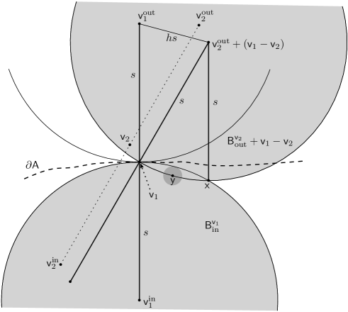
Figure 8: Depiction of the plane $\mathcal{L}$ on the proof of Lemma 8.3. The radius of the small gray circle centered in $\mathsf{y}$ is $as$; also, on this picture the segment between $\mathsf{v}_{2}^{\text{\rm in}}$ and $\mathsf{v}_{2}^{\text{\rm out}}$ (containing also $\mathsf{v}_{2}$) does not have an intersection with the plane $\mathcal{L}$. That is why $v_{2}$ appears not to intersect $\partial A$.

Let $\mathsf{x}$ be the point that lies on the intersection of $\partial\mathsf{B}^{\mathsf{v}_{1}}_{\text{in}}\cap(\partial\mathsf{B}^{\mathsf{v}_{2}}_{\text{out}}+{\mathsf{v}_{1}}-{\mathsf{v}_{2}})$ with $\mathcal{L}$ and is different from $\mathsf{v}_{1}$, and let $\mathsf{y}$ be the middle point on the arc of the circle $(\partial\mathsf{B}^{\mathsf{v}_{2}}_{\text{out}}+{\mathsf{v}_{1}}-{\mathsf{v}_{2}})\cap\mathcal{L}$ between $\mathsf{v}_{1}$ and $\mathsf{x}$ (of course, we mean the arc that lies inside $\mathsf{B}^{\mathsf{v}_{1}}_{\text{in}}$). Abbreviate also $h=s^{-1}\|\mathsf{v}_{2}^{\text{\rm out}}+(\mathsf{v}_{1}-\mathsf{v}_{2})-\mathsf{v}_{1}^{\text{\rm out}}\|$ and $a=s^{-1}d(\mathsf{y},\partial\mathsf{B}^{\mathsf{v}_{1}}_{\text{in}})$; with some elementary geometry, we obtain that

$$h=2\sqrt{a-\frac{a^{2}}{4}}.$$

But, we must necessarily have

$$d(\mathsf{y},\partial\mathsf{B}^{\mathsf{v}_{1}}_{\text{in}})\leq\|\mathsf{v}_{1}-\mathsf{v}_{2}\|,$$

because otherwise the point $\mathsf{y}-\mathsf{v}_{1}+\mathsf{v}_{2}\in\mathsf{B}^{\mathsf{v}_{2}}_{\text{out}}$ would also belong to the interior of $\mathsf{B}^{\mathsf{v}_{1}}_{\text{in}}$, a contradiction. So, we have

$$h\leq 2\sqrt{\gamma_{\textnormal{\tiny\ref{g:til}}}-\frac{\gamma_{\textnormal{\tiny\ref{g:til}}}^{2}}{4}}=\frac{\sqrt{799}}{200},$$

which means that

$$\|\mathsf{v}_{1}^{\text{\rm out}}-\mathsf{v}_{2}^{\text{\rm out}}\|<\Big{(}\frac{\sqrt{799}}{200}+\gamma_{\textnormal{\tiny\ref{g:til}}}\Big{)}s=\gamma_{\textnormal{\tiny\ref{g:1/6}}}s.$$

∎

The next lemma is a consequence of an obvious observation that the boundary of discretized $s$-regular sets looks locally flat for large $s$:

Lemma 8.4.

There exist (large enough) $s_{0},h_{0}$ with the following properties. Assume that $\mathsf{A}$ is $s$-regular for some $s\geq s_{0}$ and $x,y\notin A$ are such that $\|x-y\|\leq 3\sqrt{d}$. Then there exists a path between $x$ and $y$ of length at most $h_{0}$ that does not intersect $A$.

Proof.

This result is fairly obvious, so we give only a sketch of the proof (certainly, not the most “economic” one). First, without restricting generality, one can assume that $\max(d(x,\mathsf{A}),d(y,\mathsf{A}))<3\sqrt{d}$ (otherwise, the ball of radius $3\sqrt{d}$ centered in one of the points does not have intersection with $A$ and contains the other point; then, use the fact that this discrete ball is a connected graph). Then, let $\mathsf{z}\in\partial\mathsf{A}$ be a point on the boundary closest to $x$, $z$ be the point in $A$ closest to $\mathsf{z}$, and consider the cube

$$G=\{z^{\prime}\in\mathbb{Z}^{d}:\|z^{\prime}-z\|_{\infty}\leq\lceil 7\sqrt{d}\rceil\}$$

(where $\|\cdot\|_{\infty}$ is the maximum norm). Assume without loss of generality that the projection of the normal vector to $\partial\mathsf{A}$ at $\mathsf{z}$ on the first coordinate vector is at least $\frac{1}{\sqrt{d}}$. Then, the claim of the lemma follows once we prove that for all large enough $s$

the set $$G\setminus\mathsf{A}$$ is connected. (8.5)

Indeed, for $s$ large enough $\{v,v+e_{1}\}$ is not fully inside $\mathbb{R}^{d}\setminus(\mathsf{B}_{\text{in}}^{\mathsf{z}}\cup\mathsf{B}_{\text{out}}^{\mathsf{z}})$ for any $v$ in $G$. This implies that $G\setminus\mathsf{A}$ is given by $G\cap\mathsf{B}^{z}_{\text{out}}$ together with some extra points in the neighborhood of this set, implying (8.5) and concluding the proof of the lemma. ∎

Observe that Lemma 8.4 implies that for any $x\in\partial A$ and $y\notin A$ such that $\|x-y\|\leq 2\sqrt{d}$, it holds that

$$P_{y}[X_{H_{A}}=x]\geq(2d)^{-h_{0}}.$$ (8.6)

Next, we need an elementary result about escape probabilities from spheres:

Lemma 8.5.

There exist positive constants $s_{1},c_{\textnormal{\tiny\ref{c:L34''}}},c_{\textnormal{\tiny\ref{c:L34'''}}},c_{\textnormal{\tiny\ref{c:LL34''}}},c_{\textnormal{\tiny\ref{c:LL34'''}}}$ (depending only on the dimension) such that for all $\mathsf{y}\in\mathbb{R}^{d}$, for all $s\geq s_{1}$ and every $x\in B(\mathsf{y},2s)\setminus B(\mathsf{y},s)$, we have

$$c_{\textnormal{\tiny\ref{c:L34''}}}\frac{\|x-\mathsf{y}\|-s}{s}\leq P_{x}[H_{B(\mathsf{y},s)}>H_{\mathbb{Z}^{d}\setminus B(\mathsf{y},2s)}]\leq c_{\textnormal{\tiny\ref{c:L34'''}}}\frac{\|x-\mathsf{y}\|-s+1}{s},$$ (8.7)

and for all $x\in B(\mathsf{y},3s)\setminus B(\mathsf{y},s)$

$$c_{\textnormal{\tiny\ref{c:LL34''}}}\frac{3s-\|x-\mathsf{y}\|}{s}\leq P_{x}[H_{B(\mathsf{y},s)}<H_{\mathbb{Z}^{d}\setminus B(\mathsf{y},3s)}]\leq c_{\textnormal{\tiny\ref{c:LL34'''}}}\frac{3s-\|x-\mathsf{y}\|+1}{s}.$$ (8.8)

Proof.

By a direct calculation, it is elementary to obtain that, for large enough $s$ (not depending on $\mathsf{y}$), the process $\|X_{n\wedge H_{B(s)}}-\mathsf{y}\|^{-(d-1)}$ is a supermartingale, and $\|X_{n\wedge H_{B(s)}}-\mathsf{y}\|^{-(d-\tfrac{5}{2})}$ is a submartingale, see e.g. the proof of Lemma 1 in [5]. From the Optional Stopping Theorem, we obtain that

$$\frac{s^{-(d-1)}-\|x-\mathsf{y}\|^{-(d-1)}}{s^{-(d-1)}-(2s+1)^{-(d-1)}}\leq P_{x}[H_{B(s)}>H_{\mathbb{Z}^{d}\setminus B(2s)}]\leq\frac{(s-1)^{-d+\tfrac{5}{2}}-\|x-\mathsf{y}\|^{-d+\tfrac{5}{2}}}{(s-1)^{-d+\tfrac{5}{2}}-(2s)^{-d+\tfrac{5}{2}}},$$ (8.9)

where the above balls are centered in $\mathsf{y}$. Then (8.7) follows from (8.9) with the observation that $0<\frac{\|x-\mathsf{y}\|}{s}\leq 2$ and some elementary calculus. The proof of (8.8) is completely analogous.

In fact, with some more effort, one can obtain that $s_{1}=\frac{\sqrt{d}}{2}$ (observe that $B(\mathsf{y},\frac{\sqrt{d}}{2})$ is nonempty for all $\mathsf{y}\in\mathbb{R}^{d}$), but we do not need this stronger fact for the present paper. ∎

We now need estimates on the entrance measure of a set in $\mathbb{Z}^{d}$ which has been obtained from the discretization of a regular set $\mathsf{D}\subset\mathbb{R}^{d}$. For this, we will need the following definitions. Let $D=\mathsf{D}\cap\mathbb{Z}^{d}$ and fix $x\in\partial D$, we write $\mathsf{x}$ for the closest point to $x$ in $\partial\mathsf{D}$ (it can be chosen arbitrarily in case of ties) and note that $\lVert x-\mathsf{x}\rVert\leq 1$. We define $x^{\text{in}}$ and $x^{\text{out}}$ to be the closest points to $\mathsf{x}^{\text{in}}$ and $\mathsf{x}^{\text{out}}$ in $\mathbb{Z}^{d}$ (again chosen arbitrarily in case of ties). Observe that $\lVert x^{\text{out}}-\mathsf{x}^{\text{out}}\rVert$ is at most $\frac{\sqrt{d}}{2}$ (and the same holds for $x^{\text{in}}$ and $\mathsf{x}^{\text{in}}$).

Lemma 8.6.

• Suppose that $\mathsf{A}$ is an $s$-regular set for some $s\geq s_{0}+\sqrt{d}$ and $y\in\partial A,x\in\mathbb{Z}^{d}\setminus A$ are such that $\|x-y\|\geq 2s$. Then $P_{x}[X_{H_{A}}=y]\leq c_{\textnormal{\tiny\ref{c:L35''}}}s^{-(d-1)}$.

• Assume that $\mathsf{A}$ is $s$-regular with $s\geq s_{0}+\sqrt{d}$ and $y\in\partial A$; then for every $x\in B(y^{out},s/2)$, we have $P_{x}[X_{H_{A}}=y,H_{A}<H_{\mathbb{Z}^{d}\setminus B(y^{out},s+\sqrt{d})}]\geq c_{\textnormal{\tiny\ref{c:L35'''}}}s^{-(d-1)}$.

Proof.

Given $\mathsf{A}$ and $y\in\partial A$ as above, recall that $\mathsf{y}$ stands for the closest point to $y$ in $\partial\mathsf{A}$ (chosen arbitrarily in case of ties). By Definition 8.1, we know that the ball $\mathsf{B}^{\mathsf{y}}_{\text{in}}\subset\mathbb{R}^{d}$ of radius $s$ lies fully inside $\mathsf{A}$. Moreover, since $y^{\text{in}}$ is at distance at most $\frac{\sqrt{d}}{2}$ from $\mathsf{y}^{\text{in}}$, we conclude that

$$B^{y}_{\text{in}}:=B\Big{(}y^{\text{in}},s-\frac{\sqrt{d}}{2}\Big{)}\subseteq\mathsf{B}^{\mathsf{y}}_{\text{in}},\text{ and also }B^{y}_{\text{out}}:=B\Big{(}y^{\text{out}},s-\frac{\sqrt{d}}{2}\Big{)}\subseteq\mathsf{B}^{\mathsf{y}}_{\text{out}},$$ (8.10)

see Figure 9.

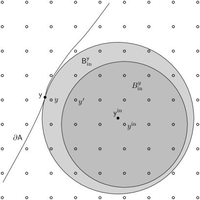
Figure 9: On the proof of Lemma 8.6

Let $y^{\prime}\in\partial B^{y}_{\text{in}}$ be the point which is closest to $y$ (it could happen that $y^{\prime}$ is $y$ itself). By construction we have $d(y,B^{y}_{\text{in}})\leq\sqrt{d}$, therefore $\|y-y^{\prime}\|\leq\frac{3}{2}\sqrt{d}$, and so by Lemma 8.4 we have

$$P_{x}[X_{H_{B}}=y^{\prime}]\geq c_{\textnormal{\tiny\ref{c:yyprime}}}P_{x}[X_{H_{A}}=y].$$ (8.11)

Employing Proposition 6.5.4 of [10], we obtain that

$$P_{x}[X_{H_{B}}=y^{\prime}]\leq c_{\textnormal{\tiny\ref{c:L35''}}}s^{-(d-1)},$$ (8.12)

which together with (8.11) proves (i).

A discretization argument analogous to the above gives (ii) for all $x\in B(y^{out},\frac{s}{2}-\frac{\sqrt{d}}{4})$ as a direct consequence of Lemma 6.3.7 of [10]; then, using Lemma 8.4, we obtain the desired statement for all $x\in B(y^{out},\frac{s}{2})$. ∎

Next, aiming to the proof of (6.5), we formulate and prove the following result:

Proposition 8.7.

There exist constants $s_{0},\gamma_{\textnormal{\tiny\ref{reg8}}},\gamma_{\textnormal{\tiny\ref{reg10}}}>0$ such that if $s\geq s_{0}$, $\mathsf{A}\subset\mathbb{R}^{d}$ is $\gamma_{\textnormal{\tiny\ref{c:reg}}}s$-regular and if $y_{1},y_{2}\in\partial A$ are such that $\|y_{1}-y_{2}\|\leq\gamma_{\textnormal{\tiny\ref{reg8}}}s$, then there exists a set $\hat{D}$ (depending on $y_{1},y_{2}$) that separates $\{y_{1},y_{2}\}$ from $\partial B(y_{1},2\gamma_{\textnormal{\tiny\ref{c:reg}}}s)$ (i.e., any nearest-neighbor path starting at $\partial B(y_{1},2\gamma_{\textnormal{\tiny\ref{c:reg}}}s)$ that enters $A$ at $\{y_{1},y_{2}\}$, must pass through $\hat{D}$) such that

$$\sup_{\begin{subarray}{c}x\in\hat{D};\\ P_{x}[X_{H_{A}}=y_{1}]>0\end{subarray}}\frac{P_{x}[X_{H_{A}}=y_{2}]}{P_{x}[X_{H_{A}}=y_{1},H_{A}<H_{\mathbb{Z}^{d}\setminus B(y_{1},\frac{5}{2}\gamma_{\textnormal{\tiny\ref{c:reg}}}s)}]}\leq\gamma_{\textnormal{\tiny\ref{reg10}}}.$$ (8.13)

Let us already mention that the constants $\gamma_{\textnormal{\tiny\ref{reg8}}},\gamma_{\textnormal{\tiny\ref{reg10}}}$ here are exactly those that we need in Proposition 6.1.

Proof of Proposition 8.7.

Define

$$s_{2}=\max\big{\{}\gamma_{\textnormal{\tiny\ref{c:reg}}}^{-1}s_{0},\;36(\gamma_{\textnormal{\tiny\ref{c:reg}}}\gamma_{\textnormal{\tiny\ref{g:til}}})^{-1}(s_{1}+\sqrt{d})\big{\}}\geq 18(\gamma_{\textnormal{\tiny\ref{c:reg}}}\gamma_{\textnormal{\tiny\ref{g:til}}})^{-1}.$$ (8.14)

Also, we define $\gamma_{\textnormal{\tiny\ref{reg8}}}=\frac{1}{3}\gamma_{\textnormal{\tiny\ref{c:reg}}}\gamma_{\textnormal{\tiny\ref{g:til}}}$. Given $y_{1}$ and $y_{2}$ in $\partial A$ such that $\|y_{1}-y_{2}\|<\gamma_{\textnormal{\tiny\ref{reg8}}}s$, let us define

$$D=\Big{\{}z\in\mathbb{Z}^{d}\setminus A:d(z,\mathsf{A})\leq\frac{1}{2}\gamma_{\textnormal{\tiny\ref{reg8}}}s\text{ and }d(z,y_{k})\leq 2\gamma_{\textnormal{\tiny\ref{reg8}}}s,k=1,2\Big{\}},$$ (8.15)

and

$$\hat{D}=\big{\{}z\in D:\text{ there exists }v\in\mathbb{Z}^{d}\setminus(A\cup D)\text{ such that $z$ and $v$ are neighbors}\big{\}},$$ (8.16)

see Figure 10. Intuitively speaking, $\hat{D}$ is the part of the boundary of $D$ not adjacent to $A$.

We now claim that

$$\begin{array}[]{c}\text{all sites of~{}$\hat{D}$ are at distance at least $\displaystyle\frac{1}{2}\gamma_{\textnormal{\tiny\ref{reg8}}}s-1$ from $\{y_{1},y_{2}\}$.}\end{array}$$ (8.17)

To see why this is true, observe first that for $z\in\hat{D}$, the point $v\leftrightarrow z$ as in (8.16) is not in $D$. Therefore, we either have $d(v,\{y_{1},y_{2}\})>2\gamma_{\textnormal{\tiny\ref{reg8}}}s$ or $d(v,\mathsf{A})\geq\frac{1}{2}\gamma_{\textnormal{\tiny\ref{reg8}}}s$, in both cases (8.17) holds.

In fact, to prove (8.13), it is enough to prove that for all $z\in\hat{D}$

$$P_{x}[X_{H_{A}}=y_{1},H_{A}<H_{\mathbb{Z}^{d}\setminus B(y_{1},\frac{5}{2}\gamma_{\textnormal{\tiny\ref{c:reg}}}s)}]\geq c_{\textnormal{\tiny\ref{c:hitfrom_z'}}}\frac{d(z,A)}{s^{d}}$$ (8.18)

and

$$P_{z}[X_{H_{A}}=y_{2}]\leq c_{\textnormal{\tiny\ref{c:hitfrom_z''}}}\frac{d(z,A)}{s^{d}}.$$ (8.19)

The idea behind these two bounds is depicted on Figure 10, which we now turn into a rigorous proof.

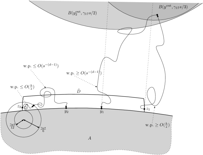
Figure 10: On the proof of Proposition 8.7: lower bound for $P_{z_{1}}[X_{H_{A}}=y_{1},\dots]$ and upper bound for $P_{z_{2}}[X_{H_{A}}=y_{2}]$; we have $h\simeq d(z_{1,2},A)$, and “w.p.” stands for “with probability”.

To obtain (8.18), we proceed in the following way. Consider some $\mathsf{y}\in\partial A$ such that $d(z,A)\geq\|z-\mathsf{y}\|$, and observe that (8.8) implies that

$$P_{z}[H_{B(\mathsf{y}^{\text{out}},\gamma_{\textnormal{\tiny\ref{c:reg}}}s/3)}<H_{A}]\geq\frac{c_{\textnormal{\tiny\ref{c:dist/s}}}d(z,A)}{s}.$$ (8.20)

Let $\mathsf{y}_{k}\in\partial A$ be the closest boundary point to $y_{k}$; clearly, we have $\|\mathsf{y}_{k}-y_{k}\|\leq 1$. Then, it holds that $\|y_{1}-z\|\leq 2\gamma_{\textnormal{\tiny\ref{reg8}}}s$ and $\|z-\mathsf{y}\|\leq\frac{1}{2}\gamma_{\textnormal{\tiny\ref{reg8}}}s$, and thus, by (8.14)

$$\|\mathsf{y}_{1}-\mathsf{y}\|\leq\frac{5}{2}\gamma_{\textnormal{\tiny\ref{reg8}}}s+1<3\gamma_{\textnormal{\tiny\ref{reg8}}}s=\gamma_{\textnormal{\tiny\ref{c:reg}}}\gamma_{\textnormal{\tiny\ref{g:til}}}s.$$

So, by Lemma 8.3 it holds that $\|\mathsf{y}^{\text{out}}-\mathsf{y}_{1}^{\text{out}}\|\leq\gamma_{\textnormal{\tiny\ref{c:reg}}}\gamma_{\textnormal{\tiny\ref{g:1/6}}}s<\frac{1}{6}\gamma_{\textnormal{\tiny\ref{c:reg}}}s$, which implies that $\mathsf{B}(\mathsf{y}^{\text{out}},\frac{1}{3}\gamma_{\textnormal{\tiny\ref{c:reg}}}s)\subset\mathsf{B}(\mathsf{y}_{1}^{\text{out}},\frac{1}{2}\gamma_{\textnormal{\tiny\ref{c:reg}}}s)$. Observing that $B(y_{1}^{\text{out}},\gamma_{\textnormal{\tiny\ref{c:reg}}}s+\sqrt{d})\subset B(y_{1},\frac{5}{2}\gamma_{\textnormal{\tiny\ref{c:reg}}}s)$ Applying Lemma 8.6 (ii) and using (8.20), we obtain (8.18).

To prove (8.19), we proceed in the following way. Recall that if a set is $r$-regular then it is $r^{\prime}$-regular for all $r^{\prime}\leq r$; so, if $d(z,A)\geq\frac{1}{3}\gamma_{\textnormal{\tiny\ref{reg8}}}s$ then Lemma 8.6 (i) already implies (8.19). Assume now that $z\in\hat{D}$ is such that $d(z,A)<\frac{1}{3}\gamma_{\textnormal{\tiny\ref{reg8}}}s$ and let $\mathsf{y}\in\partial\mathsf{A}$ be such that $d(z,A)\geq\|z-\mathsf{y}\|$. Let us show that then we have $\|\mathsf{y}-y_{2}\|\geq\frac{1}{2}\gamma_{\textnormal{\tiny\ref{reg8}}}s$. Indeed, by construction of $\hat{D}$ there exists $v\notin A\cup G$ with $\|z-v\|=1$ and such that either $d(v,A)\geq\frac{1}{2}\gamma_{\textnormal{\tiny\ref{reg8}}}s$ or $\min(\|v-y_{1}\|,\|v-y_{2}\|)>2\gamma_{\textnormal{\tiny\ref{reg8}}}s$. The first possibility is ruled out since then we would have $d(z,A)>\frac{1}{2}\gamma_{\textnormal{\tiny\ref{reg8}}}s-1$ which contradicts to $d(z,A)<\frac{1}{3}\gamma_{\textnormal{\tiny\ref{reg8}}}s$ because of (8.14). Then, the second alternative implies that $\|v-y_{2}\|>\gamma_{\textnormal{\tiny\ref{reg8}}}s$, so $\|z-y_{2}\|>\gamma_{\textnormal{\tiny\ref{reg8}}}s-1$. This means that

$$\|\mathsf{y}-y_{2}\|\geq\gamma_{\textnormal{\tiny\ref{reg8}}}s-1-\frac{1}{3}\gamma_{\textnormal{\tiny\ref{reg8}}}s\geq\frac{1}{2}\gamma_{\textnormal{\tiny\ref{reg8}}}s$$

again because of (8.14).

Let $\hat{\mathsf{v}}$ be the center of the ball with radius $\frac{1}{12}\gamma_{\textnormal{\tiny\ref{reg8}}}s$ that touches $\partial\mathsf{A}$ at $\mathsf{y}$ from inside; we have by (8.14) that

$$\inf_{v^{\prime}\in\mathsf{B}(\hat{\mathsf{v}},\frac{1}{6}\gamma_{\textnormal{\tiny\ref{reg8}}}s)}\|v^{\prime}-y_{2}\|\geq\frac{1}{2}\gamma_{\textnormal{\tiny\ref{reg8}}}s-\frac{1}{4}\gamma_{\textnormal{\tiny\ref{reg8}}}s-1\geq\frac{1}{12}\gamma_{\textnormal{\tiny\ref{reg8}}}s+1.$$

Then, one can write

$$P_{z}[X_{H_{A}}=y_{2}]\leq P_{z}[H_{\mathbb{Z}^{d}\setminus B(\hat{\mathsf{v}},\frac{1}{6}\gamma_{\textnormal{\tiny\ref{reg8}}}s)}<H_{B(\hat{\mathsf{v}},\frac{1}{12}\gamma_{\textnormal{\tiny\ref{reg8}}}s)}]\sup_{z^{\prime}:\|z^{\prime}-y_{2}\|\geq\frac{1}{12}\gamma_{\textnormal{\tiny\ref{reg8}}}s}P_{z^{\prime}}[X_{H_{A}}=y_{2}],$$

and use Lemma 8.5 to obtain that the first term in the right-hand side of the above display is at most $c_{\textnormal{\tiny\ref{c:endproof'}}}s^{-1}d(z,A)$. By Lemma 8.6 (i), the second term is bounded from above by $c_{\textnormal{\tiny\ref{c:endproof''}}}s^{-(d-1)}$. This concludes the proof of (8.19) and hence of Proposition 8.7. ∎

We now collect the ingredients necessary for the proof of Proposition 6.1:

• as already mentioned just before Lemma 8.3, the sets $A^{(s)}_{1,2}$ are the discretizations of the sets $\mathsf{A}^{(s)}_{1,2}$ provided by Lemma 8.2;

• we take the same $s_{2}$ provided by (8.14) and define $\gamma_{\textnormal{\tiny\ref{regular}}}=\frac{1}{2}\gamma_{\textnormal{\tiny\ref{c:reg}}}$;

• existence of $\gamma_{\textnormal{\tiny\ref{reg2}}}$ suitable for (6.2) and (6.3) follows then from Lemma 8.6;

• the claim (6.5) follows from Proposition 8.7, with the right constants $\gamma_{\textnormal{\tiny\ref{reg8}}},\gamma_{\textnormal{\tiny\ref{reg10}}}$, as we already mentioned.

So, the only unattended item in Proposition 6.1 is (6.4). But it is straightforward to obtain (6.4) from a projection argument: let $\mathsf{y}\in\partial\mathsf{A}_{k}^{(s)}$ be a closest point to $y\in\partial A_{k}^{(s)}$ and assume without lost of generality that the projection of the normal vector at $\mathsf{y}$ to the first coordinate is at least $\frac{1}{\sqrt{d}}$. Then, the intersection of projections of $\mathsf{B}^{\mathsf{y}}_{\text{in}}\cap\mathsf{B}(\mathsf{y},\gamma_{\textnormal{\tiny\ref{reg8}}}s-1)$ and $\mathsf{B}^{\mathsf{y}}_{\text{out}}\cap\mathsf{B}(\mathsf{y},\gamma_{\textnormal{\tiny\ref{reg8}}}s-1)$ along the first coordinate axis contains a ($(d-1)$-dimensional) ball of radius $O(s)$, and this proves (6.4) (since on the preimage of each integer point which lies within this intersection there should be at least one point of $\partial A_{k}^{(s)}\cap B(y,\gamma_{\textnormal{\tiny\ref{reg8}}}s)$). This concludes the proof of Proposition 6.1. $\Box$

Acknowledgments. The authors are very grateful to Caio Alves, Pierre-François Rodriguez and the anonymous referee, who carefully read the manuscript, making many useful suggestions and corrections. S.P. was partially supported by FAPESP (grant 2009/52379–8) and CNPq (grant 300886/2008–0). A.T. received support from CNPq (grant 306348/2012–3). The authors thank IMPA and IMECC–UNICAMP for financial support and hospitality during their mutual visits.

References

- [1] David Belius. Cover levels and random interlacements. Ann. Appl. Probab., 22(2):522–540, 2012.
- [2] David Belius. Gumbel fluctuations for cover times in the discrete torus. Probab. Theory Relat. Fields, 157(3-4):635–689, 2013.
- [3] Jiří Černý, Augusto Teixeira, and David Windisch. Giant vacant component left by a random walk in a random -regular graph. Ann. Inst. Henri Poincaré Probab. Stat., 47(4):929–968, 2011.
- [4] Jiří Černý and Serguei Popov. On the internal distance in the interlacement set. Electron. J. Probab., 17:no. 29, 1–25, 2012.
- [5] F. den Hollander, M.V. Menshikov, and S.Yu. Popov. A note on transience versus recurrence for a branching random walk in random environment. J. Statist. Phys., 95(3-4):587–614, 1999.
- [6] Alexander Drewitz, Balázs Ráth, and Artëm Sapozhnikov. Local percolative properties of the vacant set of random interlacements with small intensity. Ann. Inst. Henri Poincaré, Probab. Stat., 50(4):1165–1197, 2014.
- [7] P. J. Fitzsimmons and Jim Pitman. Kac’s moment formula and the Feynman-Kac formula for additive functionals of a Markov process. Stochastic Process. Appl., 79(1):117–134, 1999.
- [8] Geoffrey Grimmett. Percolation, volume 321 of Grundlehren der Mathematischen Wissenschaften [Fundamental Principles of Mathematical Sciences]. Springer-Verlag, Berlin, second edition, 1999.
- [9] Gregory F. Lawler. Intersections of random walks. Probability and its Applications. Birkhäuser Boston Inc., Boston, MA, 1991.
- [10] Gregory F. Lawler and Vlada Limic. Random walk: a modern introduction, volume 123 of Cambridge Studies in Advanced Mathematics. Cambridge University Press, Cambridge, 2010.
- [11] M. V. Men′shikov. Coincidence of critical points in percolation problems. Dokl. Akad. Nauk SSSR, 288(6):1308–1311, 1986.
- [12] Mikhail Menshikov and Serguei Popov. On range and local time of many-dimensional submartingales. J. Theor. Probab., 27(2):601–617, 2014.
- [13] Yuval Peres, Alistair Sinclair, Perla Sousi, and Alexandre Stauffer. Mobile geometric graphs: detection, coverage and percolation. In Proceedings of the Twenty-Second Annual ACM-SIAM Symposium on Discrete Algorithms, pages 412–428, Philadelphia, PA, 2011. SIAM.
- [14] Balázs Ráth and Artëm Sapozhnikov. On the transience of random interlacements. Electron. Commun. Probab., 16:379–391, 2011.
- [15] Balázs Ráth and Artëm Sapozhnikov. The effect of small quenched noise on connectivity properties of random interlacements. Electron. J. Probab., 18:20, 2013.
- [16] Sidney I. Resnick. Extreme values, regular variation and point processes. Springer Series in Operations Research and Financial Engineering. Springer, New York, 2008. Reprint of the 1987 original.
- [17] Yu. A. Rozanov. Markov random fields. Applications of Mathematics. Springer-Verlag, New York, 1982. Translated from Russian by Constance M. Elson.
- [18] Vladas Sidoravicius and Alain-Sol Sznitman. Percolation for the vacant set of random interlacements. Comm. Pure Appl. Math., 62(6):831–858, 2009.
- [19] Vladas Sidoravicius and Alain-Sol Sznitman. Connectivity bounds for the vacant set of random interlacements. Ann. Inst. Henri Poincaré Probab. Stat., 46(4):976–990, 2010.
- [20] Alain-Sol Sznitman. On the domination of random walk on a discrete cylinder by random interlacements. Electron. J. Probab., 14:no. 56, 1670–1704, 2009.
- [21] Alain-Sol Sznitman. Random walks on discrete cylinders and random interlacements. Probab. Theory Related Fields, 145(1-2):143–174, 2009.
- [22] Alain-Sol Sznitman. Upper bound on the disconnection time of discrete cylinders and random interlacements. Ann. Probab., 37(5):1715–1746, 2009.
- [23] Alain-Sol Sznitman. Vacant set of random interlacements and percolation. Ann. of Math. (2), 171(3):2039–2087, 2010.
- [24] Alain-Sol Sznitman. A lower bound on the critical parameter of interlacement percolation in high dimension. Probab. Theory Related Fields, 150(3-4):575–611, 2011.
- [25] Alain-Sol Sznitman. On the critical parameter of interlacement percolation in high dimension. Ann. Probab., 39(1):70–103, 2011.
- [26] Alain-Sol Sznitman. Decoupling inequalities and interlacement percolation on . Inventiones Mathematicae, 187:645–706, 2012.
- [27] Alain-Sol Sznitman. An isomorphism theorem for random interlacements. Electron. Commun. Probab., 17:no. 9, 1–9, 2012.
- [28] Alain-Sol Sznitman. On -occupation times, the Gaussian free field, and random interlacements. Bull. Inst. Math., Acad. Sin. (N.S.), 7(4):565–602, 2012.
- [29] A. Teixeira. Interlacement percolation on transient weighted graphs. Electron. J. Probab., 14:no. 54, 1604–1628, 2009.
- [30] Augusto Teixeira. On the uniqueness of the infinite cluster of the vacant set of random interlacements. Ann. Appl. Probab., 19(1):454–466, 2009.
- [31] Augusto Teixeira. On the size of a finite vacant cluster of random interlacements with small intensity. Probab. Theory Related Fields, 150(3-4):529–574, 2011.
- [32] Augusto Teixeira and David Windisch. On the fragmentation of a torus by random walk. Comm. Pure Appl. Math., 64(12):1599–1646, 2011.
- [33] Boris Tsirelson. Brownian local minima, random dense countable sets and random equivalence classes. Electron. J. Probab., 11:no. 7, 162–198, 2006.
- [34] David Windisch. Random walk on a discrete torus and random interlacements. Electron. Commun. Probab., 13:140–150, 2008.