The extended ROSAT-ESO Flux Limited X-ray Galaxy Cluster Survey (REFLEX II)
III. Construction of the first flux-limited supercluster sample
††thanks: Based on observations at the European Southern Observatory La Silla, Chile
Abstract
We present the first supercluster catalogue constructed with the extended ROSAT-ESO Flux Limited X-ray Galaxy Cluster survey (REFLEX II) data, which comprises 919 X-ray selected galaxy clusters with a flux-limit of erg s-1 cm-2. Based on this cluster catalogue we construct a supercluster catalogue using a friends-of-friends algorithm with a linking length depending on the (local) cluster density, which thus varies with redshift. The resulting catalogue comprises 164 superclusters at redshift .
The choice of the linking length in the friends-of-friends method modifies the properties of the superclusters. We study the properties of different catalogues such as the distributions of the redshift, extent and multiplicity by varying the choice of parameters. In addition to the supercluster catalogue for the entire REFLEX II sample we compile a large volume-limited cluster sample from REFLEX II with the redshift and luminosity constraints of and erg/s. With this catalogue we construct a volume-limited sample of superclusters. This sample is built with a homogeneous linking length, hence selects effectively the same type of superclusters. By increasing the luminosity cut we can build a hierarchical tree structure of the volume-limited samples, where systems at the top of the tree are only formed via the most luminous clusters. This allows us to test if the same superclusters are found when only the most luminous clusters are visible, comparable to the situation at higher redshift in the REFLEX II sample. We find that the selection of superclusters is very robust, independent of the luminosity cut, and the contamination of spurious superclusters among cluster pairs is expected to be small.
Numerical simulations and observations of the substructure of clusters suggest that regions of high cluster number density provide an astrophysically different environment for galaxy clusters, where the mass function and X-ray luminosity function are shifted to higher cut-off values and an increased merger rate may also boost some of the cluster X-ray luminosities. We therefore compare the X-ray luminosity function for the clusters in superclusters with that for the field clusters with the flux- and volume-limited catalogues. The results mildly support the theoretical suggestion of a top-heavy X-ray luminosity function of galaxy clusters in regions of high cluster density.
keywords:
cosmology: large-scale structure of Universe – Xrays:galaxies:clusters – galaxies:clusters:general1 Introduction
Superclusters are the largest, prominent density enhancements in the Universe. The first evidence of superclusters as agglomerations of rich clusters of galaxies was given by Abell (1961). The existence of superclusters was confirmed by Bogart & Wagoner (1973), Hauser & Peebles (1973) and Peebles (1974). Several supercluster catalogues based on samples of Abell/ACO clusters of galaxies followed, e.g. Rood (1976), Thuan (1980), Bahcall (1984), Batuski & Burns (1985), West (1989), Zucca et al. (1993), Kalinkov & Kuneva (1995), Einasto et al. (1994, 1997, 2001, 2007), and Liivamägi et al. (2012), among others. Einasto et al. (2001), hereafter EETMA were the first using X-ray selected clusters as well as Abell clusters.
Superclusters are generally defined as groups of two or more galaxy clusters above a given spatial density enhancement (Bahcall, 1988). Their sizes vary between several tens of Mpc up to about Mpc. As the time a cluster needs to cross a supercluster is larger than the age of the Universe superclusters cannot be regarded as relaxed systems. Their appearance is irregular, often flattened, elongated or filamentary and generally not spherically symmetric. This is a sign that they still reflect, to a large extent, the initial conditions set for the structure formation in the early Universe. They do not have a central concentration, and are without sharply defined boundaries.
Compared to this earlier work we have made progress in compiling statistically well-defined galaxy cluster catalogues. X-ray galaxy cluster surveys allow us to construct nearly mass-selected cluster catalogues with well understood selection functions. The purpose of this work is the construction of a supercluster catalogue on the basis of REFLEX II – a complete and homogeneous sample of X-ray selected galaxy clusters – and a detailed analysis of its characteristics. X-ray selected galaxy clusters are very good tracers of the large-scale structure as their X-ray luminosity correlates well with their mass. So far numerous supercluster catalogues have been published based essentially on optically selected samples of galaxy clusters. Such samples suffer among other things from projection effects, whereas X-ray selected cluster samples provide a well-known selection function. Here a novel method of compiling such a catalogue is presented which accounts for the specific properties of X-ray selected cluster samples. The resulting catalogue comprises 164 superclusters in the redshift range and is in good agreement with existing supercluster catalogues.
A main goal of this work is the characterisation of superclusters as distinct environments compared to the field, and the use of superclusters as special laboratories making use of the particular environmental conditions. One application in this paper is the comparison of the X-ray luminosity function of galaxy clusters in superclusters and in the field. We expect some difference for the following reason. According to Birkhoff’s theorem structure evolution in a supercluster region can be modelled in an equivalent way to a Universe with a higher mean density than that of our Universe. The major difference between these two environments is then a slower growth of structure in the field compared to the denser regions of superclusters in the recent past. Thus, as will be further explained in Sec. 7, we would expect a more top-heavy X-ray luminosity function in superclusters. We subject our supercluster sample to a test of this expectation.
This paper is organised as follows. After a brief description of the REFLEX II catalogue in Sec. 2, we explain the construction of the supercluster catalogue in Sec. 3. In detail we also illustrate the role of the overdensity parameter, and give a justification for our parameter choices. Sec. 4 presents the REFLEX II supercluster catalogue and gives an overview of the properties of the superclusters. A more detailed view on the catalogue is given in Sec. 5. We take a volume-limited sample from the REFLEX II catalogue to construct a basis for the study of more astrophysical aspects of superclusters in Sec. 6 and study the supercluster selection by varying the overdensity we probe. In Sec. 7 we study the X-ray luminosity functions for the clusters, and compare them to the field clusters to look for differences due to environmental effects. We summarise and give an outlook of our future work in Sec. 8.
For the derivation of distance-dependent parameters, we use a flat -cosmology with =0.3, and km s-1 Mpc-1 with . We note that the resulting supercluster catalogue does not depend on the energy density parameters.
2 REFLEX II cluster catalogue
The REFLEX (ROSAT-ESO Flux Limited X-ray) cluster survey is based on the ROSAT All-Sky Survey (RASS; Trümper (1993)). Our main goal with this project is to characterise the large-scale structure and to utilise them as astrophysical and cosmological probes. The extended REFLEX cluster sample, REFLEX II comprises 919 clusters of galaxies with its last spectroscopic campaign completed in 2011 (Chon & Böhringer, 2012). The clusters are located in the southern hemisphere below a declination of +2.5 degrees excluding the region around the galactic plane (20∘) as well as the regions covered by the Large and the Small Magellanic Clouds. The total survey area is 4.24 sterad (33.75% of the entire sky). The REFLEX II clusters are selected with a flux-limit of erg s-1 cm-2 in the ROSAT energy band (0.1–2.4 keV). REFLEX II is a homogeneous sample with an estimated high completeness of more than 90%. The highest cluster redshift is , and roughly 98% of the clusters are at redshifts .
The flux limit was imposed on a fiducial flux calculation assuming cluster parameters of 5 keV for the ICM temperature, a metallicity of 0.3 , a redshift of =0, and an interstellar hydrogen column-density according to the 21cm measurements of Dickey & Lockman (1990). This fiducial flux was calculated independent of (prior to) any redshift information and is therefore somewhat analogous to an extinction-corrected magnitude limit without K-correction in optical astronomy. After measuring the redshift with our spectroscopic campaigns we then calculated the true fluxes and luminosities by taking an estimated ICM temperature from the X-ray luminosity-temperature scaling relation (Pratt et al., 2009) and redshifted spectra into account.
The total count rates, from which fluxes and luminosities were determined, were derived with the growth curve analysis (GCA) as described in Böhringer et al. (2000). The cluster candidates were compiled from a flux-limited sample of all sources in the RASS analysed by the GCA method, combining all information on the X-ray detection parameters, visual inspection of available digital sky survey images, information in the NASA extragalactic database111The NASA/IPAC Extragalactic Database (NED) is operated by the Jet Propulsion Laboratory, California Institute of Technology, under contract with the National Aeronautics and Space Administration., and other available images at optical or X-ray wavelengths. In addition, we cross-correlated our data with publicly available SZ catalogues from large surveys such as Planck, SPT, and ACT. For a detailed description of the construction of the REFLEX II galaxy cluster catalogue, we refer to Böhringer et al. (in prep.). For the compilation of the supercluster catalogue we used 908 clusters discarding 11 clusters with missing redshifts.
3 Construction of the REFLEX II supercluster catalogue
In this section we describe the method to construct the supercluster catalogue from the REFLEX II survey. This catalogue is the first supercluster catalogue based on a complete and homogeneous X-ray flux-limited cluster sample. The method to compile the supercluster catalogue is the friends-of-friends algorithm. This algorithm searches for neighbours of clusters within a certain radius, defined by the linking length . It begins with the first cluster in the list of clusters and searches for other clusters (“friends”) in a sphere with the radius around each cluster. All clusters within this sphere are collected to the first system. A sphere around each friend is then searched for further clusters (“friends of friends”) in a recursive manner. All clusters connected in this way are assigned to a supercluster.
The crucial step in applying the friends-of-friends algorithm is the specification of an appropriate linking length. If the linking length is too small, only the cores of superclusters are selected. If it is too large, individual clumps begin to grow together and build a larger system. As the number of clusters decreases significantly with redshift, one unique linking length for all clusters, which is normally used for volume-limited samples, would be either too large to detect nearby superstructures or too small to find superclusters at high redshifts.
The superclusters of the catalogue compiled by Zucca et al. (1993, hereafter ZZSV), were selected using a linking length depending on the overdensity , i.e. the cluster density enhancement over the mean cluster density, . As the local density , the linking length . The sample used by ZZSV was volume-limited, so the same linking length could be used for the whole sample independent of the cluster redshifts. As the density of the cluster sample varies with the position in the sky, the linking length was weighted with the inverse of the selection function that described the density variations.
The comoving volume of a redshift shell is defined by
| (1) |
in units of Mpc3 where sr is the the area of the sky covered by the REFLEX survey, and is the comoving distance at redshift . The comoving mean cluster density in these redshift intervals is
| (2) |
in units of Mpc-3, where is the number of clusters in the redshift interval. The average distance between two clusters in a given redshift shell is then and the linking length is therefore
| (3) |
It is clear from Eqs. (1)–(3) that the linking length depends on the choices of the overdensity, , and of , i.e. the size of the sliding window in redshift, =-. The larger the value of , the higher the density peak we probe, which means that only the rare high density peaks are considered yielding a smaller linking length. Hence we expect to find a smaller number of superclusters. This effect is shown in Fig. 1. The linking length with our reference value, =10, is shown as a solid line, and corresponds to the dotted line above, and =100 and 500 are shown as dashed lines. There are two curves corresponding to each overdensity parameter, which represent two different ways of calculating the linking length. The step-like curves are produced by taking a with a fixed zmax and zmin, in this case =0.05 in the redshift range covered by REFLEX IIṪhe advantage of this choice is that within a redshift bin of 0.05, the linking length is fixed. Alternatively we devise a linking length that varies continuously with redshifts, which is constructed by calculating the linking length at the given cluster redshift where the volume for the density calculation is defined by on each side of the cluster redshift. The resulting linking length is shown as continuous curves in Fig. 1. While the use of fixed redshift bins results in an effectively lower value at in comparison to , the use of a continuous linking length avoids this artificial bias. We therefore prefer and adopt the latter method. By construction the continuous linking length goes roughly through the middle of each discrete step.
The supercluster catalogue that we present is constructed with the continuous linking length with a couple of modifications. For the linking length between two clusters within a supercluster we take the mean of two linking lengths assigned to each cluster. This procedure produces exactly the same superclusters regardless of the choice of the first cluster selected to search for its friends. Similar to the concept of the Brightest Cluster Galaxy (BCG) we introduce the notion of the Brightest Supercluster Cluster (BSC), and our search starts from the brightest clusters in the REFLEX II catalogue. Again this does not affect the properties of the final supercluster catalogue since the mean of two linking lengths is used for the construction.

The influence of on the resulting supercluster sample is shown in the top panel of Fig. 2. The reference redshift bin-width of =0.025 is shown as solid line, and other values taken at 0.01, 0.05, and 0.1 are shown as dotted lines. The very small differences in the number of superclusters recovered with different values of indicates that the linking length is not too sensitive to the choice of at a fixed overdensity parameter.
Fig. 2 also shows the number of superclusters obtained for different overdensities. Towards low overdensities individual superclusters at lower redshifts begin to grow together until they build mainly one large structure. Towards high overdensities the number of superclusters decreases due to the decreasing linking length. The maximum number of superclusters is at overdensities . The main parameter which determines the nature of the superclusters is hence the overdensity parameter. In this paper we take =10 as our reference for the argument given in the next section.
3.1 Choice of the overdensity parameter
To gain an understanding of the significance of the choice of a certain overdensity parameter, , for the supercluster selection, we explore in this section the physical state of the superclusters as a function of . For this consideration we assume a flat-CDM universe with a matter density of, . In this framework we can distinguish three characteristic evolutionary stages of bound structures: (i) The structure is gravitationally bound, it has a mean density above about twice the critical density of the Universe, and the structure will gravitationally collapse in the future. (ii) The structure has decelerated from the Hubble flow and is now starting to collapse. This point is also called the moment of turn-around and occurs roughly at the time when the mean overdensity of the structure is about three times the critical density of the Universe. (iii) The time of virialisation, which is the time when a homogeneous sphere approximation to the overdensity of the structure would collapse to a singularity. This stage is not reached by superclusters, since if they would have, they would become large galaxy clusters, by definition.
To classify superclusters according to this scheme, we thus need to know their mean matter overdensities with respect to the critical density of the Universe. This overdensity can not be determined easily and directly. Instead, we will use the cluster density as a proxy of the matter density. But in this application we have to keep in mind, that galaxy clusters show a biased density distribution, i.e. the density fluctuations in the cluster distribution are amplified by a bias factor with respect to the density distribution of all the matter, which we define as where . The subscript refers to overdensities with respect to mean cosmic density. The study of this bias for the case of the REFLEX II sample shows that for the clusters at low redshift (which involves many clusters with low X-ray luminosity and low mass) bias factors between 3 and 4 should be expected, while for the higher luminosity at larger redshifts values of up to 5 should apply (Balaguera-Antolinez et al. 2011).
Thus for superclusters at low redshifts to be bound we find the following condition for case (i):
| (4) |
| (5) |
where the subscript denotes overdensities with respect to critical cosmic density, and for case (ii):
| (6) |
where and are the matter overdensities. is the cluster overdensity, and is the bias in the density fluctuations of clusters.
We therefore decided to explore the REFLEX II superclusters with the above results in mind for two bracketing values of . With we sample superstructures more comprehensively, slightly beyond definitely bound structures, and we expect that for these structures a minor part of matter may not collapse unlike the core part of the supercluster in the future. We will explore this question of how much material of supercluster is actually gravitationally bound in more detail in a future paper by means of numerical simulations. With the other extreme we study supercluster detected with which we expect to be tightly bound and having started to collapse according to Eq. (6).
Thus we adopted these two fiducial values for the construction and discussion of our supercluster catalogue. In the higher redshift region the bias factor increases, which will result in lower matter overdensities for given value of . But at the same time also increases with redshift which partly compensates this effect.


The bottom panel of Fig. 2 shows the fractional number of superclusters with different richness as a function of the overdensity parameter. The =10 and =0.025 case is shown with a solid line with crosses, and dotted lines represent different values of , 0.01, 0.05 and 0.1. As in the top panel the choice of does not influence the number of superclusters as much as . There are three groups of lines, the uppermost group is for the fraction of superclusters with two member clusters, the middle for the all superclusters with three member clusters, and the group at the bottom shows the rest of the richer superclusters. At lower we find more rich superclusters since the linking length becomes very large, thus connecting physically un-connected clusters. As gets larger the fractional counts of pair superclusters, i.e. superclusters with two cluster members, dominate more and more over other richer superclusters. This is due to the fact that we are only probing the highest peaks of the overdense regions with much smaller linking lengths. We note that the distribution of the fractional counts peaks at for the superclusters with three member clusters.
4 REFLEX II supercluster catalogue
We present the REFLEX supercluster catalogue constructed with in Table LABEL:tab:r2cat in the Appendix. It comprises 164 superclusters constructed with 895 REFLEX II clusters at where 486 clusters are found inside these superclusters. Besides coordinates and redshifts, we give the size of each supercluster, , defined by half the maximum extent of a supercluster. We also indicate in the eighth column if superclusters constructed with are found in this catalogue. Given that the linking length for is larger than that for , all superclusters built with are found in . They are either merged into a single supercluster or acquire more clusters at . The location in the sky and redshift of the superclusters is determined by the X-ray mass-weighted mean of the member clusters. We adopt the scaling relation used in Böhringer et al. (2012) where the X-ray mass, , is proportional to .

At an overdensity of all known nearby superclusters such as Shapley, Hydra-Centaurus, Horologium-Reticulum, Aquarius and Pisces-Cetus are found. Some of them are split into sub-groups. This is due on the one hand to the small linking length at low redshifts and on the other hand to the fact that not all Abell clusters which are normally included in these superclusters, like those listed for example in EETMA, are contained in the REFLEX II sample, so that, even with larger linking lengths, not all subgroups could be linked together. Choosing a just slightly lower or higher overdensity like e.g. or does not make much difference.
Fig. 3 compares the redshift distribution of REFLEX II clusters shown in a solid line with that of members of superclusters in a dotted and the field clusters in a dashed line. 80% of the REFLEX II clusters lie below and 94% below . The supercluster distribution practically follows the distribution of the REFLEX II clusters, however, the number of clusters in superclusters drops rapidly at . In addition the number of clusters in the superclusters falls a bit faster than that of the field clusters. The distribution peaks slightly below =0.1. The largest fraction of superclusters was found at this redshift together with another peak at around 0.2. The cluster density decreases with redshift, hence fewer superclusters are found at high redshift. Due to the decrease of the cluster density at higher redshifts 0.3 and the consequently larger linking lengths the definition of the superclusters is less solid at higher redshifts. Therefore the interpretation of the supercluster properties at high redshifts, especially for those with two members with a relatively large distance between them is rather speculative. Hence in this paper we restrict our analysis only up to . We further investigate the significance of these pair superclusters later in this paper. In the next section we discuss the details of the supercluster properties.
5 Properties of the superclusters
5.1 Specific superclusters
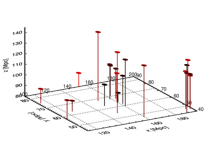
In this section we identify some of the well-known superclusters in our catalogue. The spatial distribution of REFLEX II clusters are shown in Fig. 11 in the Appendix. The clusters in the superclusters are marked in blue dots linked by lines to their BSC, and the field clusters are marked in red dots. The Shapley supercluster, known as the richest supercluster at , is found and according to the classical identification of the Shapley supercluster, it is divided into three sub-groups consisting of 21 clusters in total in our supercluster catalogue compiled with . The three-dimensional positions of the individual clusters belonging to the three sub-groups are shown in Fig. 4. The clusters are coloured according to their luminosities, the most luminous clusters are clustered in the main group in the middle. The left-most group on the x-axis is the supercluster ID 100 in Table LABEL:tab:r2cat, the large group in the middle is ID 98, and six clusters at the lower right corner belong to ID 94. We note that all three regions grow together at .
Hydra-Centaurus is located in a similar region of the sky as the Shapley supercluster, but at a lower redshift, . In our catalogue it is divided into two superclusters, ID 92 and 95 with 12 clusters in total.
Aquarius B has 16 cluster members in our sample, divided in two superclusters, ID 148 and 157. This is remarkable as it is at a redshift of , and is nearly twice as far away as Shapley. This supercluster seems to be very rich in X-ray clusters, but not extraordinarily rich in optical clusters (see EETMA).
ID 40 and 42 with 12 members altogether build the Horologium-Reticulum supercluster at and respectively. This is the largest supercluster known in the southern hemisphere. It was first reported by Shapley (1935) and studied by Lucey et al. (1983) and Chincarini et al. (1984). This supercluster is very rich in Abell clusters (see for example EETMA) and still quite rich in X-ray clusters, although less rich compared to Shapley or Aquarius B due to its larger distance.
ID 120 has seven members and a redshift . It can be identified with supercluster 172 in EETMA and supercluster 62/2 in Zucca et al. (1993). It is also one of the richest superclusters in X-rays. ID 89 at is with ten members also quite rich, which is identified with supercluster 126 in EETMA.
The superclusters at redshifts are not as rich as the nearby superclusters, as the number density of clusters decreases rapidly towards higher redshifts while the volume gets larger. The number of superclusters with more than three clusters beyond is one, between is six, and 21 for . The richest superclusters above are ID 10 at with seven clusters and ID 85 at with six clusters. There are six superclusters with five or more member clusters above =0.1.
5.2 Multiplicity function
The multiplicity function is the number of clusters found in a supercluster, which is analogous to the richness parameter for an optical cluster. We include in our catalogue already superclusters with only two members. Of course there is the question if there is more to these cluster pairs than just two clusters which are close together by chance. We attempt to answer this question in section 6 where we investigate if cluster pairs selected with a high X-ray luminosity threshold are found to be located in superclusters which have a higher multiplicity when the X-ray luminosity cut is lowered. Since the answer we find is encouraging, we take cluster pairs into our catalogue expecting that the majority of these systems would be in richer systems if the selection was extended to lower mass cluster and galaxy group regime.
The multiplicity of the REFLEX II superclusters is given in Table LABEL:tab:r2cat, and the fractional multiplicity functions are shown in Fig. 5 for a number of overdensity parameters. A large linking length corresponding to a small value of yields a larger spread in the multiplicity distribution. This is expected since a large linking length collects, by construction, clusters lying above a smaller density threshold yielding larger and richer superclusters. There are some extremely rich superclusters with more than 20 members in the top left panel of Fig. 5. For a smaller linking length corresponding to a larger overdensity, the distribution is tighter, steeply rising towards low multiplicities. This implies that this high overdensity threshold probes only the most dense areas, hence those superclusters are dominated by smaller pairs. At the largest multiplicity occurs at the core of the Shapley supercluster. It still has a multiplicity of 6 at .

The multiplicity function of our catalogue can also be understood from plot in the bottom panel of Fig. 2. With a small linking length the fraction of pair superclusters dominates the total number of superclusters while the number of richer superclusters increases clearly with a larger linking length.
Fig. 6 shows the multiplicity distribution of superclusters as a function of redshift for . The pair superclusters appear at all redshifts while richer clusters tend to segregate slightly below z=0.1. At nearly all superclusters are pair superclusters. No superclusters with more than 5 members are found at redshifts .

5.3 Extent of superclusters
The distribution of the maximum radius, Rmax, defined as half the maximum separation between the member clusters, of the REFLEX II superclusters is given in Fig. 7. The solid line denotes the distribution of the pair superclusters, and the dotted line is for the rest of richer superclusters. The distribution peaks around 10 Mpc, and the largest radius is just below 100 Mpc for the entire supercluster sample. The smallest and the largest superclusters are dominated by pair superclusters while the medium-sized supercluster distribution is equally occupied by both pair and richer superclusters. Also shown in Fig. 7 is an inset of the same distributions where the redshift is restricted to . This particular choice of the redshift cut will be explained later in Sec. 6, however, in the meantime we note that all eleven superclusters of size above 60 Mpc are located at . We have started to investigate the corresponding supercluster properties in cosmological simulations, and here we only make a short remark that the distribution of the extent of REFLEX II superclusters resembles that of the superclusters constructed from the simulation. We will defer a detailed discussion to a future publication (Chon et al., in prep.).

5.4 Comparisons with other catalogues
A direct comparison with other supercluster catalogues is not possible as this is the first time that a complete flux-limited cluster catalogue was used for the supercluster selection. Table 1 lists supercluster catalogues constructed directly with samples of galaxy clusters together with some of their properties. All catalogues except EETMA are exclusively based on Abell or Abell/ACO clusters. The early supercluster catalogues are based on relatively small cluster samples, as only a small fraction of the Abell clusters had a measured redshift. In many cases clusters with estimated redshifts were also included in the samples. Postman et al. (1992) used a sample of Abell (1958) and ACO (1989) clusters with only 15 clusters from the ACO catalogue resulting in a less complete sampling of the southern sky. Cappi & Maurogordato (1992) performed a similar analysis with a more equal coverage of the northern and southern sky, confirming the results of Postman et al. (1992) in the north.
The superclusters of all catalogues except those of Abell’s (Abell 1961) were selected using some kind of friends-of-friends analysis. Abell found superclusters by cluster counts in cells with a projected galaxy distribution for each distance class. In five catalogues the linking length depends on the overdensity and these catalogues were compiled for different overdensities, whereas for the other catalogues fixed linking lengths were used.
EETMA were the first to use X-ray selected cluster samples. Their goal was to study the clustering properties of X-ray clusters in comparison to Abell clusters. Four different X-ray cluster samples were used: the all-sky ROSAT bright survey (Voges et al., 1999), a flux-limited sample of bright clusters from the southern sky (de Grandi et al., 1999), the ROSAT brightest cluster sample from the northern sky (Ebeling et al., 1998) and a number of ROSAT pointed observations of the richest ACO clusters (David et al., 1999). The mixture of different samples produces an effective sample that is neither complete nor homogeneous. For the comparison of the clustering properties with Abell clusters this might be nevertheless a good approach. Furthermore using different samples simultaneously was at that time the only possibility to get a relatively large number of clusters, which is necessary in order to compare it with the large number of Abell clusters. EETMA give a list of 99 Abell superclusters that contain X-ray clusters of galaxies, thereof 47 superclusters in the southern hemisphere. 34 REFLEX II superclusters could be clearly identified with superclusters in that sample. Among ten additional superclusters in the non-Abell X-ray clusters by EETMA three could be identified with the REFLEX II superclusters. A number of superclusters in REFLEX II especially the very rich ones, can also be identified with superclusters in other catalogues that cover the southern sky, e.g. ZZSV or Kalinkov & Kuneva (1995).
| redshift | |||||||
| Author | #Cl | Catalogue | meas./est. | #SC | Cluster selection criteria | ||
| Abell (1961) | 1682 | Abell | 0/1682 | 17 | |||
| Rood (1976) | 27 | Abell | 27/0 | 25 | 5 | ||
| 83 | Abell | 28/0 | 25 | 15 | |||
| 166 | Abell | 8/0 | 25 | 24 | |||
| Thuan (1980) | 77 | Abell | 77/0 | 36 | , | ||
| Bahcall (1984) | 104 | Abell | 104/0 | 20 | 16 | , , | |
| Batuski & Burns (1985) | 652 | Abell | 307/345 | 40 | 102 | , | |
| West (1989) | 286 | Abell | 286/0 | 25 | 48 | , | |
| Postman et al. (1992) | 351 | Abell/ACO | 351/0 | 2 | 23 | , | |
| Cappi & Maurogordato (1992) | 233 | Abell/ACO | 219/14 | 1.9 | 24 | , , | |
| ZZSV | 4319 | Abell/ACO | 1074/3245 | 2 | 69 | h-1 Mpc, | |
| Kalinkov & Kuneva (1995) | 4073 | Abell/ACO | 1200/2873 | 10 | 893 | ||
| Einasto et al. (1994, 1997) | 1304 | Abell/ACO | 870/ 434 | 24 | 220 | , | |
| EETMA | 1663 | Abell/ACO | 1071/592 | 24 | 285 | , | |
| 497 | X-ray | 497/0 | 24 | 19 | |||
| this work | 908 | REFLEX II | 908/0 | 10 | 164 | erg s-1 cm-2 |
The fact that a significant number of superclusters are common in these catalogues constructed with significantly different selection functions shows that many of these superclusters are very characteristic and prominent structures that clearly stick out of the general cluster distribution. This is analogous to the above finding that very similar superclusters are found for a wide range of linking length.
6 Volume-limited sample
To overcome the problem of a supercluster catalogue in which the linking length varies with redshift, and in which consequently the nature of the superclusters also changes with distance, we also considered the compilation of a supercluster catalogue based on a volume-limited sample (VLS) of REFLEX II clusters. This sample has been constructed by a means of constant luminosity and redshift limit. Thus volume-limited samples of REFLEX could be any group of clusters with a luminosity and redshift limit not crossing the parabolic boundary in the – plane. Therefore the dynamical state of the superclusters from the VLS of clusters does not change with redshift. Its limitation lies in, however, small number statistics.
The VLS also gives us the chance to explore the robustness of the selection of superclusters for various selection criteria. In relation to the construction of the supercluster catalogue in the previous sections our most urgent question is the following. When going to higher redshifts, which corresponds to higher luminosity limits, the superclusters are selected from a density distribution with decreasing mean density and a larger linking length. Thus it would be important to know if we would have selected the same superclusters had we more data with a lower luminosity limit. With the VLS we can address this question by “artificially” increasing the luminosity limit (reducing the information) and by comparing the supercluster samples at increasing luminosity cuts.
The other question arises from the definition of superclusters. It is somewhat arbitrary in the sense that superclusters are not collapsed objects and their extent cannot be defined uniquely. This means that understanding the contamination in the catalogue is important. To answer this question we need a simulation to which we can apply the same selection criteria as to our REFLEX sample. In this paper, however, we take an alternative approach that utilises the REFLEX data already in hand, and defer further discussions based on simulations to the future publication (Chon et al., in prep.).
By constructing hierarchical layers of VLS with increasing lower luminosity cuts we will address the questions raised above. As a reference VLS we cut out a volume defined by and erg/s. This is one of the largest volume-limited samples that can be constructed from REFLEX IIẆith this sample we achieve a relatively high cluster density rather than the largest volume. There are in total 171 REFLEX II clusters, and we find 31 superclusters with =10. Their properties are given in Table 2. The column headings are identical to Table LABEL:tab:r2cat in the Appendix except that we identify the newly found superclusters with the superclusters in the full REFLEX II supercluster sample in Table LABEL:tab:r2cat in the eighth column.
| Supercluster | [∘] | [∘] | [Mpc] | [ erg/s] | Multiplicity | Table B.1 ID | ||
|---|---|---|---|---|---|---|---|---|
| (1) | (2) | (3) | (4) | (5) | (6) | (7) | (8) | (9) |
| RXSCJ2357-3000 | 359.459 | -30.005 | 0.0629 | 19.32 | 1.643 | 2 | 4+1 | |
| RXSCJ0013-1915 | 3.454 | -19.262 | 0.0943 | 2.66 | 1.922 | 2 | 7 | Y |
| RXSCJ0006-3414 | 1.669 | -34.235 | 0.0480 | 11.48 | 2.170 | 2 | 2 | Y |
| RXSCJ0055-1341 | 13.851 | -13.689 | 0.0550 | 28.15 | 7.992 | 4 | 13,18+1 | Y-2 |
| RXSCJ0321-4345 | 50.309 | -43.765 | 0.0707 | 34.23 | 6.096 | 4 | 39,40 | Y-2 |
| RXSCJ0357-5702 | 59.325 | -57.049 | 0.0593 | 27.98 | 8.504 | 4 | 6,42 | Y-1 |
| RXSCJ0435-3830 | 68.809 | -38.509 | 0.0516 | 19.03 | 1.249 | 2 | ||
| RXSCJ0429-1104 | 67.495 | -11.070 | 0.0356 | 16.41 | 3.015 | 2 | 50+1 | |
| RXSCJ0444-2109 | 71.083 | -21.163 | 0.0698 | 12.48 | 1.701 | 2 | 52 | |
| RXSCJ0549-2111 | 87.402 | -21.192 | 0.0958 | 21.88 | 4.739 | 4 | 61 | Y/2 |
| RXSCJ0618-5519 | 94.621 | -55.325 | 0.0539 | 24.65 | 4.013 | 4 | 62+1 | Y-1 |
| RXSCJ0913-1044 | 138.279 | -10.749 | 0.0541 | 6.57 | 6.743 | 2 | 68 | Y |
| RXSCJ1027-0945 | 156.961 | -9.759 | 0.0614 | 18.83 | 1.569 | 2 | 77+1 | |
| RXSCJ1144-1504 | 176.072 | -15.079 | 0.0722 | 12.85 | 1.230 | 2 | 84 | |
| RXSCJ1152-3259 | 178.138 | -32.987 | 0.0691 | 11.28 | 1.497 | 2 | 86 | Y |
| RXSCJ1236-3435 | 189.189 | -34.591 | 0.0770 | 13.21 | 1.326 | 2 | 90 | |
| RXSCJ1318-3055 | 199.529 | -30.923 | 0.0487 | 39.00 | 16.593 | 11 | 94,98,100 | Y/2-1 |
| RXSCJ1310-0218 | 197.746 | -2.309 | 0.0845 | 49.43 | 13.863 | 8 | 89+1 | Y/2-2 |
| RXSCJ1614-8311 | 243.631 | -83.194 | 0.0731 | 8.24 | 3.248 | 2 | 112 | Y |
| RXSCJ1704-0115 | 256.061 | -1.263 | 0.0914 | 3.98 | 2.713 | 2 | 116 | Y |
| RXSCJ2009-5513 | 302.419 | -55.231 | 0.0549 | 33.32 | 7.533 | 5 | 120+1 | Y-3 |
| RXSCJ2036-3505 | 309.066 | -35.088 | 0.0908 | 10.52 | 5.741 | 3 | 134 | Y |
| RXSCJ2226-6452 | 336.711 | -64.873 | 0.0937 | 29.83 | 5.989 | 4 | 23,156 | Y-1 |
| RXSCJ2152-5641 | 328.064 | -56.693 | 0.0780 | 30.95 | 7.511 | 6 | 145 | Y-3 |
| RXSCJ2211-0727 | 332.787 | -7.464 | 0.0854 | 46.67 | 13.247 | 10 | 148,157 | Y/2 |
| RXSCJ2147-4449 | 326.843 | -44.818 | 0.0608 | 7.33 | 1.411 | 2 | 144 | Y |
| RXSCJ2152-1937 | 328.083 | -19.625 | 0.0951 | 4.13 | 2.762 | 2 | 150 | Y |
| RXSCJ2306-1319 | 346.726 | -13.325 | 0.0670 | 4.79 | 1.150 | 2 | 160 | Y |
| RXSCJ2316-2137 | 349.030 | -21.623 | 0.0858 | 16.87 | 3.517 | 3 | 162 | Y |
| RXSCJ2318-7350 | 349.648 | -73.850 | 0.0982 | 5.29 | 1.607 | 2 | 163 | Y |
| RXSCJ2348-0702 | 357.161 | -7.048 | 0.0777 | 19.08 | 3.298 | 2 |
In addition to the reference sample we construct another three volume-limited samples with increasing lower luminosity cuts, 1, 2, and 3 erg/s. Table. 3 summarises for the different volume-limited samples our findings. As expected the number of superclusters decreases as the lower luminosity limit increases.
| Sample | LX,min [1044 erg/s] | No. REFLEX II clusters | No. Superclusters | Linking length [Mpc] |
| (1) | (2) | (3) | (4) | (5) |
| LX,0 | 0.5 | 171 | 31 | 39.3 |
| LX,1 | 1.0 | 75 | 17 | 51.7 |
| LX,2 | 2.0 | 24 | 6 | 75.6 |
| LX,3 | 3.0 | 13 | 2 | 92.7 |
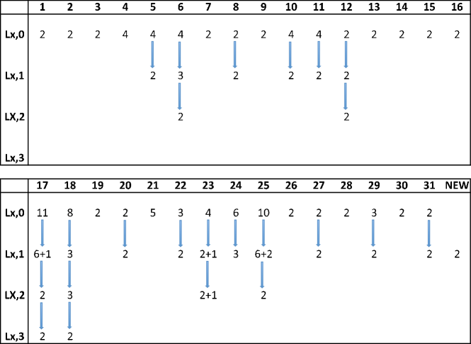
To understand how each supercluster survives a larger luminosity cut at each step we visualise this process by a tree structure shown in Fig. 8. There are two sub-tables, in which the first row records the supercluster ID as in Table 2. The rest of the rows then contain the number of member clusters in each supercluster if the supercluster was found in the specific volume-limited sample indicated by the first column. The blue arrow denotes that the supercluster from the lower luminosity cut survives up to the next higher luminosity cut. A “” denotes that the supercluster member gained an extra number of clusters that were previously not found within the same supercluster in the preceding lower luminosity cut. In summary there are 17, 6, and 2 superclusters found in the , , and samples respectively. As expected all superclusters identified at the higher luminosity cuts are found in the catalogue compiled with the lower luminosity cut with one exception, which is denoted as NEW in the last column of Fig. 8. This supercluster contains two member clusters at a maximum radius of 23 Mpc. Hence we take this as an indicator for a possible contamination in our sample.
What is interesting is then how this lower luminosity limit translates into the linking length as a function of redshift for the full sample. For each sample we have a fixed linking length, listed in column 5 of Table. 3. By combining this table and Fig. 1 we can infer that the largest lower luminosity cut of the four volume-limited samples corresponds to a redshift of 0.22. This means that the statistics that we learn from the volume-limited samples can be applied to the discussion of the full sample up to =0.22. Therefore we interpret the emergence of a new, possibly unreal supercluster in the sample of 17 superclusters as a maximum contamination of 5.8% for those 86% of the superclusters up to =0.22. We can also test how many superclusters found at redshifts are larger than 93 Mpc in diameter, and how many cluster members they contain. We find four superclusters in this range, and they are richer systems with 3 or more member clusters. Hence our sample below =0.22 does not suffer from this random spatial coincidence by not having a large pair supercluster. There is no good way to extrapolate this number out to =0.4, however, we do not expect a much larger contamination in the rest 14 % of the catalogue.
6.1 Volume fraction of superclusters
The REFLEX II supercluster catalogue includes 53% of the REFLEX II clusters, and in the VLS 62% of the clusters are associated to superclusters. We have a hint from the spatial distribution of superclusters in Fig. 11 that it is inhomogeneous. To test how much volume the superclusters take up, we calculate the volume that the superclusters occupy compared to the rest of the volume. Defining the volume of a supercluster is not unique especially for those with only pair clusters. Here we assume that superclusters occupy a spherical volume defined by the maximum radius of a supercluster as given in Tables LABEL:tab:r2cat and 2. The ratio of the volumes between the superclusters and the field is of 2% for the reference VLS, and 0.6% for the full supercluster catalogue. This is another indication that the environment occupied by the superclusters is significantly different from the field.
7 X-ray luminosity distributions
A census of the galaxy cluster population is provided by the cluster mass function. This function can be predicted on the basis of cosmic structure formation models such as the hierarchical clustering model for CDM universes by Press-Schechter type theories (Bond et al., 1991; Press & Schechter, 1974). Due to the close relation of X-ray luminosity and gravitational mass of clusters the mass function is reflected by the X-ray luminosity function (XLF) of clusters.
Thus we can use our data to study the observed XLF as a substitute for the mass function. As already mentioned in the introduction, we expect the growth of structure to continue in the dense supercluster region at a faster rate than in the field in the recent past. Thus the mass function should be more evolved. This evolution is most importantly characterised by a shift of the high mass cut-off of the mass function to higher cluster masses. We therefore expect a more top-heavy mass function and XLF for the clusters in superclusters.
The XLF of the REFLEX II clusters was derived by Böhringer et al. (2012) using the formula for the binned XLF
| (7) |
where is the size of the bin and is the survey volume, i.e. the volume defined by the survey area sr and the maximum luminosity distance , at which a cluster with a given luminosity can just be detected. Note that we have a model for which depends on the sky position to account for the varying depth of the ROSAT survey. The relationship between the survey volume and the X-ray luminosity is
| (8) |
where is the -correction.
We compare the XLF of clusters in superclusters with that of the field clusters by calculating differential and cumulative XLFs in Fig. 9. We consider two samples, the flux-limited REFLEX II sample and the VLS reference sample. Note that the two luminosity functions are normalised in a different way. For the flux-limited sample in the bottom panel of Fig. 9 all three luminosity functions (all in black, superclusters in dotted, and field in dashed line) are normalised by the total survey volume, . Thus in this plot the superclusters and field luminosity functions add up to give the total function.
For the VLS the normalisation volume is constant and does not depend on . Here we normalised the luminosity functions by the total VLS volume, by the volume occupied by superclusters as calculated in Sec. 6.1, and by the residual volume of VLS after subtraction of the supercluster volume for the total, the superclusters and the field XLF, respectively. Now the XLF of the superclusters has a normalisation about 2 orders of magnitude higher than the total function as the volume occupied by superclusters is very small while more than half of the clusters reside in superclusters. The cluster density in the field is thus lower by about a factor of 2 and so is the normalisation of the field clusters XLF.
At first glance we do not see a striking difference in the shape of the XLF. We therefore resort to a more subtle method for the comparison of the shape of the function, using a Kolmogorov-Smirnov test. We restrict this test to the VLS for the following reason. For the total REFLEX sample the XLF as shown in Fig. 9 is affected by a bias which can distort our results. A close inspection of Fig. 3 shows that the fraction of clusters in superclusters are about 60% in the lower redshift and decreases to as low as 14% at higher redshift. Since the high redshift region is only populated by very luminous clusters, the field population gets a larger share of this very luminous clusters while the superclusters get a correspondingly larger share of the less luminous nearby systems. We could in principle correct for this by normalising the luminosity function by the actual volume occupied by the superclusters. However, since the nature of the superclusters and possibly also the nature of the estimated volume changes with redshift the introduction of another bias effect can hardly be avoided.


We do not have this problem for the VLS, thus we compare the normalised cumulative XLF of clusters in superclusters, and in the field in Fig. 10. Now we see a clear effect that we have a slightly more top-heavy luminosity function in the superclusters. As the distribution functions of the cluster luminosities are un-binned, a Kolmogorov-Smirnov (KS) test was chosen to see if the luminosity distributions of field clusters and supercluster members are different. The test generally works quite well as long as the effective number of clusters . The KS probability, , lies between 0 and 1, and a small value means that the two distributions are significantly different. The KS test of the VLS yields =0.03 with a maximum separation of 0.15 at erg/s. To assess the statistical significance of this seemingly low value of in an independent way we perform a null hypothesis test with simulations. We randomly re-assign the observed luminosities of the VLS sample to clusters, and repeat the KS tests on two cumulative luminosity functions 1000 times. We find that 13% of the KS probabilities is lower than =0.03 for this null test, which corresponds roughly to 1.5 detection of a difference in the luminosity functions. We prefer to quote the latter value of the more conservative probability of the null test as the significance of our results. Hence we conclude that although the difference of the luminosity distributions of the two populations of clusters is not very large, we find an inclination for the difference using the KS test, and there are more luminous clusters in superclusters than in the field in this volume-limited sample.
We therefore find the expected over-abundance of X-ray luminous clusters in superclusters, but the effect is relatively mild. Apart from the cosmological explanation for this effect given above, we can think also of another possible explanation. In dense environments we may expect a larger frequency of cluster mergers, e.g. Richstone et al. (1992). Randall et al. (2002) analysed in hydrodynamical simulations the change of the XLF and the temperature function of merging clusters, and found that the X-ray luminosity is boosted towards higher values for about one sound crossing time during a merger event. The cumulative effect of these merger boosts affects the XLF causing an increase of the apparent number of hot luminous clusters. This boost effect has not been verified by observations, however. An important observation in this context was made by Schuecker et al. (2001), which showed that the fraction of sub-structured clusters increases with the cluster space density, analogous to the morphology segregation in clusters. Substructured clusters are the products of merging smaller clusters. Thus superclusters as regions of cluster overdensities are regions of enhanced interactions of clusters. Hence our finding that the XLF of clusters in superclusters differs from that of field clusters provides some evidence that the environment where the superclusters grow is different from the rest of our Universe. We plan to study these questions in more detail in subsequent work where we compare our observation with cosmological simulations.
8 Summary and outlook
We presented the first X-ray flux-limited supercluster catalogue based on the REFLEX II clusters. Using a friends-of-friends algorithm we explored the selection of superclusters with different overdensity parameters, and studied the properties of the supercluster catalogues. Our reference sample is constructed with , which corresponds to finding marginally bound objects given our cosmology. The resulting REFLEX II supercluster catalogue comprises 164 superclusters in the redshift range . The robustness of selection for varying linking lengths was tested by comparing to other previously known catalogues. Among the REFLEX II superclusters are the well-known nearby superclusters like Shapley and Hydra–Centaurus as well as unknown superclusters. On average these newly found superclusters have higher redshifts than what is already known with cluster of galaxies thanks to the redshift coverage of the REFLEX IIẆe compared the supercluster catalogue built with to that with , which should trace the superclusters which correspond to the bound objects that are at turn-around. All superclusters at were found in the catalogue.
We studied the multiplicity functions which show that our supercluster catalogue is largely dominated by superclusters with 5 or less cluster members from the REFLEX II cluster catalogue. Since superclusters are not collapsed objects, the definition of their volume is not unique and we decided to define the size of the superclusters by half the maximum extent of the clusters in supercluster. The distribution of this maximum radius shows that most of the superclusters are of size between 5 and 20 Mpc, and larger superclusters are dominantly found at higher redshifts.
We constructed a volume-limited sample of the REFLEX II catalogue with the constraints and 5 erg/s. This control reference sample allows us to study the effect of a volume-limited in comparison to the flux-limited supercluster catalogue. One of our findings is that increasing the luminosity cut to make a different VLS emulates the effect of redshift on the selection of superclusters in the flux-limited sample. Thus, we were able to diagnose without external data a possible contamination in the catalogue, which turns out to be a maximum statistical contamination of 5.8% in our catalogue for .
Models of structure formation imply that the supercluster environment evolves differently from the rest of the Universe. This should result in a top-heavy cluster X-ray luminosity function. Thus we studied the XLF in superclusters and the field to test this expectation. Our finding suggests that in our volume-limited sample there are more luminous clusters in superclusters, and that the volume where superclusters are found is as minuscule as less than 2% in the volume-limited sample. Hence we conclude that superclusters provide a good astrophysical ground to study the evolution of the structure growth in a distinctly dense environment. In a future publication we perform a detailed comparison to N-body simulations to better understand the properties of the X-ray superclusters and the underlying dark matter distribution.
Acknowledgments
GC acknowledges the support from Deutsches Zentrum für Luft und Raumfahrt (DLR) with the program ID 50 R 1004. We acknowledge support from the DfG Transregio Program TR33 and the Munich Excellence Cluster “Structure and Evolution of the Universe”. NN and HB acknowledge fruitful discussions with Peter Schuecker at an early stage of this work.
References
- Abell (1958) Abell, G. O. 1958, ApJS, 3, 211
- Abell (1961) Abell, G. O. 1961, AJ, 66, 607
- Abell et al. (1989) Abell, G. O., Corwin, H. G. Olowin, R. P. 1989, ApJS, 70, 1
- Balaguera-Antolínez et al. (2011) Balaguera-Antolínez, A., Sánchez, A. G., Böhringer, H., et al. 2011, MNRAS, 413, 386
- Bahcall (1984) Bahcall, N. A., Soneira, R. M. 1984, ApJ, 277, 27
- Bahcall & Burgett (1986) Bahcall, N. A., & Burgett, W. S. 1986, ApJL, 300, L35
- Bahcall (1988) Bahcall, N. A. 1988, ARA&A, 26, 631
- Bardelli et al. (2000) Bardelli, S., Zucca, E., Zamorani, G., Moscardini, L., & Scaramella, R. 2000, MNRAS, 312, 540
- Batuski & Burns (1985) Batuski, D. J., & Burns, J. O. 1985, AJ, 90, 1413
- Bogart & Wagoner (1973) Bogart, R. S., & Wagoner, R. V. 1973, ApJ, 181, 609
- Bond et al. (1991) Bond, J. R., Cole, S., Efstathiou, G., & Kaiser, N. 1991, ApJ, 379, 440
- Böhringer et al. (2000) Böhringer, H., Voges, W., Huchra, J. P., et al. 2000, ApJS, 129, 435
- Böhringer et al. (2012) Böhringer, H., Dolag, K., Chon, G., et al., 2012, A&A, 539, 120
- Böhringer et al. (2012) Böhringer, H., Chon, G., et al., 2012, in prep.
- Cappi & Maurogordato (1992) Cappi, A., & Maurogordato, S. 1992, A&A, 259, 423
- Chincarini et al. (1984) Chincarini, G., Tarenghi, M., Sol, H., et al. 1984, A&AS, 57, 1
- Chon & Böhringer (2012) Chon, G., Böhringer, H., 2012, A&A, 538, 35
- Collins et al. (2000) Collins, C., Guzzo, L., Böhringer, H. et al.: 2000, MNRAS, 319, 939
- David et al. (1999) David, L. P., Forman, W., & Jones, C. 1999, ApJ, 519, 533
- de Grandi et al. (1999) de Grandi, S., Böhringer, H., Guzzo, L., et al. 1999, ApJ, 514, 148
- Dickey & Lockman (1990) Dickey, J. M., & Lockman, F. J. 1990, ARA&A, 28, 215
- Ebeling et al. (1998) Ebeling, H., Edge, A. C., Bohringer, H., et al. 1998, MNRAS, 301, 881
- Einasto et al. (1994) Einasto, M., Einasto, J., Tago, E., Dalton, G. B., & Andernach, H. 1994, MNRAS, 269, 301
- Einasto et al. (1997) Einasto, M., Tago, E., Jaaniste, J., Einasto, J., & Andernach, H. 1997, A&AS, 123, 119
- Einasto et al. (2001) Einasto, M., Einasto, J., Tago, E., Müller, V., & Andernach, H. 2001, AJ, 122, 2222 (EETMA)
- Einasto et al. (2007) Einasto, J., Einasto, M., Tago, E., et al. 2007, A&A, 462, 811
- Hauser & Peebles (1973) Hauser, M. G., & Peebles, P. J. E. 1973, ApJ, 185, 757
- Kalinkov & Kuneva (1995) Kalinkov, M., & Kuneva, I. 1995, A&AS, 113, 451
- Liivamägi et al. (2012) Liivamägi, L. J., Tempel, E., & Saar, E. 2012, A&A, 539, A80
- Lucey et al. (1983) Lucey, J. R., Dickens, R. J., Mitchell, R. J., & Dawe, J. A. 1983, MNRAS, 203, 545
- Peebles (1974) Peebles, P. J. E. 1974, Ap&SS, 31, 403
- Postman et al. (1992) Postman, M., Huchra, J. P., & Geller, M. J. 1992, ApJ, 384, 404
- Pratt et al. (2009) Pratt, G. W., Croston, J. H., Arnaud, M., Böhringer, H. 2009, A&A, 498, 361
- Press & Schechter (1974) Press, W. H., & Schechter, P. 1974, ApJ, 187, 425
- Ragone et al. (2006) Ragone, C. J., Muriel, H., Proust, D., Reisenegger, A., & Quintana, H. 2006, A&A, 445, 819
- Randall et al. (2002) Randall, S. W., Sarazin, C. L., & Ricker, P. M. 2002, ApJ, 577, 579
- Raychaudhury et al. (1991) Raychaudhury, S., Fabian, A. C., Edge, A. C., Jones, C., & Forman, W. 1991, MNRAS, 248, 101
- Reiprich & Böhringer (2002) Reiprich, T. H., Böhringer, H. 2002, ApJ, 567, 716
- Richstone et al. (1992) Richstone, D., Loeb, A., & Turner, E. L. 1992, ApJ, 393, 477
- Rood (1976) Rood, H. J. 1976, ApJ, 207, 16
- Schechter (1976) Schechter, P. 1976, ApJ, 203, 297
- Schuecker et al. (2001) Schuecker, P., Böhringer, H., Reiprich, T. H., & Feretti, L. 2001, A&A, 378, 408
- Shapley (1935) Shapley, H. 1935, Annals of Harvard College Observatory, 88, 105
- Thuan (1980) Thuan, T. X. 1980, Physical Cosmology, 277
- Trümper (1993) Trümper, J. 1993, Science, 260, 1769
- Voges et al. (1999) Voges, W., Aschenbach, B., Boller, T., et al. 1999, A&A, 349, 389
- West (1989) West, M. J. 1989, ApJ, 347, 610
- Zucca et al. (1993) Zucca, E., Zamorani, G., Scaramella, R., & Vettolani, G. 1993, ApJ, 407, 470
Appendix A Distribution of REFLEX II superclusters
![[Uncaptioned image]](/html/1212.1597/assets/x13.png)
![[Uncaptioned image]](/html/1212.1597/assets/x14.png)
![[Uncaptioned image]](/html/1212.1597/assets/x15.png)
![[Uncaptioned image]](/html/1212.1597/assets/x16.png)


Appendix B List of REFLEX II superclusters
| Superclusters | [∘] | [∘] | [Mpc] | [1044 erg/s] | Multiplicity | =50 | ID | |
|---|---|---|---|---|---|---|---|---|
| (1) | (2) | (3) | (4) | (5) | (6) | (7) | (8) | (9) |
| RXSCJ2358-0203 | 359.546 | -2.061 | 0.0380 | 2.26 | 0.137 | 2 | Y | 1 |
| RXSCJ0006-3442 | 1.561 | -34.701 | 0.0484 | 11.48 | 2.760 | 4 | Y | 2 |
| RXSCJ0011-3557 | 2.978 | -35.957 | 0.1163 | 22.22 | 2.558 | 2 | 3 | |
| RXSCJ0013-2639 | 3.405 | -26.663 | 0.0629 | 12.95 | 1.638 | 3 | Y-1 | 4 |
| RXSCJ0022-1745 | 5.730 | -17.752 | 0.3729 | 99.50 | 21.060 | 2 | 5 | |
| RXSCJ0015-3518 | 3.933 | -35.312 | 0.0960 | 5.42 | 1.076 | 2 | Y | 6 |
| RXSCJ0013-1915 | 3.454 | -19.262 | 0.0943 | 2.66 | 1.922 | 2 | Y | 7 |
| RXSCJ0026-2031 | 6.641 | -20.529 | 0.2943 | 81.64 | 18.453 | 3 | 8 | |
| RXSCJ0024-2512 | 6.012 | -25.204 | 0.1400 | 14.91 | 4.033 | 2 | Y | 9 |
| RXSCJ0044-2727 | 11.142 | -27.461 | 0.1110 | 30.93 | 8.496 | 7 | Y-1 | 10 |
| RXSCJ0034-0014 | 8.543 | -0.244 | 0.0804 | 13.93 | 1.877 | 3 | Y-1 | 11 |
| RXSCJ0100-5004 | 15.056 | -50.071 | 0.0249 | 13.50 | 0.356 | 4 | Y-1 | 12 |
| RXSCJ0059-2143 | 14.787 | -21.723 | 0.0579 | 11.03 | 1.738 | 2 | 13 | |
| RXSCJ0107-5612 | 16.819 | -56.204 | 0.2531 | 41.39 | 8.508 | 2 | 14 | |
| RXSCJ0058-7954 | 14.534 | -79.908 | 0.1153 | 10.16 | 4.369 | 2 | Y | 15 |
| RXSCJ0105-0019 | 16.341 | -0.317 | 0.0445 | 9.91 | 2.276 | 4 | Y-1 | 16 |
| RXSCJ0104-1508 | 16.144 | -15.135 | 0.0966 | 10.07 | 1.326 | 2 | Y | 17 |
| RXSCJ0112-1441 | 18.224 | -14.687 | 0.0526 | 10.48 | 1.464 | 3 | Y | 18 |
| RXSCJ0110-4932 | 17.549 | -49.534 | 0.2052 | 26.75 | 5.310 | 2 | 19 | |
| RXSCJ0105-0016 | 16.495 | -0.276 | 0.1933 | 32.76 | 5.322 | 2 | 20 | |
| RXSCJ0111-2548 | 17.928 | -25.803 | 0.2288 | 30.02 | 10.588 | 2 | 21 | |
| RXSCJ0121-2055 | 20.495 | -20.926 | 0.1720 | 11.11 | 2.939 | 2 | Y | 22 |
| RXSCJ0125-0013 | 21.403 | -0.217 | 0.0178 | 2.45 | 0.126 | 2 | Y | 23 |
| RXSCJ0126-1758 | 21.748 | -17.970 | 0.1453 | 3.40 | 2.200 | 2 | Y | 24 |
| RXSCJ0134-1318 | 23.538 | -13.308 | 0.2069 | 13.23 | 8.393 | 2 | Y | 25 |
| RXSCJ0205-2929 | 31.441 | -29.492 | 0.3888 | 80.15 | 19.491 | 2 | Y | 26 |
| RXSCJ0153-0005 | 28.275 | -0.100 | 0.2364 | 32.55 | 8.491 | 2 | 27 | |
| RXSCJ0321-2857 | 50.390 | -28.963 | 0.0052 | 5.98 | 0.025 | 3 | Y-1 | 28 |
| RXSCJ0210-4628 | 32.503 | -46.470 | 0.0644 | 9.44 | 0.595 | 2 | 29 | |
| RXSCJ0223-4018 | 35.884 | -40.316 | 0.2234 | 32.53 | 10.907 | 2 | 30 | |
| RXSCJ0236-2755 | 39.069 | -27.929 | 0.2237 | 47.16 | 10.353 | 3 | 31 | |
| RXSCJ0234-1317 | 38.520 | -13.291 | 0.1644 | 16.00 | 2.822 | 2 | Y | 32 |
| RXSCJ0229-3320 | 37.494 | -33.343 | 0.0777 | 6.77 | 0.998 | 2 | Y | 33 |
| RXSCJ0241-0405 | 40.338 | -4.084 | 0.1866 | 29.46 | 6.699 | 2 | 34 | |
| RXSCJ0246-0030 | 41.607 | -0.503 | 0.0231 | 5.73 | 0.149 | 2 | Y | 35 |
| RXSCJ0248-2148 | 42.221 | -21.805 | 0.3175 | 42.03 | 19.670 | 2 | Y | 36 |
| RXSCJ0305-2811 | 46.341 | -28.197 | 0.2577 | 21.41 | 10.675 | 2 | Y | 37 |
| RXSCJ0309-2519 | 47.470 | -25.327 | 0.0696 | 9.72 | 0.655 | 2 | 38 | |
| RXSCJ0326-4012 | 51.640 | -40.201 | 0.0633 | 23.09 | 1.383 | 3 | 39 | |
| RXSCJ0321-4528 | 50.273 | -45.471 | 0.0731 | 21.62 | 6.624 | 7 | Y-1 | 40 |
| RXSCJ0326-5455 | 51.637 | -54.929 | 0.0835 | 14.13 | 1.987 | 2 | 41 | |
| RXSCJ0338-5414 | 54.501 | -54.245 | 0.0603 | 19.61 | 4.901 | 5 | Y-2 | 42 |
| RXSCJ0335-0157 | 53.808 | -1.957 | 0.1340 | 22.75 | 2.169 | 2 | 43 | |
| RXSCJ0342-2241 | 55.598 | -22.687 | 0.2395 | 26.40 | 8.098 | 2 | Y | 44 |
| RXSCJ0403-5408 | 60.923 | -54.150 | 0.0436 | 17.68 | 0.651 | 4 | Y/2 | 45 |
| RXSCJ0344-0249 | 56.076 | -2.826 | 0.0355 | 4.55 | 0.285 | 2 | Y | 46 |
| RXSCJ0412-0338 | 63.067 | -3.648 | 0.1381 | 13.93 | 2.897 | 2 | Y | 47 |
| RXSCJ0419-1328 | 64.792 | -13.481 | 0.2962 | 71.90 | 10.644 | 2 | 48 | |
| RXSCJ0428+0039 | 67.223 | 0.652 | 0.0138 | 6.84 | 0.219 | 3 | Y-1 | 49 |
| RXSCJ0438-1429 | 69.743 | -14.493 | 0.0334 | 8.83 | 2.317 | 3 | 50 | |
| RXSCJ0441-0035 | 70.474 | -0.593 | 0.2784 | 55.82 | 12.015 | 2 | 51 | |
| RXSCJ0445-2106 | 71.324 | -21.105 | 0.0689 | 16.47 | 1.885 | 3 | 52 | |
| RXSCJ0502-0916 | 75.719 | -9.282 | 0.2284 | 82.43 | 22.230 | 4 | 53 | |
| RXSCJ0504-0032 | 76.080 | -0.537 | 0.1245 | 18.55 | 2.870 | 2 | 54 | |
| RXSCJ0516-4610 | 79.222 | -46.176 | 0.1961 | 28.67 | 8.746 | 2 | Y | 55 |
| RXSCJ0526-3009 | 81.556 | -30.159 | 0.3310 | 64.83 | 14.020 | 2 | 56 | |
| RXSCJ0524-4124 | 81.165 | -41.416 | 0.0758 | 5.64 | 1.014 | 2 | Y | 57 |
| RXSCJ0544-2722 | 86.222 | -27.371 | 0.0408 | 21.79 | 1.463 | 5 | Y-2 | 58 |
| RXSCJ0535-3842 | 83.957 | -38.705 | 0.2906 | 95.54 | 25.664 | 3 | Y-1 | 59 |
| RXSCJ0554-3837 | 88.629 | -38.633 | 0.0463 | 11.92 | 1.540 | 3 | Y-1 | 60 |
| RXSCJ0549-2111 | 87.402 | -21.192 | 0.0958 | 21.88 | 4.739 | 4 | Y/2 | 61 |
| RXSCJ0624-5319 | 96.015 | -53.328 | 0.0520 | 26.52 | 4.243 | 8 | Y-3 | 62 |
| RXSCJ0607-5559 | 91.848 | -55.985 | 0.0362 | 10.07 | 0.157 | 2 | 63 | |
| RXSCJ0609-3454 | 92.256 | -34.914 | 0.1382 | 12.71 | 5.770 | 2 | Y | 64 |
| RXSCJ0623-4937 | 95.974 | -49.617 | 0.1194 | 23.78 | 2.806 | 3 | 65 | |
| RXSCJ0625-3717 | 96.256 | -37.293 | 0.0344 | 6.12 | 0.205 | 2 | Y | 66 |
| RXSCJ0850-0535 | 132.536 | -5.595 | 0.1842 | 36.14 | 5.557 | 3 | Y-1 | 67 |
| RXSCJ0913-1044 | 138.279 | -10.749 | 0.0541 | 6.57 | 6.743 | 2 | Y | 68 |
| RXSCJ0916-0855 | 139.161 | -8.929 | 0.2256 | 18.83 | 5.183 | 2 | Y | 69 |
| RXSCJ0933-1704 | 143.417 | -17.077 | 0.0070 | 4.10 | 0.008 | 2 | Y | 70 |
| RXSCJ1002-8242 | 150.543 | -82.701 | 0.1994 | 56.54 | 7.728 | 3 | 71 | |
| RXSCJ0929-1318 | 142.263 | -13.300 | 0.1405 | 10.58 | 2.290 | 2 | Y | 72 |
| RXSCJ0947-2536 | 146.800 | -25.614 | 0.1413 | 32.69 | 5.646 | 3 | Y-1 | 73 |
| RXSCJ0952-1049 | 148.198 | -10.822 | 0.1650 | 56.87 | 16.271 | 4 | Y-2 | 74 |
| RXSCJ1014-1405 | 153.643 | -14.096 | 0.1499 | 21.16 | 4.750 | 3 | Y | 75 |
| RXSCJ1014-0141 | 153.677 | -1.685 | 0.0433 | 11.17 | 0.493 | 2 | 76 | |
| RXSCJ1025-0934 | 156.251 | -9.572 | 0.0554 | 19.69 | 2.053 | 7 | Y/3 | 77 |
| RXSCJ1026-2652 | 156.624 | -26.877 | 0.2518 | 22.58 | 17.351 | 2 | Y | 78 |
| RXSCJ1106-2210 | 166.628 | -22.170 | 0.0640 | 4.66 | 0.711 | 2 | Y | 79 |
| RXSCJ1118-3023 | 169.577 | -30.399 | 0.1965 | 42.78 | 7.384 | 3 | 80 | |
| RXSCJ1116+0206 | 169.057 | 2.110 | 0.0749 | 8.34 | 1.349 | 2 | Y | 81 |
| RXSCJ1131-1334 | 172.808 | -13.569 | 0.1048 | 16.76 | 3.841 | 3 | Y | 82 |
| RXSCJ1135-1950 | 173.859 | -19.848 | 0.3065 | 25.97 | 24.512 | 3 | Y | 83 |
| RXSCJ1145-1620 | 176.419 | -16.345 | 0.0731 | 22.98 | 1.483 | 3 | 84 | |
| RXSCJ1200-0456 | 180.065 | -4.939 | 0.1289 | 49.62 | 6.622 | 6 | Y-4 | 85 |
| RXSCJ1152-3259 | 178.138 | -32.987 | 0.0691 | 11.28 | 1.497 | 2 | 86 | |
| RXSCJ1210+0137 | 182.595 | 1.618 | 0.0205 | 8.17 | 0.195 | 2 | 87 | |
| RXSCJ1212-2726 | 183.225 | -27.444 | 0.0822 | 8.10 | 0.769 | 2 | Y | 88 |
| RXSCJ1305-0221 | 196.451 | -2.353 | 0.0848 | 45.01 | 14.282 | 10 | Y/2-3 | 89 |
| RXSCJ1237-3429 | 189.382 | -34.490 | 0.0763 | 13.21 | 1.697 | 3 | Y-1 | 90 |
| RXSCJ1250-1529 | 192.592 | -15.493 | 0.1454 | 28.35 | 3.300 | 2 | 91 | |
| RXSCJ1316-3439 | 199.020 | -34.658 | 0.0120 | 18.57 | 1.079 | 9 | Y-2 | 92 |
| RXSCJ1255-1638 | 193.901 | -16.650 | 0.0467 | 9.12 | 2.364 | 3 | Y | 93 |
| RXSCJ1255-3012 | 193.808 | -30.204 | 0.0546 | 6.24 | 5.247 | 6 | Y | 94 |
| RXSCJ1254-1045 | 193.530 | -10.763 | 0.0151 | 2.86 | 0.087 | 3 | Y | 95 |
| RXSCJ1303-0650 | 195.918 | -6.847 | 0.1928 | 37.10 | 7.236 | 2 | 96 | |
| RXSCJ1302-2353 | 195.702 | -23.899 | 0.1284 | 6.24 | 5.036 | 2 | Y | 97 |
| RXSCJ1328-3233 | 202.216 | -32.556 | 0.0482 | 28.72 | 9.852 | 12 | Y-4 | 98 |
| RXSCJ1333-2526 | 203.462 | -25.435 | 0.1225 | 35.57 | 6.696 | 5 | Y-3 | 99 |
| RXSCJ1349-3334 | 207.327 | -33.577 | 0.0389 | 9.34 | 4.149 | 3 | 100 | |
| RXSCJ1403-1040 | 210.965 | -10.678 | 0.0707 | 17.74 | 1.407 | 3 | Y-1 | 101 |
| RXSCJ1411-1242 | 212.943 | -12.712 | 0.0995 | 12.73 | 1.889 | 2 | 102 | |
| RXSCJ1435-2821 | 218.881 | -28.356 | 0.0676 | 6.47 | 0.743 | 2 | Y | 103 |
| RXSCJ1502-0333 | 225.550 | -3.555 | 0.2164 | 29.18 | 29.656 | 2 | 104 | |
| RXSCJ1504-0954 | 226.246 | -9.901 | 0.1059 | 17.08 | 1.824 | 2 | 105 | |
| RXSCJ1505-1709 | 226.322 | -17.155 | 0.2307 | 45.18 | 20.971 | 2 | 106 | |
| RXSCJ1506-0402 | 226.712 | -4.041 | 0.0060 | 8.32 | 0.036 | 3 | Y-1 | 107 |
| RXSCJ1522-1012 | 230.660 | -10.210 | 0.0243 | 6.15 | 0.076 | 2 | 108 | |
| RXSCJ1514-2503 | 228.509 | -25.066 | 0.3256 | 68.96 | 16.131 | 2 | 109 | |
| RXSCJ1515-0044 | 228.817 | -0.739 | 0.1200 | 11.57 | 4.469 | 3 | Y | 110 |
| RXSCJ1537-0220 | 234.371 | -2.350 | 0.1516 | 18.58 | 6.861 | 3 | Y-1 | 111 |
| RXSCJ1614-8311 | 243.631 | -83.194 | 0.0731 | 8.24 | 3.248 | 2 | Y | 112 |
| RXSCJ1555-0234 | 238.806 | -2.567 | 0.1013 | 14.95 | 1.505 | 2 | 113 | |
| RXSCJ1616-0542 | 244.093 | -5.708 | 0.2050 | 23.02 | 23.607 | 2 | Y | 114 |
| RXSCJ1657-0148 | 254.478 | -1.808 | 0.0314 | 0.43 | 0.258 | 2 | Y | 115 |
| RXSCJ1704-0115 | 256.061 | -1.263 | 0.0914 | 3.98 | 2.713 | 2 | Y | 116 |
| RXSCJ1857-6605 | 284.375 | -66.090 | 0.1855 | 25.54 | 5.487 | 2 | 117 | |
| RXSCJ1913-5042 | 288.489 | -50.707 | 0.1540 | 28.64 | 4.453 | 2 | 118 | |
| RXSCJ1928-4155 | 292.010 | -41.928 | 0.0767 | 11.12 | 1.250 | 2 | 119 | |
| RXSCJ2002-5518 | 300.601 | -55.306 | 0.0554 | 21.88 | 7.699 | 7 | Y/2-1 | 120 |
| RXSCJ1940-4931 | 295.043 | -49.527 | 0.2269 | 50.97 | 10.785 | 3 | 121 | |
| RXSCJ1941-4642 | 295.285 | -46.711 | 0.2617 | 30.99 | 10.480 | 2 | Y | 122 |
| RXSCJ1950-5156 | 297.672 | -51.942 | 0.1072 | 4.51 | 2.177 | 2 | Y | 123 |
| RXSCJ1957-4405 | 299.308 | -44.090 | 0.1106 | 21.54 | 1.872 | 2 | 124 | |
| RXSCJ1956-7336 | 299.191 | -73.614 | 0.2185 | 40.34 | 12.460 | 2 | 125 | |
| RXSCJ2011-3116 | 302.819 | -31.279 | 0.1203 | 56.46 | 8.413 | 5 | Y-2 | 126 |
| RXSCJ2013-5542 | 303.330 | -55.705 | 0.2277 | 33.32 | 7.973 | 2 | 127 | |
| RXSCJ2009-3949 | 302.274 | -39.821 | 0.0191 | 2.99 | 0.097 | 2 | Y | 128 |
| RXSCJ2032-5443 | 308.052 | -54.720 | 0.1412 | 40.89 | 7.305 | 4 | 129 | |
| RXSCJ2023-3915 | 305.912 | -39.261 | 0.1455 | 41.38 | 5.079 | 3 | 130 | |
| RXSCJ2014-2500 | 303.584 | -25.007 | 0.1583 | 27.12 | 11.718 | 2 | 131 | |
| RXSCJ2015-8042 | 303.784 | -80.714 | 0.1347 | 14.28 | 3.165 | 2 | Y | 132 |
| RXSCJ2019-0655 | 304.872 | -6.920 | 0.0808 | 12.45 | 0.862 | 2 | 133 | |
| RXSCJ2037-3630 | 309.412 | -36.516 | 0.0882 | 37.66 | 7.050 | 6 | Y-3 | 134 |
| RXSCJ2101-2557 | 315.404 | -25.956 | 0.0376 | 26.24 | 0.906 | 6 | Y/2-2 | 135 |
| RXSCJ2039-2143 | 309.892 | -21.730 | 0.1999 | 22.79 | 7.306 | 2 | Y | 136 |
| RXSCJ2059-4313 | 314.944 | -43.225 | 0.0494 | 4.69 | 0.377 | 2 | Y | 137 |
| RXSCJ2103-0823 | 315.986 | -8.384 | 0.0806 | 11.46 | 0.905 | 2 | 138 | |
| RXSCJ2103-4030 | 315.992 | -40.505 | 0.1624 | 36.95 | 8.784 | 3 | Y-1 | 139 |
| RXSCJ2102-1258 | 315.640 | -12.975 | 0.0282 | 1.31 | 0.143 | 2 | Y | 140 |
| RXSCJ2104-2249 | 316.135 | -22.822 | 0.1866 | 42.45 | 13.041 | 5 | Y/2-1 | 141 |
| RXSCJ2130-2359 | 322.617 | -23.985 | 0.0652 | 19.14 | 0.765 | 3 | 142 | |
| RXSCJ2128-7340 | 322.062 | -73.674 | 0.0575 | 8.33 | 0.688 | 2 | 143 | |
| RXSCJ2143-4344 | 325.831 | -43.740 | 0.0616 | 20.04 | 1.634 | 3 | Y-1 | 144 |
| RXSCJ2150-5632 | 327.703 | -56.544 | 0.0779 | 30.95 | 8.104 | 8 | Y-4 | 145 |
| RXSCJ2135+0055 | 323.869 | 0.930 | 0.1219 | 13.96 | 2.474 | 2 | Y | 146 |
| RXSCJ2152-1815 | 328.062 | -18.250 | 0.0591 | 13.67 | 0.859 | 3 | Y-1 | 147 |
| RXSCJ2201-1020 | 330.450 | -10.348 | 0.0813 | 27.14 | 8.276 | 8 | Y-3 | 148 |
| RXSCJ2206-5559 | 331.744 | -55.985 | 0.0370 | 9.13 | 0.270 | 2 | 149 | |
| RXSCJ2152-1937 | 328.083 | -19.625 | 0.0951 | 4.13 | 2.762 | 2 | Y | 150 |
| RXSCJ2201-0603 | 330.458 | -6.052 | 0.0576 | 8.43 | 1.814 | 3 | Y | 151 |
| RXSCJ2202-2202 | 330.673 | -22.050 | 0.0708 | 8.92 | 0.978 | 2 | 152 | |
| RXSCJ2228-5200 | 337.026 | -52.002 | 0.1008 | 29.39 | 6.036 | 5 | Y/2-1 | 153 |
| RXSCJ2222-2938 | 335.652 | -29.647 | 0.0589 | 11.22 | 1.196 | 2 | 154 | |
| RXSCJ2223-3649 | 335.973 | -36.819 | 0.1494 | 33.21 | 19.595 | 4 | Y-2 | 155 |
| RXSCJ2235-6442 | 338.959 | -64.706 | 0.0941 | 12.21 | 5.736 | 4 | Y | 156 |
| RXSCJ2221-0333 | 335.436 | -3.565 | 0.0902 | 16.56 | 5.546 | 4 | Y-1 | 157 |
| RXSCJ2247-3211 | 341.830 | -32.197 | 0.2395 | 65.03 | 14.744 | 3 | 158 | |
| RXSCJ2246-1812 | 341.572 | -18.208 | 0.1299 | 34.02 | 5.573 | 3 | Y-1 | 159 |
| RXSCJ2306-1319 | 346.726 | -13.325 | 0.0670 | 4.79 | 1.150 | 2 | Y | 160 |
| RXSCJ2308-0205 | 347.093 | -2.084 | 0.2998 | 15.14 | 14.380 | 2 | Y | 161 |
| RXSCJ2316-2137 | 349.030 | -21.623 | 0.0858 | 16.87 | 3.517 | 3 | Y-1 | 162 |
| RXSCJ2318-7350 | 349.648 | -73.850 | 0.0982 | 5.29 | 1.607 | 2 | Y | 163 |
| RXSCJ2350-2650 | 357.683 | -26.844 | 0.2262 | 22.75 | 15.227 | 2 | Y | 164 |