The Glass Transition in Driven Granular Fluids: A Mode-Coupling Approach

Abstract

We consider the stationary state of a fluid comprised of inelastic hard spheres or disks under the influence of a random, momentum-conserving external force. Starting from the microscopic description of the dynamics, we derive a nonlinear equation of motion for the coherent scattering function in two and three space dimensions. A glass transition is observed for all coefficients of restitution, $\varepsilon$, at a critical packing fraction, $\varphi_{c}(\varepsilon)$, below random close packing. The divergence of timescales at the glass-transition implies a dependence on compression rate upon further increase of the density - similar to the cooling rate dependence of a thermal glass. The critical dynamics for coherent motion as well as tagged particle dynamics is analyzed and shown to be non-universal with exponents depending on space dimension and degree of dissipation.

I Introduction

A wide range of fluids can be quenched into a disordered, solid state. This includes metallic melts Greer (1995), colloidal suspensions van Megen (1995), foams Höhler and Cohen-Addad (2005) and recently, evidence was given that granular fluids may also undergo a glass transition Marty and Dauchot (2005); Abate and Durian (2006); Goldman and Swinney (2006); Reis et al. (2007); Keys et al. (2007); Kranz et al. (2010); Sperl et al. (2012). Among all these different systems, colloidal suspensions are probably best understood. Experiments by van Megen et al. Pusey and van Megen (1986); van Megen (1995) showed that besides the fluid and the ordered crystalline phase, colloidal suspensions in thermal equilibrium can also form colloidal glasses: A dynamically arrested state of the system which is characterized by diverging relaxation times Debenedetti and Stillinger (2001). While a complete theoretical understanding of the glass transition in fragile glass formers is still missing Cavagna (2009), mode coupling theories can quite successfully describe some of the phenomena on a quantitative level Götze (2009).

One interesting question has been raised more recently: Does the glass transition survive, if the system is driven by external forcing into a nonequilibrium state? Or more generally, can one observe a glass transition also in a nonequilibrium system? A well studied example are sheared colloidal suspensions for which it was shown that the equilibrium glass transition disappears Fuchs and Cates (2002, 2009). Another example is nonlinear microrheology Habdas et al. (2004); Gazuz et al. (2009); Candelier and Dauchot (2009), where a strong pulling force is applied to a single particle, forcing it out of its cage, thereby possibly melting the glass.

Another system far from equilibrium are athermal packings of particles Cates et al. (1998); Pica Ciamarra et al. (2010), undergoing a jamming transition at a critical packing fraction. Many of the properties close to the jamming point resemble those of fluids at the glass transitions. This observation is at the heart of the jamming diagram, where the glass transition in thermal systems and the jamming transition are part of a larger parameter space Liu and Nagel (1998); O’Hern et al. (2003).

Since granular particles are too large to be thermally activated, one necessarily needs a driving force to keep the grains in motion for extended periods of time. While in nature, gravity is probably the most important driving force Iverson (1997), experimentalists have devised quite a few methods of fluidisation. The list includes shaking Prevost et al. (2002), electrostatic Aranson and Olafsen (2002); Kohlstedt et al. (2005) or magnetic Kohlstedt et al. (2005); Maaß et al. (2008) excitation and fluidization by air Ojha et al. (2004); Abate and Durian (2005) or water Schröter et al. (2005).

We have recently investigated the possibility of a glass transition in driven granular fluids. In two publications Kranz et al. (2010); Sperl et al. (2012), henceforth referred to as I and II, we have demonstrated that mode coupling theory (MCT) can be generalized to the far from equilibrium stationary state of a granular fluid. In particular we found a granular glass transition for all degrees of dissipation, accompanied by the common signatures of a dense fluid close to the glass transition. Here, a careful derivation of the granular mode coupling equations is presented and the consequences of MCT are worked out in detail. We furthermore extend our previous analysis to two-dimensional systems, which are realized in many experiments on granular matter Abate and Durian (2006); Reis et al. (2007); Keys et al. (2007); Prevost et al. (2002); Abate and Durian (2005). The resulting glass transition diagram is shown in Fig. 1 in the plane spanned by packing fraction, $\varphi$, and coefficient of restitution, $\varepsilon$.

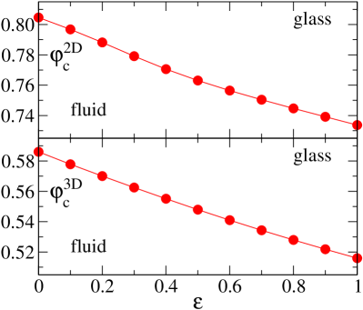
Figure 1: Critical packing fraction, $\varphi_{c}$, separating the fluid from the glassy state of driven granular particles as a function of the coefficient of restitution $\varepsilon$ for space dimension $D=2$ (top) and $D=3$ (bottom).

The dissipative interactions of the granular particles imply two primary consequences. First, while the dynamics of particles in thermal equilibrium is microscopically time reversal invariant, the symmetry under time reversal is broken for granular dynamics. Second, there is no natural equilibrium reference state like for the sheared colloids Fuchs and Cates (2002, 2009), were the fluid can be thought of as being driven out of equilibrium by the optional external driving force. In the granular system, the driving force is required to maintain a stationary state with more than transient dynamics.

The paper is organized as follows. In Sec. II we define the model of a driven granular fluid and introduce the microscopic dynamics in Sec. III. In Sec. IV we derive the MCT equations for the coherent scattering function, $\phi(q,t)$, discuss the asymptotic correlations $f_{q}:=\phi(q,t\to\infty)$, used as an order parameter to locate the glass transition, and analyze the dynamics close to the glass transition. The MCT equations for the incoherent scattering function, $\phi_{s}(q,t)$, of a tagged particle are derived in Sec. V. In Sec. VI we discuss our results in a broader context and conclude with a number of perspectives for future work in Sec. VII.

II Model

II.1 Inelastic Hard Spheres

The granular fluid is modeled as a monodisperse system of $N$ smooth inelastic hard spheres (in dimension $D=3$) or disks (in $D=2$) of radius $a$ and mass $m=1$ in a volume $V=L^{D}$. We consider the thermodynamic limit $N,V\to\infty$ such that the density $n=N/V$ remains finite. Dissipation is introduced through a constant coefficient of normal restitution $\varepsilon\in[0,1]$ that augments the law of reflection Haff (1983),

$$\hat{\bm{r}}_{12}\cdot\bm{v}^{\prime}_{12}=-\varepsilon\,\hat{\bm{r}}_{12}\cdot\bm{v}_{12},$$ (1)

where $\bm{v}_{12}=\bm{v}_{1}-\bm{v}_{2}$ is the relative velocity and $\hat{\bm{r}}_{12}$ is the unit vector pointing from the center of particle 2 to particle 1. The prime indicates post-collisional quantities.

II.2 Stochastic Driving Force

The driving force is implemented as an external random force,

$$\bm{v}^{\prime}_{i}(t)=\bm{v}_{i}(t)+\sqrt{P_{D}}\,\bm{\xi}_{i}(t),$$ (2)

where $P_{D}$ is the driving power. The $\xi_{i}^{\alpha}$, $\alpha=1,\ldots,D$ are Gaussian random variables with zero mean and variance,

$$\left\langle\xi_{i}^{\alpha}(t)\xi_{j}^{\beta}(t^{\prime})\right\rangle_{\xi}=[\delta_{ij}-\delta_{\pi(i),j}]\delta^{\alpha\beta}\delta(t-t^{\prime}),$$ (3)

where $\pi(i)=\operatorname*{arg\,min}_{k}\{|\bm{r}_{i}-\bm{r}_{k}|\geq\ell_{D}\}$ yields the index of the particle that is closest to particle $i$ but at least a given distance, $\ell_{D}$, away. Thereby, the external force does not destroy momentum conservation on length scales $\ell\gtrsim\ell_{D}$. We choose $\ell_{D}$ on the order of a mean particle separation.

II.3 The Granular Fluid

For undriven granular fluids, it is known that the homogeneous cooling state is unstable to shear- and eventually to density fluctuations McNamara (1993); Goldhirsch and Zanetti (1993). In fact, the particles form extremely dense clusters. No such clustering instability is predicted McNamara (1993), and indeed observed, for the randomly driven fluid. Consequently, we assume that the fluid is macroscopically homogeneous and isotropic. This implies that all spatial two-point correlation functions $C(\bm{r},\bm{r}^{\prime})$ are functions of the distance $|\bm{r}-\bm{r}^{\prime}|$ only. In the stationary state, the system is also time translation invariant, implying that time dependent correlation functions are only functions of time differences.

Macroscopically, the fluid is fully characterized by the packing fraction, $\varphi$ (where $\varphi=4\pi na^{3}/3$ in $D=3$ and $\varphi=\pi na^{2}$ in $D=2$), the coefficient of restitution, $\varepsilon$, and the driving power, $P_{D}$. A more conventional description is given in terms of the packing fraction and the granular temperature $T=T(\varphi,\varepsilon,P_{D})=\frac{1}{DN}\sum_{i}\bm{v}_{i}^{2}$. The latter is given by the balance between the driving power, $P_{D}$, and the energy loss through the inelastic collisions, $P_{\varepsilon}:=\Pi_{\varepsilon}(\varphi,\varepsilon)\omega_{c}T$, where $\Pi_{\varepsilon}(\varphi,\varepsilon)\simeq\Pi_{\varepsilon,E}(\varepsilon)=(1-\varepsilon^{2})/D$ in a mean field approximation Haff (1983).

The collision frequency $\omega_{c}\propto\sqrt{T}$ is the only time scale of the system. Thus, changing the granular temperature only changes the time scale of the system. To keep the discussion more transparent, we refrain from using the freedom to set $T=1$ but keep in mind that the qualitative behavior of the system is independent of the temperature $T>0$.

III Microscopic Description

III.1 Observables

The two relevant observables discussed in the following are the density field, $\rho(\bm{r},t)$, and the current density, $\bm{j}(\bm{r},t)$, with the following microscopic definitions:

$$\rho(\bm{r},t) =\frac{1}{N}\sum_{i}\delta(\bm{r}-\bm{r}_{i}(t)),$$ (4a)

$$\bm{j}(\bm{r},t) =\frac{1}{N}\sum_{i}\bm{v}_{i}(t)\delta(\bm{r}-\bm{r}_{i}(t)).$$ (4b)

We will use the spatial Fourier transforms $\rho_{\bm{k}}(t)=\textsf{FT}[\rho](t)$ and the longitudinal current $j_{\bm{k}}^{L}(t)=\hat{\bm{k}}\cdot\textsf{FT}[\bm{j}](t)$. The corresponding tagged particle quantities are given as

$$\rho^{s}(\bm{r},t) =\delta(\bm{r}-\bm{r}_{s}(t)),$$ (5a)

$$\bm{j}^{s}(\bm{r},t) =\bm{v}_{s}\delta(\bm{r}-\bm{r}_{s}(t)).$$ (5b)

III.2 Dynamics

The (forward in time) pseudo Liouville operator $\mathcal{L}_{+}$ describes the time evolution of a microscopic observable $A$, i.e., $i\mathcal{L}_{+}A=dA/dt$, according to the dynamics specified above Altenberger (1975). It is given as the sum of three parts,

$$\mathcal{L}_{+}=\mathcal{L}_{0}+\sum_{j<k}\mathcal{T}_{jk}^{+}+\mathcal{L}_{D}^{+},$$ (6)

which are in turn: (i) The free streaming operator $i\mathcal{L}_{0}=\sum_{j}\bm{v}_{j}\cdot\nabla_{j}$. (ii) The collision operator,

$$i\mathcal{T}_{jk}^{+}=-(\hat{\bm{r}}_{jk}\cdot\bm{v}_{jk})\Theta(-\hat{\bm{r}}_{jk}\cdot\bm{v}_{jk})\delta(r_{jk}-2a)(b_{jk}^{+}-1),$$ (7)

where $\Theta(x)$ denotes the Heaviside step function and the operator $b_{jk}^{+}$ implements the inelastic collision rule Aspelmeier et al. (2001) and (iii) the driving operator ,

$$i\mathcal{L}_{D}^{+}= \sqrt{P_{D}}\sum_{j}\bm{\xi}_{j}(t)\cdot\left(\frac{\partial}{\partial\bm{v}_{j}}-\frac{\partial}{\partial\bm{v}_{\pi(j)}}\right)$$ (8)

$$+P_{D}\sum_{j}\frac{\partial^{2}}{\partial\bm{v}_{j}^{2}}.$$

With the binary collision expansion Ernst et al. (1969), formal power series of the pseudo Liouville operator can be defined. In particular, this allows to write the propagator $\mathsf{U}(t)=\exp(it\mathcal{L}_{+})$ in terms of an exponential operator $\exp(it\mathcal{L}_{+}):=\sum_{n}(it\mathcal{L}_{+})^{n}/n!$. The Laplace transformed propagator $\hat{\mathsf{U}}(s)\equiv\textsf{LT}[\mathsf{U}](s)=(s-\mathcal{L}_{+})^{-1}$ is then also defined as a power series .

The starting point for the derivation of equations of motion is an operator identity that is most concisely expressed in the Laplace domain,

$$\mathcal{P}\hat{\mathsf{U}}(s)\mathcal{P}=[s-\mathsf{\Omega}-\hat{\mathsf{M}}(s)]^{-1},$$ (9)

where $\mathsf{\Omega}=\mathcal{P}\mathcal{L}_{+}\mathcal{P}$,

$$\mathsf{M}(t)=\mathcal{P}\mathcal{L}_{+}\mathcal{Q}\exp(it\mathcal{Q}\mathcal{L}_{+}\mathcal{Q})\mathcal{Q}\mathcal{L}_{+}\mathcal{P},$$ (10)

and $\mathcal{P}=\mathcal{P}^{2},\mathcal{Q}=1-\mathcal{P}$ are projection operators Mori (1965).

III.3 Phase Space Averages

Our approach starts from the microscopic description of the particle dynamics in terms of the location in phase space, $\Gamma:=(\bm{r}_{1},\bm{v}_{1},\ldots\bm{r}_{N},\bm{v}_{N})$ and the trajectory of the external driving force $\Xi_{t}=(\bm{\xi}_{1}(t),\ldots,\bm{\xi}_{N}(t))$. Macroscopic observables $\tilde{A}(\bm{r},t|\Xi_{t}):=\left\langle a(\bm{r},t|\Gamma,\Xi_{t})\right\rangle_{\Gamma}\equiv\int d\Gamma\varrho(\Gamma,t)a(\bm{r},t|\Gamma,\Xi_{t})$ are then introduced as expectation values with respect to the phase space distribution function $\varrho(\Gamma,t)$ of the microscopic variables. Here, we restrict ourselves to the stationary state, where the distribution function is time independent, $\varrho(\Gamma,t)\equiv\varrho(\Gamma)$.

In contrast to fluids in equilibrium, no analytical expression for the stationary phase space distribution of driven granular fluids is known so far. Therefore we have to make a few assumptions to evaluate the expectation values. First of all we assume that positions and velocities are uncorrelated, $\varrho(\Gamma)=\varrho_{r}(\{\bm{r}_{i}\})\varrho_{v}(\{\bm{v}_{i}\})$. Moreover, we assume that the velocity distribution factorizes into a product of one particle distribution functions, $\varrho_{v}(\{\bm{v}_{i}\})=\prod_{i}\varrho_{1}(\bm{v}_{i})$. All we need to know about $\varrho_{1}(\bm{v})$ is that it has a vanishing first moment, $\int d^{D}v\,\bm{v}\varrho_{1}(\bm{v})=0$ and a finite second moment, $\int d^{D}v\,v^{2}\varrho_{1}(\bm{v})=DT<\infty$. The spatial distribution function, $\varrho_{r}(\{\bm{r}_{i}\})$, enters the theory via static correlation function, as will be discusssed below.

A common expectation in disordered systems is, that the macroscopic expectation values should be self averaging, i.e., independent of any specific disorder realization Brout (1959). In our model, this applies to the stochastic driving force $\Xi_{t}$, i.e., we define macroscopic observables as averages over all realizations of the driving, $A(\bm{r},t)=\left\langle a(\bm{r},t)\right\rangle:=\left\langle\tilde{A}(\bm{r},t|\Xi_{t})\right\rangle_{\xi}\equiv\int d\Xi_{t}P(\Xi_{t})\tilde{A}(\bm{r},t|\Xi_{t})$. Here, $P(\Xi_{t})$ is the distribution of the random forces. Averages over pairs of observables define a scalar product, $\left\langle A|B\right\rangle:=\left\langle A^{*}B\right\rangle$ where $A^{*}$ denotes the complex conjugate of $A$.

Given the definition of a scaler product, we can formally introduce the adjoint Liouville operator, $\mathcal{L}_{+}^{\dagger}$, via the relation $\left\langle\mathcal{L}_{+}^{\dagger}a|b\right\rangle=\left\langle a|\mathcal{L}_{+}b\right\rangle$. For elastic hard spheres in thermal equilibrium, it can be shown that detailed balance implies $\mathcal{L}_{+}^{\dagger}(\varepsilon=1)=\mathcal{L}_{-}(\varepsilon=1)$, where $\mathcal{L}_{-}$ is the Liouville operator describing time reversed dynamics. This relation does not hold for inelastic collisions which are discussed here. In the present context, an explicit expression for $\mathcal{L}_{+}^{\dagger}$ is not needed and hence will be given elsewhere.

As both the hard sphere interactions and the driving force (by construction) conserve momentum, this will also be reflected in the matrix elements $\left\langle a_{1}(\bm{k}_{1})\cdots a_{n}(\bm{k}_{n})|b_{1}(\bm{p}_{1})\cdots b_{m}(\bm{p}_{m})\right\rangle\propto\delta_{\sum\bm{k}_{i},\sum\bm{p}_{i}}$ in the form of a selection rule.

The central quantities in the following will be the coherent scattering function

$$\phi(q,t):=N\left\langle\rho_{\bm{q}}(\tau)|\rho_{\bm{q}}(\tau+t)\right\rangle/S_{q},$$ (11a)

where $$S_{q}:=N\left\langle\rho_{\bm{q}}|\rho_{\bm{q}}\right\rangle$$ is the static structure factor, and the incoherent scattering function

$$\phi_{s}(q,t):=\left\langle\rho_{\bm{q}}^{s}(\tau)|\rho_{\bm{q}}^{s}(\tau+t)\right\rangle.$$ (11b)

In general, all macroscopic quantities will be functions of the coefficient of restitution $\varepsilon$. To reduce clutter, we will suppress this dependence.

III.4 Static Structure Factors

Below, we will treat the static structure functions as a known input. Hence, we need $S_{q}=S_{q}(\varphi,\varepsilon)$ for a range of densities, $\varphi$ around where we expect the critical density to be. Lacking good quality data for $S_{q}(\varphi\sim\varphi_{c}(\varepsilon),\varepsilon)$, let alone reliable theoretical predictions for this quantity, we use preliminary results that $S_{q}(\varphi,\varepsilon)$ only weakly depends on the coefficient of restitution $\varepsilon$ and approximate $S_{q}(\varphi,\varepsilon)\approx S_{q}(\varphi,\varepsilon=1)$ by their elastic counterparts: In $D=3$ we use the Percus-Yevick (PY) equation Percus and Yevick (1958) for elastic hard spheres in thermal equilibrium Ashcroft and Lekner (1966), except for the pair correlation function at contact which is better approximated by the Carnahan-Starling expression Carnahan and Starling (1969). In $D=2$ we use the Baus-Colot (BC) equation Baus and Colot (1987) throughout.

IV The Granular Glass Transition

IV.1 Equations of Motion

Let us introduce the following microscopic state vector $\bm{a}_{\bm{q}}=\sqrt{N}(\rho_{\bm{q}}/\sqrt{S_{q}},j_{\bm{q}}^{L}/\sqrt{T})$. Then the coherent scattering function $\phi(q,t)$ is given as one element of the matrix of correlators $\Phi(q,t)=\left\langle\bm{a}_{\bm{q}}|\mathsf{U}(t)\bm{a}_{\bm{q}}\right\rangle$.

With the help of Eq. (9) and the projectors

$$\mathcal{P}_{c}=N\sum_{\bm{q}}\left|\rho_{\bm{q}}\right\rangle\left\langle\rho_{\bm{q}}\right|/S_{q}+N\sum_{\bm{q}}\left|j_{\bm{q}}^{L}\right\rangle\left\langle j_{\bm{q}}^{L}\right|/T,$$ (12)

$\mathcal{Q}_{c}=1-\mathcal{P}_{c}$, one finds

$$\hat{\Phi}^{-1}(q,s)=\begin{pmatrix}s&-\Omega_{\rho j}(q)[1+\hat{L}(q,s)]\\ -\Omega_{j\rho}(q)&s-\nu_{q}-\hat{M}(q,s)\end{pmatrix},$$ (13)

while $\Omega_{\rho\rho}\propto\left\langle\rho_{\bm{q}}|\mathcal{L}_{+}\rho_{\bm{q}}\right\rangle=q\left\langle\rho_{\bm{q}}|j_{\bm{q}}^{L}\right\rangle=0$ due to parity. The other entries of the frequency matrix $\Omega_{ab}=\left\langle\bm{a}_{\bm{q}}|\mathsf{\Omega}\bm{a}_{\bm{q}}\right\rangle$ are nonzero [Note that $\nu_{q}=\Omega_{jj}(q)$].

The memory kernels are formally given as

$$M(q,t) =N\left\langle F_{\bm{q}}^{\dagger}\tilde{\mathsf{U}}(t)F_{\bm{q}}\right\rangle/T,$$ (14a)

$$L(q,t) =\left\langle J_{\bm{q}}^{\dagger}\tilde{\mathsf{U}}(t)F_{\bm{q}}\right\rangle/q\left\langle j_{\bm{q}}^{L}|j_{\bm{q}}^{L}\right\rangle,$$ (14b)

where $\tilde{\mathsf{U}}(t)=\exp(it\mathcal{Q}_{c}\mathcal{L}_{+}\mathcal{Q}_{c})$ is a modified propagator. There are two fluctuating forces, $F_{\bm{q}}=\mathcal{Q}_{c}\mathcal{L}_{+}j_{\bm{q}}^{L}$, and $F_{\bm{q}}^{\dagger}=\mathcal{Q}_{c}\mathcal{L}_{+}^{\dagger}j_{\bm{q}}^{L}$, and at this point we can not rule out that there is a nonzero fluctuating current, $J_{\bm{q}}^{\dagger}=\mathcal{Q}_{c}\mathcal{L}_{+}^{\dagger}\rho_{\bm{q}}$, while $J_{\bm{q}}=\mathcal{Q}_{c}\mathcal{L}_{+}\rho_{\bm{q}}=q\mathcal{Q}_{c}j_{\bm{q}}^{L}=0$. In the elastic limit $F_{\bm{q}}^{\dagger}=F_{\bm{q}}$ and $J_{\bm{q}}^{\dagger}=J_{\bm{q}}=0$ holds and therefore $L(q,t)$ vanishes.

In the Laplace domain, the coherent scattering function is thus given as

$$\hat{\phi}^{-1}(q,s)=s-\frac{\Omega_{q}^{2}[1+\hat{L}(q,s)]}{s-\nu_{q}-\hat{M}(q,s)},$$ (15)

where $\Omega_{q}^{2}=\Omega_{\rho j}\Omega_{j\rho}$, or, equivalently, in the time domain as the solution of the equation of motion,

$$\ddot{\phi}(q,t) +\nu_{q}\dot{\phi}(q,t)+\Omega_{q}^{2}\phi(q,t)$$ (16)

$$+\Omega_{q}^{2}\int_{0}^{t}\!d\tau\,m(q,t-\tau)\dot{\phi}(q,\tau)$$

$$+\Omega_{q}^{2}\int_{0}^{t}\!d\tau\,L(q,t-\tau)\phi(q,\tau)=0,$$

where $m(q,t)=M(q,t)/\Omega_{q}^{2}$ and the initial conditions are $\dot{\phi}(q,t=0)=0$ and $\phi(q,t=0)=1$. To proceed, we need to find approximate expressions for the memory kernels. Before we come to the mode coupling approximation, we discuss the simpler assumption that $M(q,t)=L(q,t)=0$.

IV.2 Sound Waves

The linear equation of motion

$$\ddot{\phi}(q,t)+\nu_{q}\dot{\phi}(q,t)+\Omega_{q}^{2}\phi(q,t)=0$$ (17)

describes damped sound waves $\phi(q,t)=e^{-\nu_{q}t/2}\cos(C_{q}qt)$.

Sound damping due to collisions, as described by the second term in Eq. (17),

$$\nu_{q}=N\left\langle j_{\bm{q}}^{L}|\mathcal{L}_{+}j_{\bm{q}}^{L}\right\rangle/T,$$ (18)

can be evaluated in the Enskog approximation. The calculation for two dimensions is shown in appendix B.1, yielding

$$\nu_{q}=\frac{1+\varepsilon}{2}\omega_{E}[1+2J_{0}^{\prime\prime}(2aq)]\quad\quad\text{in $D=2$,}$$ (19a)

where $$J_{0}(x)$$ is the zeroth order Bessel function Jeffrey and Zwillinger (2000) and the double prime denotes the second derivative with respect to the argument. The result in three dimensions is known Leutheusser (1982),

$$\nu_{q}=\frac{1+\varepsilon}{3}\omega_{E}[1+3j_{0}^{\prime\prime}(2aq)]\quad\quad\text{in $D=3$,}$$ (19b)

where $j_{0}(x)=\sin(x)/x$ is the zeroth order spherical Bessel function . The Enskog collision frequency $\omega_{E}=2^{D}D(\varphi\chi/2a)\sqrt{T/\pi}$ is given in terms of the contact value, $\chi$, of the pair correlation function Hansen and McDonald (2006).

The speed of sound is given in the long wavelength limit by $C_{q}^{2}=\Omega_{q}^{2}/q^{2}=\Omega_{\rho j}\Omega_{j\rho}/q^{2}$. One finds,

$$\Omega_{j\rho} =N\left\langle j_{\bm{q}}^{L}|\mathcal{L}_{+}\rho_{\bm{q}}\right\rangle/\sqrt{TS_{q}}$$ (20a)

$$=qS_{\ell\ell}(q)\sqrt{T/S_{q}}$$

with the longitudinal current correlator $$S_{\ell\ell}(q):=N\left\langle j_{\bm{q}}^{L}|j_{\bm{q}}^{L}\right\rangle/T$$. The calculation (cf. appendix B.2) of

$$\Omega_{\rho j} =\frac{N}{\sqrt{TS_{q}}}\left\langle\rho_{\bm{q}}|\mathcal{L}_{+}j_{\bm{q}}^{L}\right\rangle$$ (20b)

$$\approx q\sqrt{T/S_{q}}\left(\frac{1+\varepsilon}{2}+\frac{1-\varepsilon}{2}S_{q}\right)$$

uses the approximate granular Yvon-Born-Green (YBG) relation (cf. appendix A). Combining these results, we find that the long wavelength speed of sound,

$$C_{q}^{2}=T\frac{S_{\ell\ell}(q)}{S_{q}}\left(\frac{1+\varepsilon}{2}+\frac{1-\varepsilon}{2}S_{q}\right),$$ (21)

is reduced for the dissipative driven fluid compared to a fluid of elastic hard spheres in thermal equilibrium. The sound damping, $\nu_{q}/2q^{2}$, on the other hand decreases with increasing dissipation.

Alternatively, the speed of sound can be given as $C_{q}^{2}=S_{\ell\ell}(q)/n\kappa_{q}^{\mathrm{eff}}$, where the effective compressibility $\kappa_{q}^{\mathrm{eff}}$ is defined in a form,

$$\frac{1}{\kappa_{q}^{\mathrm{eff}}}=\frac{1}{\kappa_{q}^{0}}+\frac{1-\varepsilon}{2}Tn^{2}c_{q},$$ (22)

reminiscent of a random phase approximation Schweizer and Curro (1988). Here, $\kappa_{q}^{0}=S_{q}/nT$ is the compressibility of a fictitious elastic hard sphere system with a structure factor $S_{q}$ and $c_{q}$ is the direct correlation function Hansen and McDonald (2006).

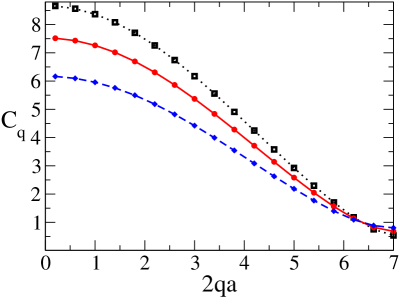
Figure 2: Speed of sound, $C_{q}$, according to Eq. (21) as a function of wave number, $q$, in 3D for packing fraction $\varphi=0.516$ and coefficient of restitution $\varepsilon=1.0$ (squares), 0.5 (filled circles), and 0.0 (diamonds).

We close this section with a few remarks. First, in a thermal fluid the expression for the sound velocity simplifies, because $S_{\ell\ell}(q)\equiv 1$ due to molecular chaos Boon and Yip (1992). In a granular fluid, $S_{\ell\ell}(q)$ is actually found to be wave number dependent. Preliminary results indicate $S_{\ell\ell}(q\to 0)<1$. Second, from $\Omega_{\rho j}\neq\Omega_{j\rho}$ for $\varepsilon<1$, it can be seen explicitly that the Liouville operator is not self adjoint. In terms of physical processes, this reflects that the transition rate for the conversion of density fluctuations into current fluctuations is not equal to the rate of the reverse process. Detailed balance, or more general, time reversal invariance it broken already for the linear equation of motion (cf. Sec. V.1 below). Finally, it is known Hansen and McDonald (2006) that Navier-Stokes-order hydrodynamics does not exist in $D=2$, presumably implying logarithmic corrections to the sound damping in $D=2$.

In the following, we set $S_{\ell\ell}(q)\equiv 1$. In Fig. 2, the resulting sound dispersion relations are shown for packing fraction $\varphi=0.516$ and coefficient of restitution varying from $\varepsilon=1$ to 0. The speed of sound decreases with increasing dissipation in agreement with hydrodynamic predictions van Noije et al. (1999).

IV.3 The Mode Coupling Approximation

In the spirit of the equilibrium mode coupling theories Fixman (1962); Kawasaki (1966); Kadanoff and Swift (1968); Bosse et al. (1978), we introduce a second projection operator

$$\mathcal{P}_{2}=N^{2}\sum_{\bm{k},\bm{p}}\left|\rho_{\bm{k}}\rho_{\bm{p}}\right\rangle\left\langle\rho_{\bm{k}}\rho_{\bm{p}}\right|/S_{k}S_{p}$$ (23)

and approximate the modified propagator as

$$\tilde{\mathsf{U}}(t) \approx\mathcal{P}_{2}\tilde{\mathsf{U}}(t)\mathcal{P}_{2}$$ (24)

$$\approx N^{2}\sum_{\bm{k},\bm{p}}\left|\rho_{\bm{k}}\rho_{\bm{p}}\right\rangle\phi(k,t)\phi(p,t)\left\langle\rho_{\bm{k}}\rho_{\bm{p}}\right|/S_{k}S_{p},$$

where in the second step, a factorization approximation, $N^{2}\left\langle\rho_{\bm{k}}\rho_{\bm{p}}|\tilde{\mathsf{U}}(t)\rho_{\bm{k}}\rho_{\bm{p}}\right\rangle/S_{k}S_{p}\approx\phi(k,t)\phi(p,t)$, was employed. Eq. (24) is known as the mode coupling approximation (MCA).

IV.3.1 The MCA of $L$

We find

$$L(q,t)\approx\frac{N}{qT}\sum_{\bm{k},\bm{p}}\mathcal{U}_{\bm{q}\bm{k}\bm{p}}\mathcal{W}_{\bm{q}\bm{k}\bm{p}}\phi(k,t)\phi(p,t),$$ (25)

where

$$\mathcal{U}_{\bm{q}\bm{k}\bm{p}}=N\left\langle\rho_{q}|\mathcal{L}_{+}\mathcal{Q}_{c}\rho_{k}\rho_{p}\right\rangle/S_{k}=0$$ (26)

due to parity and $\mathcal{W}_{\bm{q}\bm{k}\bm{p}}$ is defined below. Therefore $L(q,t)\equiv 0$ within the mode coupling approximation.

IV.3.2 The MCA of $M$

The mode coupling approximation for $M(q,t)$ yields

$$M(q,t)\approx\frac{N}{T}\sum_{\bm{k},\bm{p}}\mathcal{V}_{\bm{q}\bm{k}\bm{p}}\mathcal{W}_{\bm{q}\bm{k}\bm{p}}\phi(k,t)\phi(p,t),$$ (27)

where

$$\mathcal{V}_{\bm{q}\bm{k}\bm{p}} =N\left\langle j_{\bm{q}}^{L}|\mathcal{L}_{+}\mathcal{Q}_{c}\rho_{\bm{k}}\rho_{\bm{p}}\right\rangle/S_{k},$$ (28a)

$$\mathcal{W}_{\bm{q}\bm{k}\bm{p}} =N\left\langle\rho_{\bm{k}}\rho_{\bm{p}}|\mathcal{Q}_{c}\mathcal{L}_{+}j_{q}^{L}\right\rangle/S_{p}.$$ (28b)

The left vertex is known from the literature Barrat et al. (1989)

$$\mathcal{V}_{\bm{q}\bm{k}\bm{p}}=\frac{T}{NS_{k}}[(\hat{\bm{q}}\cdot\bm{k})S_{p}+(\hat{\bm{q}}\cdot\bm{p})S_{k}-qS^{(3)}(\bm{k},\bm{p})/S_{q}]\delta_{\bm{q},\bm{k}+\bm{p}}.$$

Customarily, the convolution approximation Jackson and Feenberg (1962), $S^{(3)}(\bm{k},\bm{p})\approx S_{k}S_{p}S_{q}$, is applied to yield

$$\mathcal{V}_{\bm{q}\bm{k}\bm{p}}=\frac{T}{N}S_{p}[(\hat{\bm{q}}\cdot\bm{k})nc_{k}+(\hat{\bm{q}}\cdot\bm{p})nc_{p}]\delta_{\bm{q},\bm{k}+\bm{p}}.$$ (29a)

By a nontrivial calculation (see appendix B.3), we were able to show that the right vertex is approximately given as

$$\mathcal{W}_{\bm{q}\bm{k}\bm{p}}\approx\frac{1+\varepsilon}{2}\frac{T}{N}S_{k}[(\hat{\bm{q}}\cdot\bm{k})nc_{k}+(\hat{\bm{q}}\cdot\bm{p})nc_{p}]\delta_{\bm{q},\bm{k}+\bm{p}},$$ (29b)

different from$\mathcal{V}_{\bm{q}\bm{k}\bm{p}}$.

The physical interpretation of these results for the vertices is, that (i) the rate of annihilation of pairs of density fluctuations $\rho_{\bm{k}},\rho_{\bm{p}}$ is determined by the static structure of the fluid, both in an equilibrium fluid and in the driven granular fluid; (ii) The rate of creation of such density fluctuations is suppressed by a factor $(1+\varepsilon)/2$, though, compared to the rate of creation or to the equivalent rate in an equilibrium fluid.

The reduced memory kernel in the mode coupling approximation (first reported in I) then reads

$$m[\phi](q,t)=A_{q}(\varepsilon)\frac{nS_{q}}{q^{2}}\int d^{D}k\,S_{k}S_{|\bm{q}-\bm{k}|}\left\{[\hat{\bm{q}}\cdot\bm{k}]c_{k}+[\hat{\bm{q}}\cdot(\bm{q}-\bm{k})]c_{p}\right\}^{2}\phi(k,t)\phi(|\bm{q}-\bm{k}|,t),$$ (30)

where

$$A^{-1}_{q}(\varepsilon)=1+\frac{1-\varepsilon}{1+\varepsilon}S_{q}.$$ (31)

Fig. 3 demonstrates the prefactor $A_{q}(\varepsilon)$ that distinguishes the granular memory functions from the well-known elastic results where $A_{q}(\varepsilon=1.0)=1$: For $\varepsilon<1$, the prefactor exhibits deviations from unity with oscillations given by the static structure factor. As $A_{q}(\varepsilon)$ is minimal for the first peak of the structure factor, i.e. the length scale of the cage, one concludes that increasing dissipation (decreasing coefficient of restitution) weakens the cage effect. Compared to the elastic case, the force acting by the cage onto the particles inside the cage is smaller as the particles’ reflections from each other are reduced by the influence of dissipation. While additional changes are expected by the $\varepsilon$-dependence of the structure factors, the major difference is encoded in the prefactor $A_{q}(\varepsilon)$. The fact that $A_{q}(\varepsilon)>0$ for all values of the coefficient of restitution $\varepsilon$ ensures that the memory kernel remains positive.

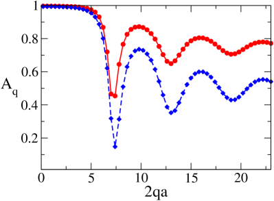
Figure 3: Prefactor of the memory kernel, $A_{q}(\varepsilon)$, as a function of wave number, $q$, for two values of the coefficient of restitution, $\varepsilon=0.5$ (filled circles) and 0.0 (diamonds), in 3D.

IV.4 The approximate equation of motion and the phase diagram

With the mode coupling approximations in place, the equation of motion

$$\ddot{\phi}(q,t) +\nu_{q}\dot{\phi}(q,t)+\Omega_{q}^{2}\phi(q,t)$$ (32)

$$+\Omega_{q}^{2}\int_{0}^{t}\!d\tau\,m[\phi](q,t-\tau)\dot{\phi}(q,\tau)=0$$

turns into a closed equation for the coherent scattering function once the static structure factor, $S_{q}$, is known. This equation of motion has the same formal structure as the one for the elastic hard sphere fluid in thermal equilibrium. The viscous term, Eq. (18), decreases with decreasing coefficient of restitution $\varepsilon$; the speed of sound, Eq. (21), acquires a nontrivial dependence on the coefficient of restitution as does the memory kernel $m[\phi]$.

Structural arrest of the grains in a glassy state gives rise to time persistent density correlations. Hence, we introduce the order parameter for the glass transition, $f_{q}:=\lim_{t\to\infty}\phi(q,t)$. It can readily be shown that the above equation of motion yields the following equation for the asymptotic function, $f_{q}$,

$$\frac{f_{q}}{1-f_{q}}=m[f](q).$$ (33)

With the memory kernel being independent of temperature, the order parameter $f_{q}$ is also independent of temperature as expected. It can easily be checked, that $f_{q}\equiv 0$ is always a solution of the above equation. Studying this equation from a dynamical systems point of view, one finds that at a critical density $\varphi_{c}$, the vanishing solution becomes unstable and a new, stable solution $f_{q}>0$ appears discontinuously, signaling the glass transition Götze (2009). The order parameter at the critical density $\varphi_{c}$ will be denoted as $f_{q}^{c}$.

Using the structure factors as discussed in Sec. III.4, we find the phase diagrams in Fig. 1. For $D=3$ this result was first reported in I, whereas for $D=2$ this is a new result (for technical parameters, cf. appendix C). The order parameter jumps discontinuously at the critical density $\varphi_{c}$ as expected Götze (2009) from the type of singularity in Eq. (33). The evolution of the transition with $\varepsilon$ is remarkably similar for 2D and 3D, with transition densities increasing from the elastic case to $\varepsilon=0.0$ by around 10% in a roughly linear fashion.

IV.5 Coherent Dynamics Close to the Glass Transition

The full dynamics of density fluctuations is obtained by solving the MCT equations by iteration (for details, see Appendix C). In Figs. 4 and 5 we show the coherent scattering function in $D=3$ for several densities, below and above the critical point for $\varepsilon=0.5$ and two wave numbers $2qa=4.2$ and $2qa=7$. As the critical point is approached from the fluid side, one observes the development of a plateau in the coherent scattering function. Increasing the density above the critical value $\varphi_{c}$ leads to an increase in the order parameter, $f_{q}$ Franosch et al. (1997).

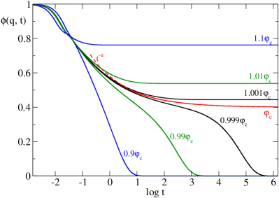
Figure 4: Coherent scattering functions, $\phi(q,t)$, as a function of time, $t$, in 3D for wave number $q=4.2/2a$. At the transition point at packing fraction $\varphi^{c}(\varepsilon=0.5)=0.548$ with a critical glass-form factor of $f_{q}^{c}=0.400$, and at higher ($1.1\varphi^{c}$, $1.01\varphi^{c}$, $1.001\varphi^{c}$) and lower ($0.9\varphi^{c}$, $0.99\varphi^{c}$, $0.999\varphi^{c}$) packing fractions. The exponent parameter is $\lambda=0.710$ which yields the critical exponent $a=0.323$, and von Schweidler exponent $b=0.624$. The critical amplitude for $2qa=4.2$ is $h_{q}=0.583$. The critical law labeled $t^{-a}$ is shown dashed for a time scale $t_{0}=0.0260$.

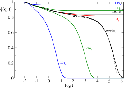
Figure 5: Coherent scattering functions, $\phi(q,t)$, as a function of time, $t$, in 3D (cf. Fig. 4) for a different wave number $q=7/2a$. The critical amplitude for $2qa=7$ is $h_{q}=0.367$. The von Schweidler law is shown dashed for a fitted time scale $\tau=1.21\times 10^{5}$.

The MCT equations of motion are known to admit scaling solutions at densities close to the critical density $\varphi_{c}(\varepsilon=1)$ Götze (2009). As the granular mode coupling equations are formally identical to those for an equilibrium hard sphere fluid, the scaling analysis is also closely related. To keep the presentation self contained, we will summarize the main results of this analysis. The analogous analysis for the incoherent scattering function discussed below in Sec. V was presented in II.

At small distances $\sigma(\varepsilon):=[\varphi_{c}(\varepsilon)-\varphi]/\varphi_{c}(\varepsilon)$ to the critical point, one finds

$$\phi(q,t;\sigma)=f_{q}^{c}+h_{q}G_{\sigma}(t),$$ (34)

where $h_{q}=h_{q}(\varepsilon)$ is the critical amplitude and $G_{\sigma}(t)$ is a scaling function, independent of the wave number. The scaling function $G_{\sigma}(t)$ can be characterized by a hierarchy of time scales. The shortest time scale is naturally provided by the mean time between collisions, $t_{0}\equiv\omega_{c}^{-1}$. The time scale $t_{\sigma}$ for the transition through the plateau, where $\phi(q,t_{\sigma};\sigma)=f_{q}^{c}$, diverges at the glass transition as $t_{\sigma}\propto\sigma^{-\delta}$ where $\delta=1/2a$. For short but macroscopic times, in the $\beta$-regime, one finds

$$G_{\sigma}(t)\propto(t/t_{0})^{-a},\quad t_{0}\ll t\leq t_{\sigma}.$$ (35a)

For larger times, $$t\geq t_{\sigma} \alpha \tau$$ but still well below the so called -relaxation time scale

$$G_{\sigma}(t)\propto-(t/t_{\sigma})^{b},\quad t_{\sigma}\leq t\ll\tau.$$ (35b)

Finally, for the largest times the time-density superposition principle holds, i.e., the coherent scattering functions can be collapsed on a master curve

$$\phi(q,t;\sigma)=\tilde{\phi}(q,t/\tau(q;\sigma)).$$ (36)

The time scale $\tau$ diverges at the glass transition, $\tau=\tau(q;\sigma)\propto\sigma^{-\gamma}$ where $\gamma=(1/2a)+(1/2b)$. An empirical choice for the scaling function $\tilde{\phi}(q,t)$ is provided by the Kohlrausch-Williams-Watts law $\tilde{\phi}_{\mathrm{KWW}}(q,t)\propto\exp(-t^{\beta})$ Williams and Watts (1970), crossing over to an exponential decay for the longest times Fuchs (1994).

The critical exponents $a,b$ in Eqs. (35) are related to a single exponent parameter $\lambda=\lambda(D,\varepsilon)$ by the universal relation

$$\lambda=\frac{\Gamma^{2}(1-a)}{\Gamma(1-2a)}=\frac{\Gamma^{2}(1+b)}{\Gamma(1+2b)},$$ (37)

where $\Gamma(x)$ is the Euler-Gamma-function.

Figure 6: Complete set of exponents in 3D as function of the coefficient of restitution $\varepsilon$. The top panel shows the exponents $\delta$ and $\gamma$ for the divergence of the time scales. The lower panel shows the exponents $a$ and $b$ for the master functions and the exponent parameter $\lambda$.

Figure 7: Complete set of exponents in 2D as function of the coefficient of restitution $\varepsilon$. The top panel shows the exponents $\delta$ and $\gamma$ for the divergence of the time scales. The lower panel shows the exponents $a$ and $b$ for the master functions and the exponent parameter $\lambda$.

The sets of exponents shown in Figs. 6 and 7 in 3D and 2D, respectively, are functions of the dimension but differ only slightly between $D=2$ and $D=3$. Overall, there is a tendency for the exponents in Figs. 6 and 7 to show slightly lesser stretching for higher dissipation, i.e. smaller $\varepsilon$. This may be interpreted as that the more dissipative and also more strongly driven fluid experiences less distinctive features in its glassy dynamics. The divergence in time scales is also expected to be a bit less pronounced. While the predicted changes in exponents are most likely hard to detect in experiments and simulation as absolute numbers, one should be able to detect the changes in comparison of different degrees of dissipation. Especially, the master functions should be comparably sensitive to changes in the exponents $a$ and $b$.

It is seen in Fig. 8 that for smaller $\varepsilon$ the order parameter $f_{q}^{c}$ decays more slowly for large wave numbers indicating a tighter localization. In comparison to 3D, the transition in 2D exhibits individually sharper peaks and overall a tighter localization for the same dissipation, cf. Fig. 9. It has been shown for data from simulation Sperl (2003) and experiments in colloidal suspensions van Megen (1995); Bayer et al. (2007), that the MCT predictions for the $f_{q}^{c}$ are typically accurate to around 20%. Hence, rather than fitting individual $f_{q}^{c}$ directly to measurements and numerical calculations, experimental and simulation data can be expected to follow the distributions shown on the 20%-level and exhibit trends with variation of $\varepsilon$ as indicated here.

It is seen in Fig. 4, that the critical law can only be observed without corrections for states closer than 0.1% to the transition point. Also, the von Schweidler law in Fig. 5 is only valid for an intermediate regime after the plateau. The regimes of applicability for the asymptotic scaling laws are therefore similar to the elastic case, and corrections to scaling are expected to follow the known trends Franosch et al. (1997).

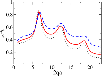
Figure 8: Critical glass-form factors $f_{q}^{c}$ at the transition for $\varepsilon=1.0$ (dotted curve), 0.5 (full curve) and 0.0 (dashed curve) in 2D.

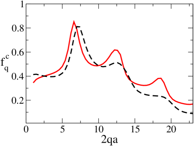
Figure 9: Critical glass-form factors $f_{q}^{c}$ at the respective transition points for $\varepsilon=0.5$ in 2D (full curve) and 3D (dashed curves).

V Tagged Particle Dynamics

The results of granular MCT for the tagged particle dynamics has been discussed in II. Here, we will focus on the derivation of the MCT equations.

The incoherent scattering function, $\phi_{s}(q,t)$, captures the tagged particle dynamics. This includes the mean square displacement $\delta r^{2}(t)=\left\langle[\bm{r}_{s}-\bm{r}_{s}(t)]^{2}\right\rangle$ which appears as an expansion coefficient of the incoherent scattering function $\phi_{s}(q,t)=1-q^{2}\delta r^{2}(t)/6+\mathcal{O}(q^{4})$ and the diffusivity $6D_{\infty}=\lim_{t\to\infty}\delta r^{2}(t)/t$ Boon and Yip (1992).

V.1 Equation of Motion

Following the reasoning that one should account for the conserved quantities and only for the conserved quantities explicitly, one would assume that the equation of motion for a tagged particle should be first order in time. The density $\rho_{s}$ being the only conserved quantity as the momentum of the tagged particle is all but conserved. It has been shown, though, that a consistent treatment of the tagged particle dynamics in fact requires an equation of motion which is second order in time Cichocki and Hess (1987); Pitts and Andersen (2000), thus effectively reintroducing the tagged particle momentum as a macroscopic observable.

We follow that reasoning and introduce the projector

$$\mathcal{P}_{s}=\sum_{\bm{q}}\left|\rho_{\bm{q}}^{s}\right\rangle\left\langle\rho_{\bm{q}}^{s}\right|+\sum_{\bm{q}}\left|j_{\bm{q}}^{sL}\right\rangle\left\langle j_{\bm{q}}^{sL}\right|/T.$$ (38)

Together with the microscopic state $\bm{a}_{\bm{q}}^{s}=(\rho_{\bm{q}}^{s},j_{\bm{q}}^{sL}/\sqrt{T})$, it yields an equation of motion for $\phi_{s}(q,t)$, formally identical to Eq. (16),

$$\ddot{\phi}_{s}(q,t) +\nu_{q}\dot{\phi}_{s}(q,t)+\Omega_{s}^{s}\phi_{s}(q,t)$$ (39)

$$+\Omega_{s}^{2}\int_{0}^{t}\!d\tau\,m_{s}(q,t-\tau)\dot{\phi}_{s}(q,\tau)$$

$$+\Omega_{s}^{2}\int_{0}^{t}\!d\tau\,L_{s}(q,t-\tau)\phi_{s}(q,\tau)=0,$$

with $\dot{\phi}_{s}(q,t=0)=0$ and $\phi_{s}(q,t=0)=1$. Moreover, $\Omega^{s}_{j\rho}=\left\langle j_{\bm{q}}^{sL}|\mathcal{L}_{+}\rho_{\bm{q}}^{s}\right\rangle/\sqrt{T}=q\sqrt{T}$ and $\Omega^{s}_{\rho j}=q\sqrt{T}$ do not depend on the coefficient of restitution as shown in appendix B.4. Hence, $\Omega_{s}^{2}:=\Omega^{s}_{j\rho}\Omega^{s}_{\rho j}=q^{2}T$ is identical to the corresponding quantity of the molecular fluid. This implies that looking at the probability density of the tagged particle on macroscopic time and length scales at very low densities, such that the memory kernel can be neglected, the microscopically broken time reversal symmetry is unobservable.

The memory kernels are given by

$$m_{s}(q,t) =\left\langle F_{\bm{q}}^{s\dagger}\tilde{\mathsf{U}}(t)F_{\bm{q}}^{s}\right\rangle/q^{2}T^{2},$$ (40a)

$$L_{s}(q,t) =\left\langle J_{\bm{q}}^{s\dagger}\tilde{\mathsf{U}}(t)F_{\bm{q}}^{s}\right\rangle/qT,$$ (40b)

with the fluctuating forces $F_{\bm{q}}^{s}=\mathcal{Q}_{s}\mathcal{L}_{+}j_{\bm{q}}^{sL}$ and $F_{\bm{q}}^{s\dagger}=\mathcal{Q}_{s}\mathcal{L}_{+}^{\dagger}j_{\bm{q}}^{sL}$ and the fluctuating current is $J_{\bm{q}}^{s\dagger}=\mathcal{Q}_{s}\mathcal{L}_{+}^{\dagger}\rho_{\bm{q}}^{s}$.

V.2 The Mode Coupling Approximation

We introduce a projection operator to describe the coupling between the tagged particle and the host fluid

$$\mathcal{P}_{2}^{s}=N\sum_{\bm{k},\bm{p}}\left|\rho_{\bm{k}}\rho^{s}_{\bm{p}}\right\rangle\left\langle\rho_{\bm{k}}\rho_{\bm{p}}^{s}\right|/S_{k}.$$ (41)

The corresponding mode coupling approximation reads

$$\tilde{\mathsf{U}}(t) \approx\mathcal{P}_{2}^{s}\tilde{\mathsf{U}}(t)\mathcal{P}_{2}^{s}$$ (42)

$$\approx N\sum_{\bm{k},\bm{p}}\left|\rho_{\bm{k}}\rho^{s}_{\bm{p}}\right\rangle\phi(k,t)\phi_{s}(p,t)\left\langle\rho_{\bm{k}}\rho^{s}_{\bm{p}}\right|/S_{k}.$$

Within the MCA we find that $L_{s}(q,t)=0$ and

$$m_{s}[\phi,\phi_{s}](q,t)\approx\\ \frac{1}{q^{2}T^{2}}\sum_{\bm{k},\bm{p}}\mathcal{V}_{\bm{q}\bm{k}\bm{p}}^{s}\mathcal{W}_{\bm{q}\bm{k}\bm{p}}^{s}\phi(k,t)\phi_{s}(p,t),$$ (43)

where

$$\mathcal{V}_{\bm{q}\bm{k}\bm{p}}^{s} =\sqrt{N/S_{k}}\left\langle j_{\bm{q}}^{sL}|\mathcal{L}_{+}\mathcal{Q}_{s}\rho_{\bm{k}}\rho_{\bm{p}}^{s}\right\rangle,$$ (44a)

$$\mathcal{W}_{\bm{q}\bm{k}\bm{p}}^{s} =\sqrt{N/S_{k}}\left\langle\rho_{\bm{k}}\rho_{\bm{p}}^{s}|\mathcal{Q}_{s}\mathcal{L}_{+}j_{\bm{q}}^{sL}\right\rangle.$$ (44b)

Here,

$$\mathcal{V}^{s}_{\bm{q}\bm{k}\bm{p}}=\frac{T}{\sqrt{NS_{k}}}(\hat{\bm{q}}\cdot\bm{k})(S_{k}-1)\delta_{\bm{q},\bm{k}+\bm{p}},$$ (45a)

is known from the literature Wahnström and Sjögren (1982); Bengtzelius et al. (1984) and one finds (cf. appendix B.6)

$$\mathcal{W}^{s}_{\bm{q}\bm{k}\bm{p}}=\frac{1+\varepsilon}{2}\frac{T}{\sqrt{NS_{k}}}(\hat{\bm{q}}\cdot\bm{k})(S_{k}-1)\delta_{\bm{q},\bm{k}+\bm{p}}.$$ (45b)

For the vertices, the loss of detailed balance reappears also for the tagged particle dynamics.

Together, Eqs. (45a) and (45b) yield

$$m_{s}[\phi,\phi_{s}](q,t)\approx\\ \frac{1+\varepsilon}{2}\frac{n}{q^{2}}\!\int d^{D}\!k\,S_{k}(\hat{\bm{q}}\cdot\bm{k})^{2}c_{k}^{2}\phi(k,t)\phi_{s}(|\bm{q}-\bm{k}|,t).$$ (46)

V.3 The approximate equation of motion

Finally, the equation of motion for the incoherent scattering function reads

$$\ddot{\phi}_{s}(q,t)+\nu_{q}\dot{\phi}_{s}(q,t)+\Omega_{s}^{2}\phi_{s}(q,t)\\ +\Omega_{s}^{2}\int_{0}^{\infty}\!d\tau\,m_{s}[\phi,\phi_{s}](q,t-\tau)\dot{\phi}_{s}(q,\tau)=0,$$ (47)

capturing the coupling of the tagged particle dynamics to the dynamics of the host fluid as reported in II.

The tagged particle is enslaved to the host fluid on macroscopic time scales. Consequently, it also develops persistent correlations, $f_{q}^{s}=\lim_{t\to\infty}\phi_{s}(q,t)$, at the critical density $\varphi_{c}$. They can be calculated from the equation

$$\frac{f_{q}^{s}}{1-f_{q}^{s}}=m[f,f^{s}](q).$$ (48)

A detailed discussion of the solutions of Eqs. (47,48) was given in II.

VI Discussion

The granular MCT, which includes and extends MCT for elastic hard spheres, shows that the dynamics of a driven granular fluid is for one remarkably similar to the equilibrium dynamics and at the same time fundamentally different. It is similar in that there is always a glass transition, accompanied by the two step relaxation scenario of dynamic correlation functions and diverging time scales. As both the order parameter $f_{q}(\varepsilon)$ and especially the critical exponents $a(\varepsilon)$ and $b(\varepsilon)$ depend on the coefficient of restitution $\varepsilon$, already slightly dissipative interactions ($\varepsilon\lesssim 1$) destroy the universality of the dynamics on long time scales, which is observed in elastic systems with either Newtonian or Brownian dynamics (I, Löwen et al., 1991; Gleim et al., 1998). The change of $\varepsilon$ will be detectable even on macroscopic time scales, in particular by observing the exponent $b(\varepsilon)$. This shows that the combination of dissipative collisions and driving cannot be mapped to an effective elastic hard sphere system with an effective temperature $T_{\mathrm{eff}}$, conceivably different from the granular temperature, $T$. Such a mapping, would allow to find a scaling function such that $\phi(q,t;\varepsilon)=\tilde{\phi}(q,t/t_{0}(\varepsilon))$.

The phase diagram in the $(T,\varphi)$-plane is still an open problem. The jamming density is defined for athermal ($T=0$) systems, while the granular glass transition is independent of temperature but assumes a finite temperature $T>0$ to sustain a fluid phase. It is not obvious, if and how they are connected. Our results suggest that the glass transition density, $\varphi_{c}$, is always strictly smaller than the quasi static jamming density $\varphi_{J}$. However, MCT is known to underestimate $\varphi_{c}$. What happens for densities $\varphi\geq\varphi_{c}(\varepsilon)$ larger than the critical density? At the glass transition, the $\alpha$-relaxation rate $\tau^{-1}$ diverges. Consequently, in every compression protocol using a small but finite compression rate, at some density the compression rate will be larger than the $\alpha$-relaxation rate $\tau^{-1}$. From then on, the evolution of the system will be restricted to a subset of phase space. The packings, which are reached from that subset by further compression will also be restricted to a subset of all packings and that might not even include those of highest density. Even if the ideal glass transition is destroyed by processes which are ignored within MCT, the enormous increase of relaxation times will be prohibitive for all practical purpose.

Apart from the Enskog term, Eqs. (19a,19b), the equations of motion are formally identical in two and three space dimensions. Hence the glass transition is qualitatively similar in two and three dimensions, with however different values for the critical density and the critical exponents. Compared to $D=3$, the glass from factors, $f_{q}$, decay slower in reciprocal space for $D=2$, indicating a stronger localization in two space dimensions.

In the final equations of motion, Eqs. (32) and (47), the driving force $\bm{\xi}$ appears only implicitly. While driving is crucial to achieve a stationary state, beyond that it does not alter the relaxation rates $\Omega_{ab},\Omega_{ab}^{s}$ and does not enter into the couplings to densities. Driving contributions would appear in the linear theory, if the (kinetic) energy, i.e., the granular temperature was included as a dynamic field. However this is hard to justify in a granular fluid, where kinetic energy is dissipated locally and hence not a hydrodynamic variable. In terms of the MCT, a coupling to the currents in $\mathcal{P}_{2}$ [Eq. (23)] would include explicit driving terms. Such a coupling was considered in the original mode coupling approaches Mazenko (1974); Sjögren (1980), but it’s relevance even in equilibrium fluids remains unclear.

VII Conclusion and Outlook

We considered randomly driven inelastic smooth hard disks (in $D=2$) and spheres (in $D=3$). We systematically derived equations of motion for the coherent scattering function, $\phi(q,t)$, and the incoherent scattering function, $\phi_{s}(q,t)$.

The equations of motion are formally identical to the ones for elastic hard sphere or disk fluids in thermal equilibrium but acquire a nontrivial dependence on the coefficient of restitution, $\varepsilon$. A transition to a glassy state, indicated by a nonzero value of the order parameter, $f_{q}$, appears through the bifurcation scenario of mode coupling theory. Like in thermal equilibrium, the spatial dimension of the system only enters via the static structure factors. In both dimensions, the critical packing fraction increases the more dissipative the particles are.

The dynamics around the plateau in the scattering functions is described by power laws with exponents, that are functions of the coefficient of restitution, $\varepsilon$. Together with the $\varepsilon$-dependence of the order parameter, $f_{q}$, this shows that the dynamics fundamentally changes upon varying the coefficient of restitution. In contrast, the difference between Newtonian and Brownian dynamics in thermal equilibrium, can be absorbed in the redefinition of the microscopic time scale. Also, a reduced long wavelength speed of sound is predicted for granular fluids.

One can hardly expect to observe a glass transition in a fluid of monodisperse hard spheres, because the system would quickly crystallize. To slow down crystal nucleation, usually binary mixtures with a small size difference are used Zaccarelli et al. (2009). For fluids in thermal equilibrium, it was found that a MCT for mixtures does not yield results that differ drastically from those for the monodisperse idealization Barrat and Latz (1990). For mixtures of granular particles, a new complication will be the non-equipartition of energy between the mixture species Barrat and Trizac (2002); Uecker et al. (2009).

So far we only derived equations for the correlation functions of spontaneous fluctuations. In a fluid in thermal equilibrium, this immediately entails knowledge about the corresponding response functions via the fluctuation dissipation theorem (FDT) de Groot and Mazur (1984). In fact, a lot of the experimental measurements are concerned with response spectra Jäckle (1986). The existence and form of a generalized FDT in driven granular fluids and more generally in systems far from equilibrium is a subject of active research Marconi et al. (2008).

It would certainly be desirable to weaken the assumptions made on the stationary phase space distribution function $\varrho(\Gamma)$. So far, we ignore correlations between the velocities of different particles which are known to be present in driven granular fluids Pagonabarraga et al. (2001). In light of the fact, that the single particle velocity distribution function is well represented by a simple Gaussian, these correlations can presumably be neglected as a first approximation. More serious are the static correlations, such as $S(q)$, which are known from simulations to differ from their elastic counterparts used here. However, we can easily incorporate data for the simulated structure factors into our approach; work along these lines is in progress.

The results presented above deal with a specific, highly idealized system. It is a natural question to ask how robust these results are qualitatively. No qualitative changes are expected for a speed dependent coefficient of restitution $\varepsilon=\varepsilon(v)$. Also models that can be described by an effective coefficient of restitution Schäfer et al. (1996) like, e.g., the spring-dashpot model are expected to show a nonequilibrium glass transition. The inclusion of inter-particle friction or the treatment of different driving forces will likely pose a number of challenges. Such changes might lead to equations of motion and results qualitatively different from the ones discussed here.

Appendix A The Granular Yvon-Born-Green Relation

The Yvon-Born-Green (YBG) relation between the pair- and the triplet correlation function follows from the identity

$$\nabla_{1}g(r_{12}) =(\varrho^{-1}\nabla_{12}\varrho)g(r_{12})$$ (49)

$$+n\int d^{D}r_{3}\,g_{3}(\bm{r}_{1},\bm{r}_{2},\bm{r}_{3})(\varrho^{-1}\nabla_{13}\varrho),$$

where $\varrho^{-1}$ is the pseudo-inverse of the distribution function Born and Green (1946). For elastic hard spheres, where $\varrho(\Gamma)\propto\prod_{i<j}\Theta(r_{ij}-2a)$ This yields the known relation Hansen and McDonald (2006)

$$\nabla_{1}g(r_{12}) =\hat{\bm{r}}_{12}\delta(r_{12}-2a)g(r_{12})$$ (50)

$$+n\int d^{D}r_{3}\,\hat{\bm{r}}_{13}\delta(r_{13}-2a)g_{3}(\bm{r}_{1},\bm{r}_{2},\bm{r}_{3}).$$

For the inelastic hard spheres, there must be an additional spatial dependence of the distribution function, depending on the coefficient of restitution, $\varepsilon$, or otherwise, e.g., the structure factor $S_{q}$ would not depend on $\varepsilon$.

Overlapping configurations still have zero probability and because of homogeneity, only relative distances play a role. Therefor, the distribution function will be of the form $\varrho(\Gamma)\propto\prod_{i<j}\Theta(r_{ij}-2a)\vartheta_{\varepsilon}(r_{ij})$ with a unknown function $\vartheta_{\varepsilon}(r)>0$. With this, we get a granular hard sphere YBG relation

$$\nabla_{1}g(r_{12}) =\hat{\bm{r}}_{12}\delta(r_{12}-2a)g(r_{12})+g(r_{12})\nabla_{1}\ln\vartheta_{\varepsilon}(r_{12})$$

$$+n\int d^{D}r_{3}\,\hat{\bm{r}}_{13}\delta(r_{13}-2a)g_{3}(\bm{r}_{1},\bm{r}_{2},\bm{r}_{3})$$

$$+n\int d^{D}r_{3}\,g_{3}(\bm{r}_{1},\bm{r}_{2},\bm{r}_{3})\nabla_{1}\ln\vartheta_{\varepsilon}(r_{13}).$$

Unfortunately, virtually nothing is known about the function $\vartheta_{\varepsilon}(r)$. Therefor we use the elastic hard sphere YBG relation which means we make the nontrivial approximation

$$g(r_{12})\nabla_{1}\ln\vartheta_{\varepsilon}(r_{12})\\ \approx-n\int d^{D}r_{3}\,g_{3}(\bm{r}_{1},\bm{r}_{2},\bm{r}_{3})\nabla_{1}\ln\vartheta_{\varepsilon}(r_{13})$$ (51)

which may be more general than setting $\vartheta_{\varepsilon}(r)\equiv 1$.

On the next level, we have

$$\nabla_{1}g_{3}(123) =[\hat{\bm{r}}_{12}\delta(r_{12}-2a)+\hat{\bm{r}}_{13}\delta(r_{13}-2a)]g_{3}(123)$$

$$+g_{3}(123)\nabla_{1}[\ln\vartheta_{\varepsilon}(r_{12})+\ln\vartheta_{\varepsilon}(r_{13})]$$

$$+n\int d^{D}r_{4}\,\hat{\bm{r}}_{14}\delta(r_{14}-2a)g_{4}(1234)$$

$$+n\int d^{D}r_{4}\,g_{4}(1234)\nabla_{1}\ln\vartheta_{\varepsilon}(r_{14})$$

using the abbreviation $i\equiv\bm{r}_{i}$. In Eq. (73) below, we use the approximation

$$g_{3}(123)\nabla_{1}[\ln\vartheta_{\varepsilon}(r_{12})+\ln\vartheta_{\varepsilon}(r_{13})]\\ \approx-n\int d^{D}r_{4}\,g_{4}(1234)\nabla_{1}\ln\vartheta_{\varepsilon}(r_{14})$$ (52)

Appendix B Matrix Elements

B.1 The Frequency $\Omega_{jj}$ in Two Dimensions

We have to determine

$$\left\langle j_{\bm{q}}^{L}|\mathcal{L}_{+}j_{\bm{q}}^{L}\right\rangle=i\frac{N(N-1)}{2}\left\langle j_{\bm{q}}^{L}|\mathcal{T}_{12}^{+}j_{\bm{q}}^{L}\right\rangle$$ (53)

where all other contributions vanish due to parity. Explicitly, this reads

$$\left\langle j_{\bm{q}}^{L}|\mathcal{L}_{+}j_{\bm{q}}^{L}\right\rangle=\frac{1+\varepsilon}{2}i\left\langle(\hat{\bm{q}}\cdot\bm{v}_{1})(\hat{\bm{q}}\cdot\hat{\bm{r}}_{12})(\hat{\bm{r}}_{12}\cdot\bm{v}_{12})^{2}\Theta(-\hat{\bm{r}}_{12}\cdot\bm{v}_{12})\delta(r_{12}-2a)\big{(}e^{i\bm{q}\cdot\bm{r}_{12}}-1\big{)}\right\rangle,$$ (54)

where the three particle term vanishes, again, due to parity. Introducing the relative velocity $\bm{v}:=(\bm{v}_{1}-\bm{v}_{2})/\sqrt{2}$, the velocity averages can be evaluated

$$\left\langle(\hat{\bm{q}}\cdot\bm{v}_{1})(\hat{\bm{r}}_{12}\cdot\bm{v}_{12})^{2}\Theta(-\hat{\bm{r}}_{12}\cdot\bm{v}_{12})\right\rangle =\sqrt{2}(\hat{\bm{q}}\cdot\hat{\bm{r}}_{12})\left\langle(\hat{\bm{r}}_{12}\cdot\bm{v}_{12})^{3}\Theta(-\hat{\bm{r}}_{12}\cdot\bm{v}_{12})\right\rangle$$ (55)

$$=\frac{\sqrt{2}}{2\pi T}(\hat{\bm{q}}\cdot\hat{\bm{r}}_{12})\int_{0}^{\infty}\!dv\int_{\pi/2}^{3\pi/2}\!d\varphi\,v^{4}\cos^{3}\varphi e^{-v^{2}/2T}$$

$$=-2T\sqrt{T/\pi}(\hat{\bm{q}}\cdot\hat{\bm{r}}_{12}).$$

The remaining spatial average reads

$$\left\langle(\hat{\bm{q}}\cdot\hat{\bm{r}}_{12})^{2}\delta(r_{12}-2a)\big{(}e^{i\bm{q}\cdot\bm{r}_{12}}-1\big{)}\right\rangle\\ =-\frac{2a\chi}{V}\int_{0}^{2\pi}d\varphi\,\cos^{2}\varphi\big{(}1-e^{2iaq\cos\varphi}\big{)}.$$ (56)

One finds

$$\frac{1}{\pi}\int_{0}^{2\pi}d\varphi\,\cos^{2}\varphi e^{iz\cos\varphi}=-2\frac{d^{2}J_{0}(z)}{dz^{2}},$$ (57)

i.e.,

$$\left\langle(\hat{\bm{q}}\cdot\hat{\bm{r}}_{12})^{2}\delta(r_{12}-2a)\big{(}e^{i\bm{q}\cdot\bm{r}_{12}}-1\big{)}\right\rangle\\ =-\frac{2\pi na\chi}{N}[1+2J_{0}^{\prime\prime}(2aq)].$$ (58)

Collecting terms, one arrives at Eq. (19a).

B.2 The Frequency $\Omega_{\rho j}$

The driving contribution vanishes and the free streaming contribution yields

$$\left\langle\rho_{\bm{q}}|\mathcal{L}_{0}j_{\bm{q}}^{L}\right\rangle =\frac{q}{N^{2}}\left\langle\sum_{j,k}(\hat{\bm{q}}\cdot\bm{v}_{k})^{2}e^{-i\bm{q}\cdot\bm{r}_{jk}}\right\rangle$$ (59)

$$=qTS_{q}/N.$$

The collisional contribution reads

$$\frac{N(N-1)}{2}\left\langle\rho_{\bm{q}}|\mathcal{T}_{12}j_{\bm{q}}^{L}\right\rangle=\frac{1+\varepsilon}{4}\hat{\bm{q}}\cdot\left\langle(\hat{\bm{r}}_{12}\cdot\bm{v}_{12})^{2}\hat{\bm{r}}_{12}\Theta(-\hat{\bm{r}}_{12}\cdot\bm{v}_{12})\delta(r_{12}-2a)\big{(}e^{i\bm{q}\cdot\bm{r}_{2}}-e^{i\bm{q}\cdot\bm{r}_{1}}\big{)}\sum\nolimits_{j}e^{-i\bm{q}\cdot\bm{r}_{j}}\right\rangle.$$ (60)

The velocity integration yields a factor $T/2$ while the spatial average can be rewritten as

$$\left\langle\hat{\bm{r}}_{12}\delta(r_{12}-2a)\big{(}e^{i\bm{q}\cdot\bm{r}_{2}}-e^{i\bm{q}\cdot\bm{r}_{1}}\big{)}\sum\nolimits_{j}e^{-i\bm{q}\cdot\bm{r}_{j}}\right\rangle\\ =2\left\langle\hat{\bm{r}}_{12}\delta(r_{12}-2a)e^{-i\bm{q}\cdot\bm{r}_{12}}\right\rangle\\ +2(N-2)\left\langle\hat{\bm{r}}_{12}\delta(r_{12}-2a)e^{-i\bm{q}\cdot\bm{r}_{3}}e^{i\bm{q}\cdot\bm{r}_{2}}\right\rangle.$$ (61)

Application of the YBG relation to the second term yields

$$N\left\langle\hat{\bm{r}}_{12}\delta(r_{12}-2a)e^{-i\bm{q}\cdot\bm{r}_{3}}e^{i\bm{q}\cdot\bm{r}_{2}}\right\rangle\\ =-\frac{1}{N}(S_{q}-1)-\left\langle\hat{\bm{r}}_{12}\delta(r_{12}-2a)e^{-i\bm{q}\cdot\bm{r}_{12}}\right\rangle,$$ (62)

i.e., the second term in Eq. (62) cancels the first term in Eq. (61). Combining the remaining terms we arrive at Eq. (20b).

B.3 The Vertex $\mathcal{W}_{\bm{q}\bm{k}\bm{p}}$

As the vertex is linear in $\bm{v}_{i}$, there is no contribution from the driving, $i\mathcal{L}_{D}^{+}$. Expanding the projector $\mathcal{Q}_{c}$, the vertex reads

$$\mathcal{W}_{\bm{q}\bm{k}\bm{p}}=N\left\langle\rho_{\bm{k}}\rho_{\bm{p}}|\mathcal{L}_{+}j_{\bm{q}}^{L}\right\rangle/S_{p}\\ -N^{2}\left\langle\rho_{\bm{k}}\rho_{\bm{p}}|\rho_{\bm{q}}\right\rangle\left\langle\rho_{\bm{q}}|\mathcal{L}_{+}j_{\bm{q}}^{L}\right\rangle/S_{p}S_{q}.$$ (63)

The free streaming contribution to the first term is given by

$$\left\langle\rho_{\bm{k}}\rho_{\bm{p}}|\mathcal{L}_{0}j_{\bm{q}}^{L}\right\rangle =qT\left\langle\rho_{\bm{k}}\rho_{\bm{p}}|\rho_{\bm{q}}\right\rangle$$ (64)

$$=\frac{qT}{N^{2}}\delta_{\bm{k}+\bm{p},\bm{q}}S^{(3)}(\bm{k},\bm{p}).$$

For the collisional contribution we find

$$\frac{N(N-1)}{2}\left\langle\rho_{\bm{k}}\rho_{\bm{p}}|\mathcal{T}_{12}^{+}j_{\bm{q}}^{L}\right\rangle=i\frac{1+\varepsilon}{4N}T\hat{\bm{q}}\cdot\left\langle\sum_{j,k}e^{-i\bm{k}\cdot\bm{r}_{j}}e^{-i\bm{p}\cdot\bm{r}_{k}}\hat{\bm{r}}_{12}\delta(r_{12}-2a)\big{(}e^{i\bm{q}\cdot\bm{r}_{2}}-e^{i\bm{q}\cdot\bm{r}_{1}}\big{)}\right\rangle$$ (65)

The average on the right hand side shall be abbreviated as $\left\langle jk|12\right\rangle$. Then this can be expanded as

$$\left\langle jk|12\right\rangle=\left\langle 11|12\right\rangle+\left\langle 22|12\right\rangle+\left\langle 12|12\right\rangle+\left\langle 21|12\right\rangle\\ +N(\left\langle 13|12\right\rangle+\left\langle 23|12\right\rangle+\left\langle 31|12\right\rangle+\left\langle 32|12\right\rangle)\\ +N\left\langle 33|12\right\rangle+N^{2}\left\langle 34|12\right\rangle$$ (66)

Exploiting the symmetries, this can be simplified to

$$\left\langle jk|12\right\rangle=2\left\langle 11|12\right\rangle+\left\langle 12|12\right\rangle+2N\left\langle 13|12\right\rangle\\ +N\left\langle 33|12\right\rangle+N^{2}\left\langle 34|12\right\rangle$$ (67)

Proceeding term by term we first find

$$\left\langle 11|12\right\rangle=\left\langle e^{i(\bm{k}+\bm{p}-\bm{q})\cdot\bm{r}_{1}}\hat{\bm{r}}_{12}\delta(r_{12}-2a)\big{(}e^{i\bm{q}\cdot\bm{r}_{12}}-1\big{)}\right\rangle$$

which can be reduced to

$$\left\langle 11|12\right\rangle =\delta_{\bm{k}+\bm{p},\bm{q}}\left\langle\hat{\bm{r}}_{12}\delta(r_{12}-2a)e^{i\bm{q}\cdot\bm{r}_{12}}\right\rangle$$ (68)

$$\equiv\delta_{\bm{k}+\bm{p},\bm{q}}\bm{G}(\bm{q}).$$

The second term can be reduced to an equivalent expression

$$\left\langle 12|12\right\rangle =\left\langle e^{i(\bm{k}+\bm{p}-\bm{q})\cdot\bm{r}_{1}}\hat{\bm{r}}_{12}\delta(r_{12}-2a)e^{i\bm{q}\cdot\bm{r}_{12}}\right\rangle$$

$$-\left\langle e^{i(\bm{k}+\bm{p}-\bm{q})\cdot\bm{r}_{1}}\hat{\bm{r}}_{12}\delta(r_{12}-2a)e^{i(\bm{k}-\bm{q})\cdot\bm{r}_{12}}\right\rangle,$$

i.e.,

$$\left\langle 12|12\right\rangle=\delta_{\bm{k}+\bm{p},\bm{q}}[\bm{G}(\bm{k})+\bm{G}(\bm{p})].$$ (69)

The first three particle term

$$\left\langle 13|12\right\rangle =\left\langle e^{i(\bm{k}+\bm{p}-\bm{q})\cdot\bm{r}_{2}}e^{i\bm{k}\cdot\bm{r}_{12}}e^{i\bm{p}\cdot\bm{r}_{32}}\hat{\bm{r}}_{12}\delta(r_{12}-2a)\right\rangle$$

$$-\left\langle e^{i(\bm{k}-\bm{q})\cdot\bm{r}_{1}}e^{i\bm{p}\cdot\bm{r}_{3}}\hat{\bm{r}}_{12}\delta(r_{12}-2a)\right\rangle$$

requires a little more work. The first term shall be abbreviated as

$$\left\langle e^{i(\bm{k}+\bm{p}-\bm{q})\cdot\bm{r}_{2}}e^{i\bm{k}\cdot\bm{r}_{12}}e^{i\bm{p}\cdot\bm{r}_{32}}\hat{\bm{r}}_{12}\delta(r_{12}-2a)\right\rangle\\ =\delta_{\bm{k}+\bm{p},\bm{q}}\bm{H}(\bm{k},\bm{p}).$$ (70)

The second term can be simplified with the help of the YBG relation

$$\left\langle e^{i(\bm{k}-\bm{q})\cdot\bm{r}_{1}}e^{i\bm{p}\cdot\bm{r}_{3}}\hat{\bm{r}}_{12}\delta(r_{12}-2a)\right\rangle\\ =\frac{1}{N^{2}}\delta_{\bm{k}+\bm{p},\bm{q}}[i\bm{p}(S_{p}-1)+N\bm{G}(\bm{p})].$$ (71)

Similarly, the second three particle term

$$\left\langle 33|12\right\rangle=\left\langle e^{i(\bm{k}+\bm{p})\cdot\bm{r}_{3}}\hat{\bm{r}}_{12}\delta(r_{12}-2a)\big{(}e^{-i\bm{q}\cdot\bm{r}_{2}}-e^{-i\bm{q}\cdot\bm{r}_{1}}\big{)}\right\rangle$$

can be reduced by employing the YBG relation

$$\left\langle 33|12\right\rangle=-\frac{2}{N^{2}}\delta_{\bm{k}+\bm{p},\bm{q}}[i\bm{q}(S_{q}-1)+N\bm{G}(\bm{q})].$$ (72)

The four particle term

$$\left\langle 34|12\right\rangle=\left\langle e^{i\bm{k}\cdot\bm{r}_{3}}e^{i\bm{p}\cdot\bm{r}_{4}}\hat{\bm{r}}_{12}\delta(r_{12}-2a)\big{(}e^{-i\bm{q}\cdot\bm{r}_{2}}-e^{-i\bm{q}\cdot\bm{r}_{1}}\big{)}\right\rangle$$

is naturally the most involved. Using the higher order YBG relation it reads

$$\left\langle 34|12\right\rangle= -\frac{2}{NV^{3}}\int d^{D}r_{2}d^{D}r_{3}d^{D}r_{4}\,e^{-i\bm{q}\cdot\bm{r}_{2}}e^{i\bm{k}\cdot\bm{r}_{3}}e^{i\bm{p}\cdot\bm{r}_{4}}\frac{\partial}{\partial\bm{r}_{2}}g_{3}(\bm{r}_{2},\bm{r}_{3},\bm{r}_{4})$$ (73)

$$+\frac{2}{NV^{3}}\int d^{D}r_{2}d^{D}r_{3}d^{D}r_{4}\,e^{-i\bm{q}\cdot\bm{r}_{2}}e^{i\bm{k}\cdot\bm{r}_{3}}e^{i\bm{p}\cdot\bm{r}_{4}}\hat{\bm{r}}_{23}\delta(r_{23}-2a)g_{3}(\bm{r}_{2},\bm{r}_{3},\bm{r}_{4})$$

$$+\frac{2}{NV^{3}}\int d^{D}r_{2}d^{D}r_{3}d^{D}r_{4}\,e^{-i\bm{q}\cdot\bm{r}_{2}}e^{i\bm{k}\cdot\bm{r}_{3}}e^{i\bm{p}\cdot\bm{r}_{4}}\hat{\bm{r}}_{24}\delta(r_{24}-2a)g_{3}(\bm{r}_{2},\bm{r}_{3},\bm{r}_{4}).$$

Partial integration in the first term and the extraction of the momentum conservation constraint yields

$$\left\langle 34|12\right\rangle= -\frac{2i\bm{q}}{NV^{2}}\delta_{\bm{k}+\bm{p},\bm{q}}\int d^{D}r_{23}d^{D}r_{24}\,e^{-i\bm{k}\cdot\bm{r}_{23}}e^{-i\bm{p}\cdot\bm{r}_{24}}g_{3}(\bm{r}_{23},\bm{r}_{24})$$ (74)

$$+\frac{2}{NV^{2}}\delta_{\bm{k}+\bm{p},\bm{q}}\int d^{D}r_{23}d^{D}r_{24}\,e^{-i\bm{k}\cdot\bm{r}_{23}}e^{-i\bm{p}\cdot\bm{r}_{24}}g_{3}(\bm{r}_{23},\bm{r}_{24})\hat{\bm{r}}_{23}\delta(r_{23}-2a)$$

$$+\frac{2}{NV^{2}}\delta_{\bm{k}+\bm{p},\bm{q}}\int d^{D}r_{23}d^{D}r_{24}\,e^{-i\bm{k}\cdot\bm{r}_{23}}e^{-i\bm{p}\cdot\bm{r}_{24}}g_{3}(\bm{r}_{23},\bm{r}_{24})\hat{\bm{r}}_{24}\delta(r_{24}-2a).$$

This leaves us with the relatively simple expression

$$\left\langle 34|12\right\rangle= -\frac{2i\bm{q}}{N^{3}}\delta_{\bm{k}+\bm{p},\bm{q}}[S^{(3)}(\bm{k},\bm{p})-S_{k}-S_{p}-S_{q}+2]$$

$$-\frac{2}{N}\delta_{\bm{k}+\bm{p},\bm{q}}[\bm{H}(\bm{k},\bm{p})+\bm{H}(\bm{p},\bm{k})].$$

Most terms cancel to yield

$$\left\langle jk|12\right\rangle=\frac{2i}{N}\delta_{\bm{k}+\bm{p},\bm{q}}[\bm{k}S_{p}+\bm{p}S_{k}-\bm{q}S^{(3)}(\bm{k},\bm{p})]$$ (75)

or

$$\frac{N(N-1)}{2}\left\langle\rho_{\bm{k}}\rho_{\bm{p}}|\mathcal{T}_{12}^{+}j_{\bm{q}}^{L}\right\rangle\\ =-\frac{1+\varepsilon}{2}\frac{T}{N^{2}}[(\hat{\bm{q}}\cdot\bm{k})S_{p}+(\hat{\bm{q}}\cdot\bm{p})S_{k}-qS^{(3)}(\bm{k},\bm{p})].$$ (76)

Inserting Eq. (64) and Eq. (76) into Eq. (63) and applying the convolution approximation yields Eq. (29b).

B.4 The Frequency $\Omega_{\rho j}^{s}$

The free streaming contribution reads

$$\left\langle\rho_{\bm{q}}^{s}|\mathcal{L}_{0}j_{\bm{q}}^{sL}\right\rangle=q\left\langle(\hat{\bm{q}}\cdot\bm{v}_{s})^{2}\right\rangle=qT$$ (77)

and the collisional contribution

$$(N-1)\left\langle\rho_{\bm{q}}^{s}\mathcal{T}_{1s}^{+}j_{\bm{q}}^{sL}\right\rangle=i\frac{1+\varepsilon}{2}N\left\langle(\hat{\bm{r}}_{1s}\cdot\bm{v}_{1s})^{2}(\hat{\bm{q}}\cdot\hat{\bm{r}}_{1s})\Theta(-\hat{\bm{r}}_{1s}\cdot\bm{v}_{1s})\delta(r_{1s}-2a)\right\rangle=0$$ (78)

vanishes due to symmetry.

B.5 The Vertex $\mathcal{V}_{\bm{q}\bm{k}\bm{p}}^{s}$

The left incoherent vertex is given as

$$\mathcal{V}_{\bm{q}\bm{k}\bm{p}}^{s}=\left\langle j_{\bm{q}}^{sL}|\mathcal{L}_{+}\rho_{\bm{k}}\rho_{\bm{p}}^{s}\right\rangle-\left\langle j_{\bm{q}}^{sL}|\mathcal{L}_{+}\rho_{\bm{q}}^{s}\right\rangle\left\langle\rho_{\bm{q}}^{s}|\rho_{\bm{k}}\rho_{\bm{p}}^{s}\right\rangle.$$ (79)

The triple density correlator,

$$\left\langle\rho_{\bm{q}}^{s}|\rho_{\bm{k}}\rho_{\bm{p}}^{s}\right\rangle=\frac{1}{N}\delta_{\bm{k}+\bm{p},\bm{q}}S_{k},$$ (80)

is related to the structure factor. Moreover, we have

$$\left\langle j_{\bm{q}}^{sL}|\mathcal{L}_{+}\rho_{\bm{k}}\rho_{\bm{p}}^{s}\right\rangle=k\left\langle j_{\bm{q}}^{sL}|j_{\bm{k}}^{L}\rho_{\bm{p}}^{s}\right\rangle+p\left\langle j_{\bm{q}}^{sL}|\rho_{\bm{k}}j_{\bm{p}}^{sL}\right\rangle$$ (81)

as only the free streaming operator $i\mathcal{L}_{0}$ applies. The velocity integration yield a factor of T

$$\left\langle j_{\bm{q}}^{sL}|\mathcal{L}_{+}\rho_{\bm{k}}\rho_{\bm{p}}^{s}\right\rangle =\frac{kT}{N}\left\langle\rho_{\bm{q}}^{s}|\rho_{\bm{k}}^{s}\rho_{\bm{p}}^{s}\right\rangle+pT\left\langle\rho_{\bm{q}}^{s}|\rho_{\bm{k}}\rho_{\bm{p}}^{s}\right\rangle$$ (82)

$$=\frac{1}{N}[(\hat{\bm{q}}\cdot\bm{k})T+(\hat{\bm{q}}\cdot\bm{p})S_{k}]\delta_{\bm{k}+\bm{p},\bm{q}}.$$

Collecting terms one arrives at Eq. (45a).

B.6 The Vertex $\mathcal{W}_{\bm{q}\bm{k}\bm{p}}^{s}$

The incoherent vertex is given as

$$\mathcal{W}_{\bm{q}\bm{k}\bm{p}}^{s}=\left\langle\rho_{\bm{k}}\rho_{\bm{p}}^{s}|\mathcal{L}_{+}j_{\bm{q}}^{sL}\right\rangle-\left\langle\rho_{\bm{k}}\rho_{\bm{p}}^{s}|\rho_{\bm{q}}^{s}\right\rangle\left\langle\rho_{\bm{q}}^{s}|\mathcal{L}_{+}j_{\bm{q}}^{sL}\right\rangle.$$ (83)

The free streaming contribution is simple

$$\left\langle\rho_{\bm{k}}\rho_{\bm{p}}^{s}|\mathcal{L}_{0}j_{\bm{q}}^{sL}\right\rangle=qT\left\langle\rho_{\bm{k}}\rho_{\bm{p}}^{s}|\rho_{\bm{q}}^{s}\right\rangle=\frac{qT}{N}\delta_{\bm{k}+\bm{p},\bm{q}}S_{k}.$$ (84)

For the collisional part one finds with the velocity integration being already performed

$$(N-1)\left\langle\rho_{\bm{k}}\rho_{\bm{p}}^{s}|\mathcal{T}_{1s}^{+}j_{\bm{q}}^{sL}\right\rangle =i\frac{1+\varepsilon}{2}\frac{T}{N}\left\langle\sum\nolimits_{j}e^{-i\bm{k}\cdot\bm{r}_{j}}e^{-i(\bm{p}-\bm{q})\cdot\bm{r}_{s}}(\hat{\bm{q}}\cdot\bm{r}_{1s})\delta(r_{1s}-2a)\right\rangle$$ (85)

$$=i\frac{1+\varepsilon}{2}\frac{T}{N}\delta_{\bm{k}+\bm{p}-\bm{q}}\left\langle\sum\nolimits_{j}e^{-i\bm{k}\cdot\bm{r}_{js}}(\hat{\bm{q}}\cdot\bm{r}_{1s})\delta(r_{1s}-2a)\right\rangle.$$

The spatial average,

$$\left\langle\sum\nolimits_{j}e^{-i\bm{k}\cdot\bm{r}_{js}}(\hat{\bm{q}}\cdot\bm{r}_{1s})\delta(r_{1s}-2a)\right\rangle=\left\langle e^{-i\bm{k}\cdot\bm{r}_{1s}}(\hat{\bm{q}}\cdot\bm{r}_{1s})\delta(r_{1s}-2a)\right\rangle+N\left\langle e^{-i\bm{k}\cdot\bm{r}_{2s}}(\hat{\bm{q}}\cdot\bm{r}_{1s})\delta(r_{1s}-2a)\right\rangle,$$ (86)

can again be evaluated with the help of the YBG relation. Applying it to the second term cancels the first term and we get

$$(N-1)\left\langle\rho_{\bm{k}}\rho_{\bm{p}}^{s}|\mathcal{T}_{1s}^{+}j_{\bm{q}}^{sL}\right\rangle\\ =\frac{1+\varepsilon}{2}\frac{T}{N}\delta_{\bm{k}+\bm{p}-\bm{q}}(\hat{\bm{q}}\cdot\bm{k})(S_{k}-1).$$ (87)

Collecting terms one arrives at Eq. (45b).

Appendix C Details of the Numerics

For the numerical solution of Eqs. (32,33,47), we used well established algorithms in 3D Franosch et al. (1997) and 2D Bayer et al. (2007). Reciprocal space is discretized into $M^{3}$ grid points ($M=100$) up to a cutoff of $2qa=40$ in 3D, and with $M=125$ up a cutoff of 2qa = 50 in 2D. The time axis is also discrete with a grid of $N=2048$ points and a step size that is doubled in successive steps to accommodate for logarithmic time scales. The initial time step is $\Delta t=10^{-9}t_{0}$. The critical density $\varphi_{c}$ is located by interval bisection.

References

- Greer (1995) A. L. Greer, Science 267, 1947 (1995).
- van Megen (1995) W. van Megen, Transp. Theory Stat. Phys. 24, 1017 (1995).
- Höhler and Cohen-Addad (2005) R. Höhler and S. Cohen-Addad, J. Phys.: Condens. Matt. 17, R1041 (2005).
- Marty and Dauchot (2005) G. Marty and O. Dauchot, Phys. Rev. Lett. 94, 015701 (2005).
- Abate and Durian (2006) A. R. Abate and D. J. Durian, Phys. Rev. E 74, 031308 (2006).
- Goldman and Swinney (2006) D. I. Goldman and H. L. Swinney, Phys. Rev. Lett. 96, 145702 (2006).
- Reis et al. (2007) P. M. Reis, R. A. Ingale, and M. D. Shattuck, Phys. Rev. Lett. 98, 188301 (2007).
- Keys et al. (2007) A. S. Keys, A. R. Abate, S. C. Glotzer, and D. J. Durian, Nature physics 3, 260 (2007).
- Kranz et al. (2010) W. T. Kranz, M. Sperl, and A. Zippelius, Phys. Rev. Lett. 104, 225701 (2010).
- Sperl et al. (2012) M. Sperl, W. T. Kranz, and A. Zippelius, EPL 98, 28001 (2012).
- Pusey and van Megen (1986) P. N. Pusey and W. van Megen, Nature 320, 340 (1986).
- Debenedetti and Stillinger (2001) P. G. Debenedetti and F. H. Stillinger, Nature 410, 259 (2001).
- Cavagna (2009) A. Cavagna, Phys. Rep. 476, 51 (2009).
- Götze (2009) W. Götze, Complex dynamics of glass-forming liquids: a mode-coupling theory (Oxford University Press, USA, 2009).
- Fuchs and Cates (2002) M. Fuchs and M. E. Cates, Phys. Rev. Lett. 89, 248304 (2002).
- Fuchs and Cates (2009) M. Fuchs and M. E. Cates, J. Rheol. 53, 957 (2009).
- Habdas et al. (2004) A. Habdas, D. Schaar, A. Levitt, and E. Weeks, Europhys. Lett. 67, 477 (2004).
- Gazuz et al. (2009) I. Gazuz, A. Puertas, T. Voigtmann, and M. Fuchs, Phys. Rev. Lett. 102, 248302 (2009).
- Candelier and Dauchot (2009) R. Candelier and O. Dauchot, Phys. Rev. Lett. 103, 128001 (2009).
- Cates et al. (1998) M. E. Cates, J. P. Wittmer, J.-P. Bouchaud, and P. Claudin, Phys. Rev. Lett. 81, 1841 (1998).
- Pica Ciamarra et al. (2010) M. Pica Ciamarra, M. Nicodemi, and A. Coniglio, Soft Matter 6, 2871 (2010).
- Liu and Nagel (1998) A. J. Liu and S. R. Nagel, Nature 396, 21 (1998).
- O’Hern et al. (2003) C. S. O’Hern, L. E. Silbert, A. J. Liu, and S. R. Nagel, Phys. Rev. E 68, 011306 (2003).
- Iverson (1997) R. M. Iverson, Rev. Geophys. 35, 245 (1997).
- Prevost et al. (2002) A. Prevost, D. A. Egolf, and J. S. Urbach, Phys. Rev. Lett. 89, 084301 (2002).
- Aranson and Olafsen (2002) I. S. Aranson and J. S. Olafsen, Phys. Rev. E 66, 061302 (2002).
- Kohlstedt et al. (2005) K. Kohlstedt, A. Snezhko, M. V. Sapozhnikov, I. S. Aranson, J. S. Olafsen, and E. Ben-Naim, Phys. Rev. Lett. 95, 068001 (2005).
- Maaß et al. (2008) C. C. Maaß, N. Isert, G. Maret, and C. M. Aegerter, Phys. Rev. Lett. 100, 248001 (2008).
- Ojha et al. (2004) R. P. Ojha, P. A. Lemieux, P. K. Dixon, A. J. Liu, and D. J. Durian, Nature 427, 521 (2004).
- Abate and Durian (2005) A. R. Abate and D. J. Durian, Phys. Rev. E 72, 031305 (2005).
- Schröter et al. (2005) M. Schröter, D. I. Goldman, and H. L. Swinney, Phys. Rev. E 71, 030301 (2005).
- Haff (1983) P. K. Haff, J. Fluid Mech. 134, 401 (1983).
- McNamara (1993) S. McNamara, Phys. Fluids A 5, 3056 (1993).
- Goldhirsch and Zanetti (1993) I. Goldhirsch and G. Zanetti, Phys. Rev. Lett. 70, 1619 (1993).
- Altenberger (1975) A. R. Altenberger, Physica A 80, 46 (1975).
- Aspelmeier et al. (2001) T. Aspelmeier, M. Huthmann, and A. Zippelius, in Granular Gases, edited by T. Pöschel and S. Luding (Springer, 2001) pp. 31–58.
- Note (1) This is just an unusual rendering of Itō’s Lemma Øksendal (2003).
- Ernst et al. (1969) M. H. Ernst, J. R. Dorfmann, W. R. Hoegy, and J. M. J. van Leeuwen, Physica 45, 127 (1969).
- Note (2) We use the convention .
- Mori (1965) H. Mori, Prog. Theor. Phys. 34, 399 (1965).
- Brout (1959) R. Brout, Phys. Rev. 115, 824 (1959).
- Percus and Yevick (1958) J. K. Percus and G. J. Yevick, Phys. Rev. 110, 1 (1958).
- Ashcroft and Lekner (1966) N. W. Ashcroft and J. Lekner, Phys. Rev. 145, 83 (1966).
- Carnahan and Starling (1969) N. F. Carnahan and K. E. Starling, J. Chem. Phys. 51, 635 (1969).
- Baus and Colot (1987) M. Baus and J. L. Colot, Phys. Rev. A 1, 3912 (1987).
- Jeffrey and Zwillinger (2000) A. Jeffrey and D. Zwillinger, eds., Gradshteyn and Ryzhik’s Table of Integrals, Series, and Products, 6th ed. (Academic Press, 2000).
- Leutheusser (1982) E. Leutheusser, J. Phys. C 15, 2801 (1982).
- Note (3) A factor of was missing in I & II. This has no influence on the results discussed there.
- Hansen and McDonald (2006) J.-P. Hansen and I. R. McDonald, Theory of Simple Liquids, 3rd ed. (Academic Press, 2006).
- Schweizer and Curro (1988) K. S. Schweizer and J. G. Curro, Phys. Rev. Lett. 60, 809 (1988).
- Boon and Yip (1992) J. P. Boon and S. Yip, Molecular Hydrodynamics (Dover Publications, 1992).
- van Noije et al. (1999) T. P. C. van Noije, M. H. Ernst, E. Trizac, and I. Pagonabarraga, Phys. Rev. E 59, 4326 (1999).
- Fixman (1962) M. Fixman, J. Chem. Phys. 36, 310 (1962).
- Kawasaki (1966) K. Kawasaki, Phys. Rev. 150, 291 (1966).
- Kadanoff and Swift (1968) L. P. Kadanoff and J. Swift, Phys. Rev. 166, 89 (1968).
- Bosse et al. (1978) J. Bosse, W. Götze, and M. Lücke, Phys. Rev. A 17, 434 (1978).
- Barrat et al. (1989) J. L. Barrat, W. Götze, and A. Latz, J. Phys.: Condens. Matter 1, 7163 (1989).
- Jackson and Feenberg (1962) H. W. Jackson and E. Feenberg, Rev. Mod. Phys. 34 (1962).
- Franosch et al. (1997) T. Franosch, M. Fuchs, W. Götze, M. R. Mayr, and A. P. Singh, Phys. Rev. E 55, 7153 (1997).
- Williams and Watts (1970) G. Williams and D. C. Watts, Trans. Faraday Soc. 66, 80 (1970).
- Fuchs (1994) M. Fuchs, J. Non-Cryst. Solids 172, 241 (1994).
- Sperl (2003) M. Sperl, Phys. Rev. E 68, 031405 (2003).
- Bayer et al. (2007) M. Bayer, J. Brader, F. Ebert, M. Fuchs, E. Lange, G. Maret, R. Schilling, M. Sperl, and J. Wittmer, Phys. Rev. E 76, 011508 (2007).
- Cichocki and Hess (1987) B. Cichocki and W. Hess, Physica. A 141, 475 (1987).
- Pitts and Andersen (2000) S. J. Pitts and H. C. Andersen, J. Chem. Phys. 113, 3945 (2000).
- Wahnström and Sjögren (1982) G. Wahnström and L. Sjögren, J. Phys. C 15, 401 (1982).
- Bengtzelius et al. (1984) U. Bengtzelius, W. Götze, and A. Sjölander, J. Phys. C 17, 5915 (1984).
- Note (4) We are not aware of a published derivation within the projection operator formalism, though. We present it in appendix B.5.
- Löwen et al. (1991) H. Löwen, J.-P. Hansen, and J.-N. Roux, Phys. Rev. A 44, 1169 (1991).
- Gleim et al. (1998) T. Gleim, W. Kob, and K. Binder, Phys. Rev. Lett. 81, 4404 (1998).
- Mazenko (1974) G. F. Mazenko, Phys. Rev. A 9, 360 (1974).
- Sjögren (1980) L. Sjögren, Phys. Rev. A 22, 2866 (1980).
- Zaccarelli et al. (2009) E. Zaccarelli, C. Valeriani, E. Sanz, W. C. K. Poon, M. E. Cates, and P. N. Pusey, Phys. Rev. Lett. 103, 135704 (2009).
- Barrat and Latz (1990) J. L. Barrat and A. Latz, J. Phys.: Condens. Matt. 2, 4289 (1990).
- Barrat and Trizac (2002) A. Barrat and E. Trizac, Granular Matter 4, 57 (2002).
- Uecker et al. (2009) H. Uecker, W. T. Kranz, T. Aspelmeier, and A. Zippelius, Phys. Rev. E 80, 041303 (2009).
- de Groot and Mazur (1984) S. R. de Groot and P. Mazur, Non-equilibrum Thermodynamics (Dover Publications, Inc., New York, 1984).
- Jäckle (1986) J. Jäckle, Rep. Prog. Phys. 49, 171 (1986).
- Marconi et al. (2008) U. M. B. Marconi, A. Puglisi, L. Rondoni, and A. Vulpiani, Phys. Rep. 461, 111 (2008).
- Pagonabarraga et al. (2001) I. Pagonabarraga, E. Trizac, T. P. C. van Noije, and M. H. Ernst, Phys. Rev. E 65, 011303 (2001).
- Schäfer et al. (1996) J. Schäfer, S. Dippel, and D. E. Wolf, J. Phys. I 6, 5 (1996).
- Born and Green (1946) M. Born and H. S. Green, Proc. R. Soc. A 188, 10 (1946).
- Øksendal (2003) B. K. Øksendal, Stochastic differential equations: an introduction with applications (Springer Verlag, 2003).