Boundary perturbations and the Helmholtz equation in three dimensions

Abstract

We propose an analytic perturbative scheme for determining the eigenvalues of the Helmholtz equation, $(\nabla^{2}+k^{2})\psi=0$, in three dimensions with an arbitrary boundary where $\psi$ satisfies either the Dirichlet boundary condition ($\psi=0$ on the boundary) or the Neumann boundary condition (the normal gradient of $\psi$, $\frac{\partial\psi}{\partial n}$ is vanishing on the boundary). Although numerous works are available in the literature for arbitrary boundaries in two dimensions, to best of our knowledge the formulation in three dimensions is proposed for the first time. In this novel prescription, we have expanded the arbitrary boundary in terms of spherical harmonics about an equivalent sphere and obtained perturbative closed-form solutions at each order for the problem in terms of corrections to the equivalent spherical boundary for both the boundary conditions. This formulation is in parallel with the standard time-independent Rayleigh-Schrödinger perturbation theory. The efficiency of the method is tested by comparing the perturbative values against the numerically calculated eigenvalues for spheroidal, superegg and superquadric shaped boundaries. It is shown that this perturbation works quite well even for wide departure from spherical shape and for higher excited states too. We believe this formulation would find applications in the field of quantum dots and acoustical cavities.

I Introduction

A recent experiment has reported that the geometry of nanoscale second-phase particles are superellipsoids in nature [1]. A good estimation of the energyspectra of these geometries may help us to explore the shape of these particles more accurately. For estimation of energyspectra of these nanoscale particles one needs to solve the Helmholtz equation in three dimensions (3D) with arbitrary boundaries. This is the main concern of this note and we believe, it is the first instance when an analytic perturbative formulation has been proposed to solve the Helmholtz equation for arbitrary shaped boundaries in 3D.
The Helmholtz equation is one of the ubiquitous partial differential equations in physics as well as in engineering. It appears in different realms of physical and engineering problems across diverse fields - like the study of membrane vibration, eigenanalysis in acoustic cavities, electromagnetic wave propagation (TE/TM modes) in a waveguide and quantum mechanics. Most of these problems have been pursued in order to find out the energy eigenvalues/eigenfrequencies of the linear homogeneous Helmholtz equation subjected to different boundary conditions and various geometries in two or three dimensions. In the classical scenario, standard wave equation reduces to the Helmholtz equation for the sinusoidal time dependence. Also, in the quantum manifestation, the unitary evolution of wavefunction will transform the Schrödinger equation into the equation of our interest. Canonical examples of boundary conditions are either Dirichlet boundary condition (DBC) where the eigenfunction vanishes on the boundary or Neumann boundary condition (NBC) where the normal gradient of the eigenfunction becomes zero on the boundary. Of the above mentioned problems, the cases of membrane vibrations, propagation of the TM modes within a waveguide and confinement of a quantum particle in potential well fall under the DBC umbrella and the case of transmission of TE modes through waveguides and acoustic cavities are the prominent examples of NBC. To classify the solutions of Helmholtz equation according to the nature of boundary condition and also as per the shape of the boundary is an intricate task. Analytic closed form solutions to these problems are available only for a restricted class of boundary geometries. The problems for rectangular, circular, elliptical and triangular (equilateral and right angled isosceles) boundaries are examples of such limited class in two dimensions [2]. For Helmholtz equation in three dimensions there are $11$ such `special' separable co-ordinate systems where the solution can be written as a product of three factors each of which are dependent on only one co-ordinate [3]. The beautiful property of these family of separated solutions is that the linear combination of these solutions will eventually give us all solutions of the Helmholtz equation. Even in these restricted class most of the solutions have multi-parameter dependence and which makes them difficult to use. But, in most physical problems, one comes across boundaries for which one of more coordinates are constant not frozen in any of those `special' co-ordinate systems. Explicit solutions are available in the literature only for spherical, rectangular and cylindrical enclosures [4, 5]. In this context, finding solutions of the Helmholtz equation for any arbitrary shaped boundary becomes a dreadful job.
Recently the two dimensional version of this problem has been investigated extensively in both the direction - analytical [6, 7, 8, 9, 10, 11] as well as numerical [12, 13, 14, 15, 16, 17]. But for the three dimensional case such an analytic closed form solution by means of perturbation is not yet addressed. There are a few attempts made in this direction via numerical means in the context of chaos in general 3D billiard [18, 19, 20, 21, 22, 23] and also some exciting experiments to investigate wave chaos in microwave cavities [24] and in resonant optical cavities [25]. In this paper we address the problem of solving the Helmholtz equations in 3D for simply connected arbitrary shaped boundaries. In this method, an arbitrary boundary has been approximated as a perturbation about a sphere of `average radius' and expanded in terms of the spherical harmonics with a deformation parameter sitting in front of them. The next task is to improve upon the `average radius' approximation by incorporating the correction terms arising due to the boundary perturbation. So, we expand the wavefunction and energy eigenvalues in a standard perturbative series and collect terms of different orders to get the respective governing equations. In a similar fashion we rewrite the boundary conditions for different orders. We then calculate the energy and wavefunction corrections for degenerate and non-degenerate states for both the cases of boundary condition separately. Finally we have compared our analytic results against the numerical values for spheroid, superegg and superquadric shapes and it has been shown that the analytic values agree quite well with the numerical ones for small departures from the sphere. The formulation is seen to work very well even for large deviations from sphere. To justify the previous statement, we have calculated the low lying spectra for an octahedron and a cube by perturbing a sphere and matched them with the numerically calculated and exactly known results respectively.
The paper is organised as follows: The section II prescribes the general scheme in abstract sense. In section III, we apply these prescriptions to the case of spheroids, supereggs and superquadrics. A short conclusion and a few comments close the final section.

II Formulation

The homogeneous Helmholtz equation on a three dimensional flat simply connected volume $\cal T$ is given by,

$$\left(\nabla^{2}+k^{2}\right)\psi\equiv\left(\nabla^{2}+E\right)\psi=0,$$ (1)

where $\nabla^{2}$ is the Laplacian operator in 3D. We are interested in finding out the eigenspectrum in the interior of the bounded region for the case of Dirichlet and Neumann condition on the surface $\partial{\cal T}$. The parameter $k^{2}$ is obtained by applying the Dirichlet boundary condition and can always be matched with $E$, the energy of a quantum particle confined in the above mentioned region. In this case, the function $\psi$ would be identified as the wavefunction of the particle. Whereas for example, in the case of acoustical enclosure one would apply the Neumann boundary condition on $\psi$, which is nothing but a velocity potential and values of $k\leavevmode\nobreak\ (=\sqrt{E})$ would determine the pitch of the eigenmodes or the resonating frequencies. For the two dimensional case of a vibrating membrane it was shown by Rayleigh [2] that : ``the gravest tone of a membrane, whose boundary is approximately circular, is nearly the same as that of a mechanically similar membrane in the form of a circle of the same mean radius or area.'' In the same spirit of the two dimensional case, we have developed a formalism to calculate the eigenspectrum of an arbitrary shaped enclosure by perturbing about a sphere of `mean radius'. In Appendix A.1 and A.2, we have extended the Rayleigh's result for three dimensions and justify the perturbation around the `mean radius'.

It is natural to work in the spherical polar coordinate system $(r,\theta,\phi)$, where any closed surface satisfies the periodic condition $r(\theta,\phi+2\pi)=r(\theta,\phi)$. Now, we choose an arbitrary closed surface of the form $r=r(\theta,\phi)$ as the boundary of our problem. The first step is to construct a sphere of `mean radius' $R_{0}$ which is given by

$$R_{0}=\frac{1}{4\pi}\int\limits_{0}^{\pi}\int\limits_{0}^{2\pi}r(\theta,\phi)\sin\theta\,{\rm d}\theta{\rm d}\phi\,.$$ (2)

The next step is to expand the given arbitrary shape as a perturbation over the spherical surface of `mean radius' $R_{0}$ in terms of the spherical harmonics of the following form

$$r(\theta,\phi)=R_{0}\left(1+\lambda\sum_{a=1}^{\infty}\sum_{b=-a}^{+a}C_{a}^{b}Y_{a}^{b}(\theta,\phi)\right)=R_{0}\left(1+\lambda f(\theta,\phi)\right)\,,$$ (3)

where

$$Y_{a}^{b}(\theta,\phi)=\sqrt{\frac{2a+1}{4\pi}}\sqrt{\frac{(a-b)!}{(a+b)!}}P_{a}^{b}(\cos\theta)\leavevmode\nobreak\ {\rm e}^{ib\phi}\,;\leavevmode\nobreak\ \leavevmode\nobreak\ Y_{a}^{-b}(\theta,\phi)=(-1)^{b}\leavevmode\nobreak\ \overline{Y_{a}^{b}(\theta,\phi)},$$ (4)

$$f(\theta,\phi)=\sum_{a=1}^{\infty}\sum_{b=-a}^{+a}C_{a}^{b}Y_{a}^{b}(\theta,\phi).$$ (5)

$Y_{a}^{b}$ is the spherical harmonics of order $a$ and degree $b$. $P_{a}^{b}$ is the associated Legendre polynomial of order $a$ and degree $b$ and $C_{a}^{b}$s are the expansion coefficients. Here, the spherical harmonics are chosen in such a manner that they are normalised to unity, i.e.

$$\int\limits_{0}^{\pi}\int\limits_{0}^{2\pi}\overline{Y_{a}^{b}(\theta,\phi)}Y_{c}^{d}(\theta,\phi)\sin\theta{\rm d}\theta{\rm d}\phi=\delta_{a,c}\delta_{b,d}.$$ (6)

The parameter $\lambda$ is a measure of the deformation, which in principle, should be small compared to unity in order to ensure the validation of the perturbation theory. However as we will observe in the following section that the perturbation works reasonably well for large deformation also. In the limit $\lambda\rightarrow 0$, $r(\theta,\phi)=R_{0}$, represents a sphere. We also note that the parameter $\lambda$ is an artificial one, which can be easily absorbed in the coefficient $C_{a}^{b}$. It is used here to keep track of the orders of perturbation. The missing term $C_{0}^{0}Y_{0}^{0}$ in the above expansion can always be absorbed in the definition of $R_{0}$ given by (3) in agreement with (2).

Now, as per first approximation, at the zeroth order level, the eigenvalue $E_{0}$ and the wavefunction $\psi_{0}$ of the system bounded by $r(\theta,\phi)$ will be given by that corresponding to the sphere of `mean radius' $R_{0}$

$$\psi_{0}(r,\theta,\phi)=\tilde{N}_{n,l}\leavevmode\nobreak\ j_{l}(kr)P_{l}^{m}(\cos\theta)e^{im\phi}=N_{n,l}\leavevmode\nobreak\ j_{l}(\rho)Y_{l}^{m}(\theta,\phi)\,,$$ (7)

$$E_{0}=\begin{cases}\beta_{n,l}^{2}/R_{0}^{2}&\mbox{for \leavevmode\nobreak\ DBC}\\ \alpha_{n,l}^{2}/R_{0}^{2}&\mbox{for\leavevmode\nobreak\ NBC}\end{cases}$$ (8)

where $\rho=kr$, $N_{n,l}$ is a suitable normalisation constant (which is independent of $m$) with $l\in\mathbb{N}$, $n\in\mathbb{N}_{>0}$, $m=\{-l,-(l-1),\cdots,0,\cdots,l-1,l\}\in\mathbb{Z}$ and $j_{l}(\rho)$ is $l^{\rm{th}}$ order spherical Bessel function. $\beta_{n,l}\,(=k_{n,l}R_{0})$ is the $n^{\rm{th}}$ node of the $l^{\rm{th}}$ order spherical Bessel function, i.e. $j_{l}(\beta_{n,l})=0$ and $\alpha_{n,l}\,(=k_{n,l}R_{0})$ is the $n^{\rm{th}}$ zero of the derivative of the $l^{\rm{th}}$ order spherical Bessel function, i.e. $j^{\prime}_{l}(\alpha_{n,l})=0$. The values of $\beta_{n,l}$ and $\alpha_{n,l}$ are distinct for different sets of $n$ and $l$. There is no repetition of $n$ values for a given value of $l$ but $m$ can have $(2l+1)$ values, so for $l=0$ the states are non-degenerate while for non-zero $l$ values the states are $(2l+1)$-fold degenerate.

Our next task is to improve upon the `mean radius' approximation by incorporating the correction terms arising due to the boundary perturbation. So, we will expand $\psi$ and $E$ as

$$\psi=\psi_{0}+\lambda\psi_{1}+\lambda^{2}\psi_{2}+\cdots\cdots\,,$$ (9)

$$E=E_{0}+\lambda E_{1}+\lambda^{2}E_{2}+\cdots\cdots\,,$$ (10)

where the zeroth order terms represent the wavefunction and the eigenvalue of the unperturbed state and rest of the terms are corrections of different orders to the wavefunction and the eigenvalue respectively. Substituting these expansions in (1) and collecting the coefficients of different powers of $\lambda$ from both the sides we obtained the following set of equations after some rearrangements

$$\mathcal{O}(\lambda^{0}):\qquad\qquad\leavevmode\nobreak\ \left(\nabla^{2}+E_{0}\right)\psi_{0}=0,$$ (11)

$$\mathcal{O}(\lambda^{1}):\qquad\qquad\leavevmode\nobreak\ \left(\nabla^{2}+E_{0}\right)\psi_{1}=-E_{1}\psi_{0},$$ (12)

$$\mathcal{O}(\lambda^{2}):\qquad\qquad\leavevmode\nobreak\ \left(\nabla^{2}+E_{0}\right)\psi_{2}=-E_{1}\psi_{1}-E_{2}\psi_{0}.$$ (13)

Eq. (11) can easily be identified as the equation for a particle confined in a spherical box with $\psi_{0}$ as the wavefunction corresponding to the eigenvalue $E_{0}$. Now, we will set up the formalism in a generic way for the degenerate and non-degenerate states for both the Dirichlet and the Neumann boundary conditions separately.

II.1 Boundary conditions

Like the governing equations the boundary conditions are written for different orders of perturbation for both the cases in the following.

II.1.1 Dirichlet boundary condition

The boundary condition is

$$\psi(r(\theta,\phi))=0.$$ (14)

Taylor expanding the above expression about $r=R_{0}$ using (3) and (9) one obtains the boundary condition at each order in the following form,

$$\mathcal{O}(\lambda^{0}):\qquad\leavevmode\nobreak\ \psi_{0}(R_{0},\theta,\phi)=0,$$ (15)

$$\mathcal{O}(\lambda^{1}):\qquad\leavevmode\nobreak\ \psi_{1}(R_{0},\theta,\phi)+\,R_{0}f(\theta,\phi)\psi_{0}^{\prime}(R_{0},\theta,\phi)=0,$$ (16)

$$\mathcal{O}(\lambda^{2}):\qquad\leavevmode\nobreak\ \psi_{2}(R_{0},\theta,\phi)+\,R_{0}f(\theta,\phi)\psi_{1}^{\prime}(R_{0},\theta,\phi)+\frac{R_{0}^{2}}{2}f^{2}(\theta,\phi)\psi_{0}^{\prime\prime}(R_{0},\theta,\phi)=0,$$ (17)

where

$$f(\theta,\phi)=\sum_{a=1}^{\infty}\sum_{b=-a}^{+a}C_{a}^{b}Y_{a}^{b}(\theta,\phi).$$ (18)

From now on the dependence of $Y_{a}^{b}$ (and $f$) and $\psi$s on the arguments $(\theta,\phi)$ and $(r,\theta,\phi)$ respectively is not shown explicitly for brevity. In the above expressions, prime ($\prime$) denotes partial differentiation with respect to $r$.

II.1.2 Neumann boundary condition

The Neumann boundary condition is given by

$${\bf\nabla{\psi}}\cdot{\bf n}=0\,,$$ (19)

where ${\bf n}$ is the normal at the boundary surface given by $r=r(\theta,\phi)$. Expanding (19) in the Taylor series about $r=R_{0}$ using (3) and (9), the conditions at different orders of $\lambda$ are obtained as follows,

$$\mathcal{O}(\lambda^{0}):\qquad\psi_{0}^{\prime}(R_{0})=0,$$ (20)

$$\mathcal{O}(\lambda^{1}):\qquad\psi_{1}^{\prime}(R_{0})+R_{0}f\psi_{0}^{\prime\prime}(R_{0})-\frac{1}{R_{0}}\hat{f}\hat{\psi_{0}}(R_{0})-\frac{1}{R_{0}\sin^{2}\theta}\check{f}\check{\psi_{0}}(R_{0})=0,$$ (21)

$$\mathcal{O}(\lambda^{2}):\qquad\psi_{2}^{\prime}(R_{0})+R_{0}f\psi_{1}^{\prime\prime}(R_{0})+\frac{1}{2}R_{0}^{2}f^{2}{\psi_{0}}^{\prime\prime\prime}(R_{0})-\frac{1}{R_{0}}\hat{f}\hat{\psi_{1}}(R_{0})$$

$$\qquad\qquad\qquad+\frac{2}{R_{0}}f\hat{f}\hat{\psi_{0}}(R_{0})-\frac{1}{R_{0}\sin^{2}\theta}\check{f}\check{\psi_{1}}(R_{0})+\frac{2}{R_{0}\sin^{2}\theta}f\check{f}\check{\psi_{0}}(R_{0})=0.$$ (22)

In the above expressions prime (^′), hat (${\bf\hat{\phantom{x}}}$) and check (${\bf\check{\phantom{x}}}$) denote partial differentiation with respect to $r$, $\theta$ and $\phi$ respectively. In the following we will discuss separately the non-degenerate and degenerate cases. Since, the governing equations are same for both the cases of DBC and NBC, the general solutions are same with differences only in the argument $\rho$, respective coefficients and normalisation constants which are dictated by the respective boundary condition.

II.2 Non-degenerate states ($l=0$)

II.2.1 Dirichlet boundary condition

For $l=0$ state we have,

$$\psi_{0}=\tilde{N}_{n,0}\leavevmode\nobreak\ j_{0}(\rho)Y_{0}^{0}\equiv N_{n,0}\leavevmode\nobreak\ j_{0}(\rho)\,,$$ (23)

where $\rho=(\beta_{n,0}/R_{0})r$, $j_{0}$ is the zeroth-order spherical Bessel function and $N_{n,0}=\tilde{N}_{n,0}Y_{0}^{0}=(2\pi R^{3}_{0}j^{2}_{1}(\beta_{n,0}))^{-\frac{1}{2}}$ is the normalisation constant. $E_{0}$ is obtained from (8) with $l=0$ and an appropriate value of $n$, as $\psi_{0}$ is constrained by the boundary condition (15).
The first order correction to the wavefunction is obtained by solving (12). Substituting the expression for $\psi_{0}$ from (23) into (12), the most general solution is given by

$$\psi_{1}=\sum_{p=1}^{\infty}\sum_{q=-p}^{+p}A_{p}^{q}j_{p}(\rho)Y_{p}^{q}+A_{0}^{0}Y^{0}_{0}j_{0}(\rho)-\frac{\rho E_{1}}{2E_{0}}N_{n,0}j_{1}(\rho).$$ (24)

The last term in the above solution is the particular integral to the differential equation (12) due to the inhomogeneity. Taking a hint from the two dimensional case [8, 10, 11] this specific closed form of the particular solution was inspected. Imposing the boundary condition (16) over $\psi_{1}$ and matching the coefficients of different orders of spherical harmonics, we obtain the first order eigenvalue correction (comparing the coefficient of $Y_{0}^{0}$) as well as the coefficients $A_{p}^{q}$ (comparing the coefficient of $Y_{p}^{q}$) of the following form

$$A_{p}^{q}=\rho_{0}N_{n,0}C_{p}^{q}\frac{j_{1}(\rho_{0})}{j_{p}(\rho_{0})};\qquad\rho_{0}\equiv\rho\rvert_{{}_{r=R_{0}}}=\beta_{n,0},$$ (25)

$$E_{1}=0.$$ (26)

The remaining constant $A_{0}^{0}$, which is not required for our present purpose, can be fixed by normalising the corrected eigenfunction over the entire volume $\cal T$. From (26) it is evident that any possible non-zero correction to the eigenvalue eigenvalue will come from higher orders.
The second order calculation will replicate that of the first order. Plugging the value of $E_{1}=0$ in (13) we obtained the second order correction to the wavefunction as

$$\psi_{2}=\sum_{p=1}^{\infty}\sum_{q=-p}^{+p}B_{p}^{q}j_{p}(\rho)Y_{p}^{q}+B_{0}^{0}Y^{0}_{0}j_{0}(\rho)-\frac{\rho E_{2}}{2E_{0}}N_{n,0}j_{1}(\rho).$$ (27)

Implementing the boundary condition (17) over $\psi_{2}$ we have estimated the second order correction to the eigenvalue by collecting the constant terms in (17), as

$$\frac{E_{2}}{E_{0}}=\sum\limits_{p=1}^{\infty}\sum\limits_{q=-p}^{p}\frac{(-1)^{q}}{2\pi}\leavevmode\nobreak\ C_{p}^{q}\leavevmode\nobreak\ C_{p}^{-q}\left(1+\frac{\rho_{0}j^{\prime}_{p}(\rho_{0})}{j_{p}(\rho_{0})}\right),$$ (28)

$$B_{p}^{q}=\frac{\rho_{0}j_{1}(\rho_{0})}{j_{p}(\rho_{0})}A_{0}^{0}Y_{0}^{0}C_{p}^{q}-\frac{N_{n,0}\rho_{0}j_{1}(\rho_{0})}{j_{p}(\rho_{0})}\sum_{a=1}^{\infty}\sum_{b=-a}^{+a}\sum^{a+p}\limits_{k=\left\lceil\begin{subarray}{c}|a-p|\\ |q-b|\end{subarray}\right\rceil}\sqrt{\frac{(2a+1)(2k+1)}{4\pi(2p+1)}}\leavevmode\nobreak\ C_{a}^{b}C_{k}^{q-b}$$

$$\qquad\times\langle ak00|p0\rangle\langle akb(q-b)|pq\rangle\left(1+\frac{\rho_{0}j^{\prime}_{a}(\rho_{0})}{j_{a}(\rho_{0})}\right),$$ (29)

where $\left\lceil\begin{subarray}{c}|a-p|\\ |q-b|\end{subarray}\right\rceil\equiv$ Maximum ($|a-p|,|q-b|$), $\rho_{0}$ is the same as defined earlier in (25) and $\langle n_{1}n_{2}m_{1}m_{2}|nm\rangle$ gives the Clebsch-Gordan coefficient for the decomposition of $|n_{1},n_{2},n,m\rangle$ in terms of $|n_{1},m_{1}\rangle$ $|n_{2},m_{2}\rangle$.The remaining constant $B_{0}^{0}$ can be extracted out by normalising the corrected wavefunction up to the second order. At each order, the corrections to the wavefunction and eigenvalue are expressed in a generic manner in terms of the expansion coefficients $C_{a}^{b}$ of the boundary perturbation. This formalism works for any type of closed surface which is slightly perturbed from a spherical one. So, for a given surface, we first need to calculate the `mean radius' $R_{0}$ and subsequently $C_{a}^{b}$s to estimate the second order correction to the eigenvalue.

II.2.2 Neumann boundary condition

For $l=0$ state we have,

$$\psi_{0}=\tilde{\bar{N}}_{n,0}\leavevmode\nobreak\ j_{0}(\rho)Y_{0}^{0}\equiv{\bar{N}_{n,0}}\leavevmode\nobreak\ j_{0}(\rho)\,,$$ (30)

where $\rho=(\alpha_{n,0}/R_{0})r$ and ${\bar{N}_{n,0}}=\tilde{\bar{N}}_{n,0}Y_{0}^{0}=(2\pi R^{3}_{0}j^{2}_{0}(\alpha_{n,0}))^{-\frac{1}{2}}$ is the normalisation constant. $E_{0}$ is obtained from (8) with $l=0$ and a given value of $n$.
Solution of (12) yields the first order correction to the wavefunction. Plugging $\psi_{0}$ into (12), we obtained the general solution, like the DBC case

$$\psi_{1}=\sum_{p=1}^{\infty}\sum_{q=-p}^{+p}\bar{A}_{p}^{q}j_{p}(\rho)Y_{p}^{q}+\bar{A}_{0}^{0}Y^{0}_{0}j_{0}(\rho)-\frac{\rho E_{1}}{2E_{0}}\bar{N}_{n,0}j_{1}(\rho).$$ (31)

Imposing the boundary condition (21) on $\psi_{1}$ we have obtained

$$\bar{A}_{p}^{q}=\bar{\rho}_{0}\bar{N}_{n,0}C_{p}^{q}\frac{j_{0}(\bar{\rho}_{0})}{j^{\prime}_{p}(\bar{\rho}_{0})};\qquad\bar{\rho}_{0}\equiv\rho\rvert_{{}_{r=R_{0}}}=\alpha_{n,0}\,,$$ (32)

$$E_{1}=0.$$ (33)

This establishes the 3D generalisation of 2D Rayleigh's theorem mentioned earlier, viz. ``tones of symmetric modes of an arbitrary shaped cavity which is not very elongated is very nearly equal to that of a sphere of the same mean radius''. The remaining constant $\bar{A}_{0}^{0}$ can be fixed by normalising the corrected eigenfunction over the entire volume $\cal T$.
Substituting the value of $E_{1}=0$ in (13) we obtained the second order correction to the wavefunction as

$$\psi_{2}=\sum_{p=1}^{\infty}\sum_{q=-p}^{+p}\bar{B}_{p}^{q}j_{p}(\rho)Y_{p}^{q}+\bar{B}_{0}^{0}Y^{0}_{0}j_{0}(\rho)-\frac{\rho E_{2}}{2E_{0}}\bar{N}_{n,0}j_{1}(\rho).$$ (34)

As $\psi_{2}$ is restricted by the boundary condition (22), we get the second order correction to the eigenvalue as

$$\frac{E_{2}}{E_{0}}=\sum\limits_{p=1}^{\infty}\sum\limits_{q=-p}^{p}\frac{(-1)^{q}}{2\pi}\leavevmode\nobreak\ C_{p}^{q}\leavevmode\nobreak\ C_{p}^{-q}\left(1+\frac{\bar{\rho}_{0}j_{p}(\bar{\rho}_{0})}{j^{\prime}_{p}(\bar{\rho}_{0})}\right),$$ (35)

$$\bar{B}_{p}^{q}=\frac{\bar{\rho}_{0}j_{0}(\bar{\rho}_{0})}{j^{\prime}_{p}(\bar{\rho}_{0})}\bar{A}_{0}^{0}Y_{0}^{0}C_{p}^{q}+\frac{\bar{N}_{n,0}\bar{\rho}_{0}j_{0}(\bar{\rho}_{0})}{j^{\prime}_{p}(\bar{\rho}_{0})}\sum_{a=1}^{\infty}\sum_{b=-a}^{+a}\sum^{a+p}\limits_{k=\left\lceil\begin{subarray}{c}|a-p|\\ |q-b|\end{subarray}\right\rceil}\sqrt{\frac{(2a+1)(2k+1)}{4\pi(2p+1)}}\leavevmode\nobreak\ C_{a}^{b}C_{k}^{q-b}$$

$$\times\langle ak00|p0\rangle\langle akb(q-b)|pq\rangle\left\{1+\frac{\bar{\rho}_{0}j_{a}(\bar{\rho}_{0})}{j^{\prime}_{a}(\bar{\rho}_{0})}+\frac{k(k+1)-a(a+1)-p(p+1)}{2\bar{\rho}_{0}}\frac{j_{a}(\bar{\rho}_{0})}{j^{\prime}_{a}(\bar{\rho}_{0})}\right\}.$$ (36)

By collecting the coefficients of $Y_{p}^{q}$ in (22) we have extracted out $\bar{B}_{p}^{q}$. However, these constants are required only for the calculation of higher order correction terms. The remaining constant $\bar{B}_{0}^{0}$ in $\psi_{2}$ can be obtained from the normalisation condition of the corrected wavefunction up to second order. We observe that these results are beautiful generalisations of our earlier work in two dimensions [11].

II.3 Degenerate case ($l\neq 0$)

II.3.1 Dirichlet boundary condition

For $l\neq$ 0 the wavefunction of the unperturbed state is given by

$$\psi_{0}=N_{n,l}\leavevmode\nobreak\ j_{l}(\rho)Y_{l}^{m},$$ (37)

where $N_{n,l}=\sqrt{2}(R^{3}_{0}j^{2}_{l+1}(\beta_{n,l}))^{-\frac{1}{2}}$ is the normalisation constant and $\rho=(\beta_{n,l}/R_{0})r$. Unperturbed eigenvalue $E_{0}$ is dictated by (8) for a given choice of $l$ and $n$. All the levels with a given non-zero $l$ value are $(2l+1)$-fold degenerate. For mathematical simplicity, we assume that $C_{a}^{b}=0$ for $b\neq 0$,

$$f=\sum\limits_{a=1}^{\infty}C_{a}Y_{a}^{0}(\theta)\leavevmode\nobreak\ .$$

This corresponds to the boundaries with azimuthal symmetry ($\phi$ independent). So, for the degenerate case we will consider only the axisymmteric surface. As a result of that we can treat these degenerate cases in the same way as the non-degenerate case.
The first order correction to the wavefunction can be obtained, by solving the equation (12), as

$$\psi_{1}=\sum\limits_{\begin{subarray}{c}p=0\\ p\neq l\end{subarray}}^{\infty}\sum\limits_{q=-p}^{p}A_{p}^{q}j_{p}(\rho)Y_{p}^{q}+\left\{A_{l}^{m}j_{l}(\rho)-\frac{\rho E_{1}}{2E_{0}}N_{n,l}j_{l+1}(\rho)\right\}Y^{m}_{l}.$$ (38)

Now, following similar procedure as that of the non degenerate state we have using boundary condition (16),

$$A_{p}^{m}=\frac{\rho_{l}\,N_{n,l}\,j_{l+1}(\rho_{l})}{j_{p}(\rho_{l})}\sum\limits_{k=|l-p|}^{l+p}\sqrt{\frac{(2k+1)(2l+1)}{4\pi(2p+1)}}\leavevmode\nobreak\ C_{k}\leavevmode\nobreak\ \langle kl00|p0\rangle\leavevmode\nobreak\ \langle kl0m|pm\rangle,\quad(p\neq l)$$ (39)

$$\frac{E_{1}}{E_{0}}=-\sum\limits_{k=1}^{l}\sqrt{\frac{(4k+1)}{\pi}}\leavevmode\nobreak\ C_{2k}\leavevmode\nobreak\ \langle(2k)l00|l0\rangle\langle(2k)l0m|lm\rangle,$$ (40)

where $\rho_{l}\equiv\beta_{n,l}$ and all other $A_{p}^{q}$'s for $q\neq m$ are zero. The remaining constant $A_{l}^{m}$ can be calculated from the normalisation condition. Unlike the non-degenerate states here we obtain a non-zero correction to the eigenvalue even at first order.
The second order correction to the wavefunction yields,

$$\psi_{2}= \sum\limits_{\begin{subarray}{c}p=0\\ p\neq l\end{subarray}}^{\infty}\sum\limits_{q=-p}^{p}\left(B_{p}^{q}j_{p}(\rho)-\frac{\rho E_{1}}{2E_{0}}A_{p}^{q}j_{p+1}(\rho)\right)Y_{p}^{q}$$

$$+\left\{B_{l}^{m}j_{l}(\rho)-\left(A_{l}^{m}\frac{E_{1}}{E_{0}}+N_{n,l}\frac{E_{2}}{E_{0}}\right)\frac{\rho j_{l+1}(\rho)}{2}+\frac{N_{n,l}}{8}\left(\frac{E_{1}}{E_{0}}\right)^{2}\rho^{2}j_{l+2}(\rho)\right\}Y^{m}_{l}.$$

Imposing boundary condition (17) and collecting the constant terms we obtain second order eigenvalue correction as

$$\frac{E_{2}}{E_{0}}=\leavevmode\nobreak\ \frac{1}{4}\frac{E^{2}_{1}}{E^{2}_{0}}+\sum\limits_{a,b=1}^{\infty}\sum\limits_{k=|a-b|}^{2l}\frac{\sqrt{(2a+1)(2b+1)}}{2\pi}C_{a}C_{b}\langle ab00|k0\rangle^{2}\langle kl00|l0\rangle\langle kl0m|lm\rangle$$

$$+\sum\limits_{\begin{subarray}{c}p=|m|\\ p\neq l\end{subarray}}^{\infty}\leavevmode\nobreak\ \sum\limits_{n,k=|l-p|}^{l+p}\frac{\sqrt{(2n+1)(2k+1)}}{2\pi}\frac{\rho_{l}\,j^{\prime}_{p}(\rho_{l})}{j_{p}(\rho_{l})}\leavevmode\nobreak\ C_{n}C_{k}\langle nl00|p0\rangle\langle nl0m|pm\rangle\langle kp00|l0\rangle\langle kp0m|lm\rangle,$$

where $\rho_{l}\equiv\beta_{n,l}$. The coefficients $B_{p}^{q}$s are quite complicated and are necessary for evaluating the second order wavefunction and the third order eigenvalue corrections. Now usage of the boundary condition (17) extract out the coefficients $B_{p}^{q}$. Looking at the first order degenerate case here we can predict that $B^{q}_{p}$ is non-zero only for $q=m$. The constant $B_{l}^{m}$ which is not required for the present purpose, can be obtained from the normalisation condition of the corrected wavefunction up to respective orders over the entire enclosed volume $\cal T$.

II.3.2 Neumann boundary condition

For $l\neq$ 0 the wavefunction of the unperturbed state is given by

$$\psi_{0}=\bar{N}_{n,l}\leavevmode\nobreak\ j_{l}(\rho)Y_{l}^{m},$$ (41)

where $\rho=(\alpha_{n,l}/R_{0})r$ and $\bar{N}_{n,l}=(\sqrt{2}\alpha_{n,l}/j_{l}(\alpha_{n,l}))\{R_{0}^{3}(\alpha^{2}_{n,l}-l(l+1))\}^{-\frac{1}{2}}$ is the normalisation constant. $E_{0}$ is given by (8) for an appropriate value of $l$ and $n$. Due to the simplification mentioned earlier in the case of degenerate states for DBC, the boundary condition for NBC will reduce further as $f$ does not contain any $\phi$ dependence for axisymmetric surface. So, we will set the terms containing $\check{f}$ to be zero in the expression for NBC of different orders in (21) and (22).
The first order correction to the wavefunction was obtained as

$$\psi_{1}=\sum\limits_{\begin{subarray}{c}p=0\\ p\neq l\end{subarray}}^{\infty}\sum\limits_{q=-p}^{p}\bar{A}_{p}^{q}j_{p}(\rho)Y_{p}^{q}+\left\{\bar{A}_{l}^{m}j_{l}(\rho)-\frac{\rho E_{1}}{2E_{0}}\bar{N}_{n,l}j_{l+1}(\rho)\right\}Y^{m}_{l}.$$ (42)

Now, mimicking the earlier steps we have obtained using the condition (21),

$$\bar{A}_{p}^{m}= \frac{\bar{N}_{n,l}\,j_{l}(\bar{\rho}_{l})}{\bar{\rho}_{l}\,j^{\prime}_{p}(\bar{\rho}_{l})}\sum\limits_{k=|l-p|}^{l+p}\sqrt{\frac{(2k+1)(2l+1)}{4\pi(2p+1)}}\leavevmode\nobreak\ C_{k}\leavevmode\nobreak\ \langle kl00|p0\rangle\langle kl0m|pm\rangle$$

$$\times\left\{\bar{\rho}^{2}_{l}+\frac{k(k+1)-l(l+1)-p(p+1)}{2}\right\},$$ (43)

$$\frac{E_{1}}{E_{0}}= \leavevmode\nobreak\ -\sum\limits_{k=1}^{l}\sqrt{\frac{(4k+1)}{\pi}}\leavevmode\nobreak\ C_{2k}\leavevmode\nobreak\ \langle(2k)l00|l0\rangle\langle(2k)l0m|lm\rangle\left\{1+\frac{k(2k+1)}{\bar{\rho}^{2}_{l}-l(l+1)}\right\},$$ (44)

where $\bar{\rho}_{l}\equiv\alpha_{n,l}$. Like the earlier case of DBC, here also all others $\bar{A}_{p}^{q}$'s for $q\neq m$ are zero. Here also we expect a non-zero correction to the eigenvalue even at first order.
The second order correction using (13) yields

$$\psi_{2}= \sum\limits_{\begin{subarray}{c}p=0\\ p\neq l\end{subarray}}^{\infty}\sum\limits_{q=-p}^{p}\left(\bar{B}_{p}^{q}j_{p}(\rho)-\frac{\rho E_{1}}{2E_{0}}\bar{A}_{p}^{q}j_{p+1}(\rho)\right)Y_{p}^{q}$$

$$+\left\{\bar{B}_{l}^{m}j_{l}(\rho)-\left(\bar{A}_{l}^{m}\frac{E_{1}}{E_{0}}+\bar{N}_{n,l}\frac{E_{2}}{E_{0}}\right)\frac{\rho j_{l+1}(\rho)}{2}+\frac{\bar{N}_{n,l}}{8}\left(\frac{E_{1}}{E_{0}}\right)^{2}\rho^{2}j_{l+2}(\rho)\right\}Y^{m}_{l}.$$

Applying the boundary condition (22), we have extracted out the second order eigenvalue correction as

$$\frac{E_{2}}{E_{0}}=\frac{1}{4}\left\{\frac{\bar{\rho}^{2}_{l}-3l(l+1)}{\bar{\rho}^{2}_{l}-l(l+1)}\right\}\left(\frac{E_{1}}{E_{0}}\right)^{2}$$

$$-\left\{\frac{l(l+1)}{\bar{\rho}^{2}_{l}-l(l+1)}\right\}\left(\frac{E_{1}}{E_{0}}\right)\sum\limits_{k=1}^{l}\sqrt{\frac{(4k+1)}{\pi}}C_{2k}\langle(2k)l00|l0\rangle\langle(2k)l0m|lm\rangle$$

$$+\sum\limits_{\begin{subarray}{c}a,b\\ =1\end{subarray}}^{\infty}\sum\limits_{\begin{subarray}{c}k=\\ |a-b|\end{subarray}}^{2l}\frac{\sqrt{(2a+1)(2b+1)}}{2\pi}C_{a}C_{b}\langle ab00|k0\rangle^{2}\langle kl00|l0\rangle\langle kl0m|lm\rangle\left[1+\frac{k(k+1)-2l(l+1)}{2(\bar{\rho}^{2}_{l}-l(l+1))}\right]$$

$$-\sum\limits_{\begin{subarray}{c}p=|m|\\ p\neq l\end{subarray}}^{\infty}\sum\limits_{\begin{subarray}{c}n,k=\\ |l-p|\end{subarray}}^{l+p}C_{n}C_{k}\frac{\sqrt{(2n+1)(2k+1)}}{\pi}\langle kp00|l0\rangle\langle kp0m|lm\rangle\langle nl00|p0\rangle\langle nl0m|pm\rangle\times$$

$$\left\{1+\frac{n(n+1)+l(l+1)-p(p+1)}{2(\bar{\rho}^{2}_{l}-l(l+1))}\right\}\left\{1+\frac{2\bar{\rho}^{2}_{l}+k(k+1)-p(p+1)-l(l+1)}{4}\frac{j_{p}(\bar{\rho}_{l})}{\bar{\rho}_{l}\leavevmode\nobreak\ j^{\prime}_{p}(\bar{\rho}_{l})}\right\},$$

Few low-lying energy levels of a sphere of unit radius, subjected to either DBC or NBC, are tabulated in Table 1.

Table 1: Energy spectra of a unit sphere for DBC and NBC.

DBC					States	NBC
Energy levels				$E_{0}$		Energy levels				$E_{0}$
$n$	$l$	$m$	deg	$(=\beta^{2}_{l,n})$		$n$	$l$	$m$	deg	$(=\alpha^{2}_{l,n})$
1	0	0	1	9.8696	Ground	1	1	(0,$\pm$1)	3	4.3330
1	1	(0,$\pm$1)	3	20.1907	First	1	2	(0,$\pm$1,$\pm$2)	5	11.1696
1	2	(0,$\pm$1,$\pm$2)	5	33.2175	Second	1	0	0	1	20.1907
2	0	0	1	39.4784	Third	1	3	(0,$\pm$1,$\pm$2,$\pm$3)	7	20.3771
1	3	(0,$\pm$1,$\pm$2,$\pm$3)	7	48.8312	Fourth	1	4	(0,$\pm$1,$\pm$2,$\pm$3,$\pm$4)	9	31.8853
2	1	(0,$\pm$1)	3	59.6795	Fifth	2	1	(0,$\pm$1)	3	35.2880

III Application to simple cases

The general prescription having been sketched above, we now calculate the energy levels when the boundary surface is spheroidal, superegg or in general superquadric in shape. These are the most natural deformation of a sphere suggested by nuclear physics or experiments on nano scale particles [1]. Numerical results have been obtained using finite element and finite difference method and plots were generated using Mathematica. A direct comparison between the analytical results and the numerical results has been made and it shows good agreement for a wide range of deformation for both the boundary conditions.

III.1 Spheroidal boundary

A spheroid is a special case of an ellipsoid where two axes out of three are of the same length. The equation of a spheroid in Cartesian co-ordinates with $z$-axis as the symmetry axis is given by

$$\frac{x^{2}+y^{2}}{r_{a}^{2}}+\frac{z^{2}}{r_{c}^{2}}=1,$$ (45)

where $r_{a}$ and $r_{c}$ are called equatorial radius and polar radius respectively. Now, for $r_{c}<r_{a}$ the spheroid is called oblate, for $r_{c}>r_{a}$ it is called prolate and naturally for $r_{c}=r_{a}$ it reduces to a sphere.

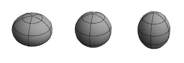
Figure 1: Spheroids for different ratios of polar radius ($r_{c}$) to equatorial radius ($r_{a}$). Here, the shapes have been plotted for different values $r_{c}/r_{a}=0.75$ (left), $1.0$ (centre) and $1.25$ (right). The figure in the centre is a sphere while the left one is an oblate and the right one is a prolate.

In spherical polar coordinates the equation of a spheroid is

$$r(\theta,\phi)=\frac{r_{a}}{\sqrt{1-\left(1-\frac{r_{a}^{2}}{r_{c}^{2}}\right)\cos^{2}\theta}},$$ (46)

with $r_{a}>0,\theta\in[0,\pi]$ and $\phi\in[0,2\pi]$. In can be easily concluded from (46) that an oblate (a prolate) is a surface of revolution obtained by rotating an ellipse about its minor (major) axis. The shapes of spheroids for different values of $r_{c}/r_{a}$ are depicted in Fig. (1). The `mean radius' $R_{0}$ for a spheroid is given by

$$R_{0}=\frac{r_{a}r_{c}}{\sqrt{r_{a}^{2}-r_{c}^{2}}}\sinh^{-1}\left(\frac{\sqrt{r_{a}^{2}-r_{c}^{2}}}{r_{c}}\right).$$ (47)

Since it is an axisymmetric object, it has an azimuthal symmetry. So, the expansion coefficients $C_{a}^{b}$s are non-zero only for $b=0$ and even values of $a$. The magnitude of them fall rapidly after a few terms in the expansion. Using these expansion coefficients we have calculated the first few energy levels for spheroidal boundaries in the range $0.75\leq r_{c}/r_{a}\leq 1.25$ and the comparison between the analytic perturbative values and their respective numerical values for DBC and NBC is shown in the Figs. (2) and (3) respectively. In these plots, analytical values are denoted by lines of different styles whereas their numerical counterparts are displayed by dots of different shapes. Throughout the deformation the volume of the spheroid remain same.

Figure 2: Comparison of the eigenvalues obtained numerically (denoted by points) and analytically (denoted by lines) for a spheroidal boundary satisfying DBC for the first 29 states.

\psfrag{C}[c]{ \small{$r_{c}/r_{a}$}}\psfrag{e}[c]{Energy \small{$(E)$}}\includegraphics[scale={1.5}]{DsphTbw.eps}

Figure 3: Comparison of the eigenvalues obtained numerically (denoted by points) and analytically (denoted by lines) for a spheroidal boundary satisfying NBC for the first 39 states.

\psfrag{C}[c]{ \small{$r_{c}/r_{a}$}}\psfrag{e}[c]{Eigenvalue \small{$(E)$}}\includegraphics[scale={1.5}]{NsphTbw.eps}

III.2 Superegg boundary

A superellipse [26], a compromise between a rectangle and an ellipse, is also known as Lamé curve [27] and is represented by the equation

$$\frac{|x|^{t}}{a^{t}}+\frac{|y|^{t}}{b^{t}}=1,$$ (48)

with $t,a$ and $b$ are positive numbers. A superellipsoid is a generalisation of superellipse into three dimensions where both horizontal sections and vertical cross-section through the center are superellipses with different exponent. The equation for a superellipsoid is given by

$$\left(\frac{|x|^{t}}{a^{t}}+\frac{|y|^{t}}{b^{t}}\right)^{n/t}+\frac{|z|^{n}}{c^{n}}=1,$$ (49)

with $t,n,a,b$ and $c$ are positive numbers. It is clear from (49) that for a fixed value of $z$, the horizontal cross-section is a superellipse with exponent $t$ and the vertical cross-section through center is also a superellipse with a different exponent $n$.
A superegg [28] is a special case of superellipsoid where $a=b$ and $t=2$. Thus, the equation of a superegg becomes

$$\left|\frac{\sqrt{x^{2}+y^{2}}}{a}\right|^{n}+\left|\frac{z}{c}\right|^{n}=1,$$ (50)

where $a$ is the horizontal radius at the equator and $2c$ is the height of the superegg with exponent $n$. It is to be noted that, a superegg with the exponent $n=2$ becomes a spheroid and along with that for the special case $a=c$, it reduces to a sphere of radius $a$.
The equation of a superegg in spherical polar coordinates is given by

$$r(\theta,\phi)=\frac{1}{\left(|\frac{\cos\theta}{c}|^{{}^{n}}+|\frac{\sin\theta}{a}|^{{}^{n}}\right)^{1/n}},$$ (51)

with $c,a$ and $n>0,\theta\in[0,\pi]$ and $\phi\in[0,2\pi]$. We have considered here the case $a=c=1$ only. It is clear to understand that a superegg is a surface of revolution by rotating a supercircle about either of its in-plane axes. The shapes of superegg for different values of the exponent $n$ are displayed in the Fig. (4). Since it is also an axisymmetric object, the expansion coefficients, $C^{b}_{a}$s are non-zero only for $b=0$. Moreover they survive for even values of $a$ and converge quickly. For the superegg shaped boundary we have calculated the first few energy levels using these expansion coefficients in the range $1.5\leq n\leq 3.0$ of the superegg exponent. The comparison between the analytic perturbative values and their numerical counterparts have been illustrated in Figs. (5) and (6) respectively for DBC and NBC. Here also, the analytical values are denoted by lines and the numerical ones are by dots.

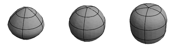
Figure 4: Shape of a superegg with $a=c=1$ for different values of the exponent $n$. Here, the figure in the centre is a sphere of unit radius ($n=2$) while the left and the right ones are supereggs for $n=1.5$ and $n=3$ respectively.

Figure 5: Comparison of the eigenvalues obtained numerically (denoted by points) and analytically (denoted by lines) for a superegg boundary satisfying DBC for the first 46 states.

\psfrag{n}[c]{Superegg exponent \small{$(n)$}}\psfrag{e}[c]{Energy \small{$(E)$}}\includegraphics[scale={1.5}]{DsegTbw.eps}

Figure 6: Comparison of the eigenvalues obtained numerically (denoted by points) and analytically (denoted by lines) for a superegg boundary satisfying NBC for the first 39 states.

\psfrag{n}[c]{Superegg exponent \small{$(n)$}}\psfrag{e}[c]{Eigenvalue \small{$(E)$}}\includegraphics[scale={1.5}]{NsegTbw.eps}

III.3 Superquadrics boundary

The equation of a general superquadric is given by

$$|x|^{a}+|y|^{b}+|z|^{c}=1$$ (52)

where $a$, $b$ and $c$ are real positive numbers. We restrict ourselves to the case $a=b=c=t$ only. For the exponent $t=1$, it becomes an octahedron, for $t=2$, it is a sphere and as $t\to\infty$ it converts to a cube.
The equation of a superquadric in spherical polar coordinates is given by

$$r(\theta,\phi)=\frac{1}{\left(|\sin\theta\cos\phi|^{{}^{t}}+|\sin\theta\sin\phi|^{{}^{t}}+|\cos\theta|^{{}^{t}}\right)^{1/t}},$$ (53)

with $t>0,\theta\in[0,\pi]$ and $\phi\in[0,2\pi]$. Our area of interest lies in the range $1\leq t\leq 20$. It is clear that the azimuthal symmetry is broken here unlike the above two cases. So, for this shape the expansion coefficients will now be non-zero for even values of $a\geq 4$ and $b\mod 4=0$. Since the general formalism is done for non-degenerate cases only and degenerate case requires axisymmetric perturbation, we restrict ourselves only to the non-degenerate cases. The shapes of the superquadric for different values of $t$ are shown in Fig. (7).

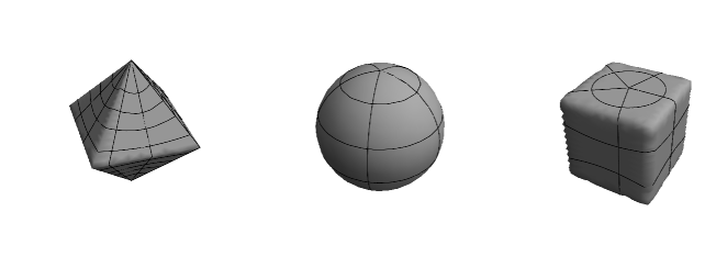
Figure 7: Shape of a superquadric for different values of the exponent $t$. Here, the figure in the centre is a sphere of unit radius ($t=2$) while the left one is an octahedron ($t=1$) and the right one is a superquadric for $t=20$.

For this boundary, we have calculated the eigenvalues for first three non-degenerate states (i.e. ground state, $9^{{\rm th}}$ excited state and $45^{{\rm th}}$ excited state) for DBC incorporating the second order eigenvalue corrections in the range $1\leq t\leq 20$ and compared them against the numerical results in Fig. (8).

Figure 8: Comparison of the eigenvalues obtained numerically (denoted by points) and analytically (denoted by lines) for a superquadric boundary satisfying DBC for the first three non-degenerate states ($l=0$).

\psfrag{n}[c]{ \small{$log\,(t)$}}\psfrag{e}[c]{Energy \small{$(E)$}}\includegraphics[scale={0.6}]{DsqdT.eps}

IV Conclusions

In this paper we have described an analytic formalism to determine the eigenspectrum of the Helmholtz equation in three dimensions for an arbitrary boundary subjected to either DBC or NBC. We have tested our perturbative results against the numerical values for two axisymmetric shapes $-$ spheroid, superegg and superquadric geometries. This is quite an achievement as numerical method was the only available method to solve the Helmholtz equation for such boundaries. In two dimensions, the Fourier decomposition of boundary perturbation was an obvious choice to take care of wide variety of boundary geometries. In three dimensional case for a general shape, to express the boundary asymmetries on the surface of a sphere, the natural basis is spherical harmonics. This specific form of boundary perturbation in terms of spherical harmonics will be effective to address a broad class of boundaries. In fact, the knowledge of spherical harmonic expansion coefficients and the `mean radius' for a given boundary is sufficient to get the eigenvalue and the wavefunction corrections. Also, to write down the corrections for eigenvalue and wavefunction exactly in closed form at each order of perturbation is indeed extraordinary. It is evident that the dominant contributions are coming from the first few orders. In the first order correction to the eigenvalue, one $C_{a}^{b}$ appears in the expressions, whereas in the second order correction we have a couple of $C_{a}^{b}$s appearing in the expression of eigenvalue. So, the convergence of spherical harmonic expansion coefficients ensures the convergence of the perturbative series for the eigenvalue correction. The only error in the series for eigenvalue correction is due to the truncation of the perturbative series up to second order. The perturbative scheme can handle both the degenerate and non-degenerate states in a same manner with ease for axisymmetric cases. Our method, even though perturbative in nature, works quite well for higher excited states and also for large deformation (which is against the very essence of the validity of a perturbative formalism). With the inclusion of higher order correction terms, which in principle can be obtained modulo their lengthy and cumbersome algebra, matching will definitely improve for the higher excited states. The $(2l+1)$ fold degeneracy of a degenerate state (with a given $l$ value) for the spherical boundary is lifted due to the deformation of a sphere. For a degenerate state, the eigenvalue corrections are equal for the same $|m|$ values out of all possible $m$ values. As a result of it, $l$ number of levels still remain degenerate and we get $(l+1)$ distinct energy levels. As an example we can say for $l=2$, we should have $5$ distinct energy levels but we get only three - one for $l=2,m=0$ and the other two levels are for $l=2,m=\pm 1$ and $l=2,m=\pm 2$ respectively. For DBC, in the case of spheroid and superegg boundaries we have compared numerical and analytical energy levels up to $29^{{\rm th}}$ and $46^{{\rm th}}$ state (including degeneracies) respectively. Similarly for NBC first $39$ states (including degeneracies) are compared. The matching of eigenvalues between analytic and numerical values are outstanding for superegg compared to spheroid for both the cases which is quite like their 2D analogues where the matching for supercircle was better than that for ellipses [8, 10]. For a larger deformation and for higher excited states in the case of spheroidal boundary the matching becomes less satisfactory. In these cases, the numerical methods may not be very accurate. It is evident from the plots that while the analytical method suggests exact degeneracy of some of the higher states throughout the entire range of deformation, the numerical counterparts split after certain range. So, the apparent disagreement is due to the limitation of numerical schemes rather than the failure of perturbative method. In case of superquadric geometries, the matching between the perturbative value and numerical value for the ground state is extraordinary. Maximum error occurs for octahedron which is $\sim 5\%$ and this is acceptable as octahedron can hardly be treated as a perturbation from sphere. On the other end, as $t\to\infty$, the superquadric converts to a cube. So, for high value of $t$, say $20$, the shape looks like a cube and for that shape we have compared analytic values against numerical ones and the discrepancy is $\sim 2\%$ and the eigenvalues tend towards the respective values for the cube which are $\frac{3}{4}\pi^{2},\,4\pi^{2}$ and $\frac{27}{4}\pi^{2}$.

In conclusion, we observe that the spherical harmonic expansion of the boundary perturbation will take care of wide variety of boundaries in three dimensions. To be able to write down the closed form solution at each order of perturbation is a unique feature of this method.

V Acknowledgments

SP would like to acknowledge the Council of Scientific and Industrial Research (CSIR), India for providing the financial support. The authors would like to thank S. Pratik Khastgir for useful discussions and a careful reading of the manuscript.

Appendix A Generalisation of Rayleigh's theorem in 3D

In our formalism, the energyspectrum of an arbitrary boundary has been approximated as a perturbation about a sphere of `average radius' and perturbative closed-form corrections to the equivalent spherical boundary at each order of perturbation have been obtained. Here, we will justify the above assumption for both DBC and NBC extending Rayleigh's proof for 2D [2] .

A.1 Particle in a 3D box and DBC

In the following, we will investigate how the wavefunction of a quantum particle confined in a spherical box is changed by a slight deviation from the exact spherical shape.
Independent of the shape of the boundary, $\psi$, the wavefunction of the particle satisfies the wave equation (in spherical polar co-ordinate system) everywhere inside the box

$$\frac{\partial^{2}\psi}{\partial r^{2}}+\frac{2}{r}\frac{\partial\psi}{\partial r}+\frac{1}{r^{2}}\left(\frac{\partial^{2}\psi}{\partial\theta^{2}}+\cot\theta\frac{\partial\psi}{\partial\theta}+\frac{1}{\sin^{2}\theta}\frac{\partial^{2}\psi}{\partial\phi^{2}}\right)+k^{2}\psi=0,$$ (54)

where $k^{2}$ is proportional to the energy of the particle to be determined subjected to the boundary condition $\psi=0$ on the boundary. Now, $\psi$ can always be expanded in the following series

$$\psi=\psi_{0}+\sum\limits_{l=1}^{\infty}\sum\limits_{m=-l}^{l}\psi_{l}\leavevmode\nobreak\ Y_{l}^{m}\,,$$ (55)

where $\psi_{0}$, $\psi_{1}$, $\cdots$, $\psi_{l}$ are functions of $r$ only. Plugging (55) in (54) we obtain that,

$$\sum\limits_{l=0}^{\infty}\sum\limits_{m=-l}^{l}\left\{\frac{d^{2}\psi_{l}}{dr^{2}}+\frac{2}{r}\frac{d\psi_{l}}{dr}+\left(k^{2}-\frac{l(l+1)}{r^{2}}\right)\psi_{l}\right\}Y_{l}^{m}=0,$$ (56)

which gives us $\psi_{l}\propto j_{l}(kr)$ as the other solution of (56) blows up at the origin. So, the general solution is given by

$$\psi=a_{0}\leavevmode\nobreak\ j_{0}(kr)+\sum\limits_{l=1}^{\infty}\sum\limits_{m=-l}^{l}a_{l}^{m}\leavevmode\nobreak\ j_{l}(kr)\leavevmode\nobreak\ Y_{l}^{m}.$$ (57)

The boundary condition dictates us that $\psi$ has to vanish on the boundary for all $\theta$ and $\phi$. Now, in the case of a nearly spherical well the radius vector is almost constant and can be approximated as $r=R_{0}+\delta r$, where $\delta r$ is a small quantity which can be function of both $\theta$ and $\phi$. So, the boundary condition $(\psi=0)$ now becomes

$$a_{0}\leavevmode\nobreak\ j_{0}(k(R_{0}+\delta r))+\sum\limits_{l=1}^{\infty}\sum\limits_{m=-l}^{l}a_{l}^{m}\leavevmode\nobreak\ j_{l}(k(R_{0}+\delta r))\leavevmode\nobreak\ Y_{l}^{m}=0.$$ (58)

Taylor expanding (58) about $r=R_{0}$ we get,

$$a_{0}\left\{j_{0}(kR_{0})+k\leavevmode\nobreak\ \delta r\leavevmode\nobreak\ j^{\prime}_{0}(kR_{0})\right\}+\sum\limits_{l=1}^{\infty}\sum\limits_{m=-l}^{l}a_{l}^{m}\left\{j_{l}(kR_{0})+k\leavevmode\nobreak\ \delta r\leavevmode\nobreak\ j^{\prime}_{l}(kR_{0})\right\}Y_{l}^{m}=0.$$ (59)

Let us first consider the nearly symmetrical normal modes and for which we can approximate

$$\psi=a_{0}\leavevmode\nobreak\ j_{0}(kr).$$

All the remaining coefficients will be small compared to $a_{0}$ as the boundary is deviated a little from the sphere. Taking the terms up to first order of smallness, we simplify (59) as

$$a_{0}\left\{j_{0}(kR_{0})+k\leavevmode\nobreak\ \delta r\leavevmode\nobreak\ j^{\prime}_{0}(kR_{0})\right\}+\sum\limits_{l=1}^{\infty}\sum\limits_{m=-l}^{l}a_{l}^{m}\leavevmode\nobreak\ j_{l}(kR_{0})\leavevmode\nobreak\ Y_{l}^{m}=0.$$ (60)

Now, integrating the above expression (60) with respect to $\theta$ and $\phi$ between the proper limits, we obtain the following for any arbitrary $a_{0}$ as

$$j_{0}(kR_{0})+\frac{k\leavevmode\nobreak\ j^{\prime}_{0}(kR_{0})}{4\pi}\int\limits_{\theta=0}^{\pi}\int\limits_{\phi=0}^{2\pi}\delta r\,\sin\theta\,\rm{d}\theta\,\rm{d}\phi=0,$$

or

$$j_{0}\left[k\left(R_{0}+\frac{1}{4\pi}\int\limits_{\theta=0}^{\pi}\int\limits_{\phi=0}^{2\pi}\delta r\,\sin\theta\,\rm{d}\theta\,\rm{d}\phi\right)\right]=j_{0}\left[k\left(R_{0}+\langle\delta r\rangle\right)\right]=0,$$ (61)

where

$$\langle\delta r\rangle=\frac{1}{4\pi}\int\limits_{\theta=0}^{\pi}\int\limits_{\phi=0}^{2\pi}\delta r\,\sin\theta\,\rm{d}\theta\,\rm{d}\phi,$$

is the average value of the change of radius from the exact spherical shape. (61) shows that the ground state energy of a particle in a slightly deformed spherical box is nearly equal to that of a spherical box with radius $R_{0}+\langle\delta r\rangle$ (= mean radius of the deformed box).

A.2 Standing waves in 3D enclosures and NBC

We now investigate the effect of slight deviation from the exact spherical shape on the normal modes of a spherical cavity.
Independent of the shape of the boundary, $\psi$ which is identified as a velocity potential, satisfies the wave equation (54) everywhere inside the sphere. Here $k$ is proportional to the frequency of the normal mode to be determined subjected to the boundary condition $\partial_{n}\psi=0$, i.e. the normal component of the velocity vanishing on the boundary. Like the earlier case, $\psi$ can be expanded in the series given by (55) and (57) gives the appropriate general solution. The boundary condition dictates us that $\partial_{n}\psi$ has to vanish on the boundary for all $\theta$ and $\phi$. Now, in the case of a nearly spherical cavity the radius vector is almost constant and can be approximated as $r=R_{0}+\delta r$, where $\delta r$ is a small quantity which can be function of both $\theta$ and $\phi$. So, the boundary condition ($\partial_{n}\psi=0$) now becomes

$$a_{0}\leavevmode\nobreak\ j^{\prime}_{0}(k(R_{0}+\delta r))+\sum\limits_{l=1}^{\infty}\sum\limits_{m=-l}^{l}a_{l}^{m}\leavevmode\nobreak\ j^{\prime}_{l}(k(R_{0}+\delta r))\leavevmode\nobreak\ Y_{l}^{m}-\frac{1}{r^{2}}\sum\limits_{l=1}^{\infty}\sum\limits_{m=-l}^{l}a_{l}^{m}\leavevmode\nobreak\ j_{l}(k(R_{0}+\delta r))\leavevmode\nobreak\ \hat{Y}_{l}^{m}\leavevmode\nobreak\ \hat{\delta r}$$

$$-\frac{1}{r^{2}\sin^{2}\theta}\sum\limits_{l=1}^{\infty}\sum\limits_{m=-l}^{l}a_{l}^{m}\leavevmode\nobreak\ j_{l}(k(R_{0}+\delta r))\leavevmode\nobreak\ \check{Y}_{l}^{m}\leavevmode\nobreak\ \check{\delta r}=0,$$ (62)

where the notations are explained in the text after (22). Taylor expanding (62) about $r=R_{0}$ we get,

$$a_{0}\left\{j^{\prime}_{0}(kR_{0})+k\leavevmode\nobreak\ \delta r\leavevmode\nobreak\ j^{\prime\prime}_{0}(kR_{0})\right\}+\sum\limits_{l=1}^{\infty}\sum\limits_{m=-l}^{l}\left\{a_{l}^{m}\left\{j^{\prime}_{l}(kR_{0})+k\leavevmode\nobreak\ \delta r\leavevmode\nobreak\ j^{\prime\prime}_{l}(kR_{0})\right\}Y_{l}^{m}-\frac{a_{l}^{m}}{r^{2}}\left\{j_{l}(kR_{0})\right.\right.$$

$$\left.\left.+k\leavevmode\nobreak\ \delta r\leavevmode\nobreak\ j^{\prime}_{l}(kR_{0})\right\}\leavevmode\nobreak\ \hat{Y}_{l}^{m}\leavevmode\nobreak\ \hat{\delta r}-\frac{a_{l}^{m}}{r^{2}\sin^{2}\theta}\left\{j_{l}(kR_{0})+k\leavevmode\nobreak\ \delta r\leavevmode\nobreak\ j^{\prime}_{l}(kR_{0})\right\}\leavevmode\nobreak\ \check{Y}_{l}^{m}\leavevmode\nobreak\ \check{\delta r}\right\}=0.$$ (63)

Let us first consider the nearly symmetrical normal modes and for which we can approximate

$$\psi=a_{0}\leavevmode\nobreak\ j_{0}(kr).$$

All the remaining coefficients will be small compared to $a_{0}$ as the boundary is deviated a little from the sphere. Taking the terms up to first order of smallness, we simplify (63) as

$$a_{0}\left\{j^{\prime}_{0}(kR_{0})+k\leavevmode\nobreak\ \delta r\leavevmode\nobreak\ j^{\prime\prime}_{0}(kR_{0})\right\}+\sum\limits_{l=1}^{\infty}\sum\limits_{m=-l}^{l}a_{l}^{m}\leavevmode\nobreak\ j^{\prime}_{l}(kR_{0})\leavevmode\nobreak\ Y_{l}^{m}=0.$$ (64)

Now, integrating the above expression (64) with respect to $\theta$ and $\phi$ between the proper limits, we obtain the following for any arbitrary $a_{0}$ as

$$j^{\prime}_{0}(kR_{0})+\frac{k\leavevmode\nobreak\ j^{\prime\prime}_{0}(kR_{0})}{4\pi}\int\limits_{\theta=0}^{\pi}\int\limits_{\phi=0}^{2\pi}\delta r\leavevmode\nobreak\ \sin\theta\,\rm{d}\theta\,\rm{d}\phi=0,$$

or

$$j^{\prime}_{0}\left[k\left(R_{0}+\frac{1}{4\pi}\int\limits_{\theta=0}^{\pi}\int\limits_{\phi=0}^{2\pi}\delta r\leavevmode\nobreak\ \sin\theta\rm{d}\theta\rm{d}\phi\right)\right]=j^{\prime}_{0}\left[k\left(R_{0}+\langle\delta r\rangle\right)\right]=0,$$

where again

$$\langle\delta r\rangle=\frac{1}{4\pi}\int\limits_{\theta=0}^{\pi}\int\limits_{\phi=0}^{2\pi}\delta r\leavevmode\nobreak\ \sin\theta\,\rm{d}\theta\,\rm{d}\phi,$$

is the average value of the change of radius from the exact spherical shape. The above result proves that the frequencies of the vibration of symmetrical normal modes are approximately the same as those of a spherical enclosure with the radius having the `mean value', $R_{0}+\langle\delta r\rangle$.

Appendix B Some useful formulae for Spherical harmonics and Clebsch-Gordan coefficients

We have used the following two identities (I, II) for the simplification of the product of spherical harmonics (the notations are explained in the text earlier). To best of our knowledge the identities V and VI are reported for the first time.

1. $$Y_{l_{1}}^{m_{1}}Y_{l_{2}}^{m_{2}}=\sum^{l_{1}+l_{2}}\limits_{l=\left\lceil\begin{subarray}{c}|l_{1}-l_{2}|\\ |m_{1}+m_{2}|\end{subarray}\right\rceil}\sqrt{\frac{(2l_{1}+1)(2l_{2}+1)}{4\pi(2l+1)}}\leavevmode\nobreak\ Y_{l}^{m_{1}+m_{2}}\langle l_{1}l_{2}00|l0\rangle\langle l_{1}l_{2}m_{1}m_{2}|l(m_{1}+m_{2})\rangle;$$

2. $$Y_{l_{1}}^{m_{1}}Y_{l_{2}}^{m_{2}}Y_{l_{3}}^{m_{3}}=\sum^{l_{1}+l_{2}}\limits_{k_{1}=\left\lceil\begin{subarray}{c}|l_{1}-l_{2}|\\ |m_{1}+m_{2}|\end{subarray}\right\rceil}\sum^{k_{1}+l_{3}}\limits_{k_{2}=\left\lceil\begin{subarray}{c}|k_{1}-l_{3}|\\ |m_{1}+m_{2}+m_{3}|\end{subarray}\right\rceil}\sqrt{\frac{(2l_{1}+1)(2l_{2}+1)(2l_{3}+1)}{16\pi^{2}\leavevmode\nobreak\ (2k_{2}+1)}}\leavevmode\nobreak\ Y_{k_{2}}^{m_{1}+m_{2}+m_{3}}$$

   $$\langle l_{1}l_{2}00|k_{1}0\rangle\langle l_{1}l_{2}m_{1}m_{2}|k_{1}(m_{1}+m_{2})\rangle\langle k_{1}l_{3}00|k_{2}0\rangle\langle k_{1}l_{3}(m_{1}+m_{2})m_{3}|k_{2}(m_{1}+m_{2}+m_{3})\rangle;$$

3. $$\hat{Y}^{b}_{a}\equiv\frac{\partial Y^{b}_{a}}{\partial\theta}=\frac{1}{2}\left\{\sqrt{(a-b)(a+b+1)}\leavevmode\nobreak\ Y^{b+1}_{a}-\sqrt{(a+b)(a-b+1)}\leavevmode\nobreak\ Y^{b-1}_{a}\right\};$$

4. $$\langle aa00|00\rangle\langle aab(-b)|00\rangle=(-1)^{b}\,(2a+1)^{-1};$$

5. 1. $$\sqrt{(l+m)(l-m+1)}\langle al1(m-1)|pm\rangle+\sqrt{(l-m)(l+m+1)}\langle al(-1)(m+1)|pm\rangle$$

      $$=-\left\{\frac{a(a+1)+(l-p)(l+p+1)}{\sqrt{a(a+1)}}\right\}\langle al0m|pm\rangle;$$

   2. $$\sqrt{(l+m)(l-m+1)}\langle al1(m-1)|lm\rangle+\sqrt{(l-m)(l+m+1)}\langle al(-1)(m+1)|lm\rangle$$

      $$=-\sqrt{a(a+1)}\langle al0m|lm\rangle;$$

6. $$\sqrt{b(b+1)}\langle ab0(-1)|k(-1)\rangle+\sqrt{a(a+1)}\langle ab(-1)0|k(-1)\rangle=\sqrt{k(k+1)}\langle ab00|k0\rangle.$$

References

- [1] I. Sobchenko, J. Pesicka, D. Baither, R. Reichelt, and E. Nembach. Superellipsoids: A unified analytical description of the geometry of nanoscale second-phase particles of any shape. Applied Physics Letters, 89(13):133107, 2006.
- [2] J. W. S. Rayleigh. The Theory of Sound. Dover Publications, New York, 1945. Vol 1, 2d ed.
- [3] P. M. Morse and H. Feshbach. Methods of Theoretical Physics, Part I. McGraw-Hill, New York, 1953.
- [4] J. W. S. Rayleigh. The Theory of Sound. Dover Publications, New York, 1945. Vol 2, 2d ed.
- [5] P. M Morse. Vibration and Sound. McGraw-Hill Kogakusha, Tokyo, 1948.
- [6] W. W. Read. Analytical solutions for a Helmholtz equation with Dirichlet boundary conditions and arbitrary boundaries. Math. Comput. Modelling, 24(2):23–34, 1996.
- [7] R. G. Parker and C. D. Mote Jr. Exact boundary condition perturbation for eigensolutions of the wave equation. Journal of Sound and Vibration, 211(3):389 – 407, 1998.
- [8] S. Chakraborty, J. K. Bhattacharjee, and S. P. Khastgir. An eigenvalue problem in two dimensions for an irregular boundary. Journal of Physics A: Mathematical and General, 42(19):195301–+, May 2009.
- [9] P. Amore. Spectroscopy of drums and quantum billiards: Perturbative and nonperturbative results. Journal of Mathematical Physics, 51(5):052105, May 2010.
- [10] S. Panda, S. Chakraborty, and S. P. Khastgir. Eigenvalue problem in two dimensions for an irregular boundary: Neumann condition. The European Physical Journal Plus, 126:1–20, 2011. 10.1140/epjp/i2011-11062-4.
- [11] S. Panda, T. G. Sarkar, and S. P. Khastgir. Metric deformation and boundary value problems in 2d. Progress of Theoretical Physics, 127(1):57–70, 2012.
- [12] B. A. Troesch and H. R. Troesch. Eigenfrequencies of an elliptic membrane. Mathematics of Computation, 27(124):pp. 755–765, 1973.
- [13] M. Robnik. Quantising a generic family of billiards with analytic boundaries. Journal of Physics A: Mathematical and General, 17(5):1049, 1984.
- [14] L. M. Cureton and J. R. Kuttler. Eigenvalues of the Laplacian on regular polygons and polygons resulting from their dissection. J. Sound Vibration, 220(1):83–98, 1999.
- [15] D. L. Kaufman, I. Kosztin, and K. Schulten. Expansion method for stationary states of quantum billiards. American Journal of Physics, 67(2):133–141, 1999.
- [16] E. Lijnen, L. F. Chibotaru, and A. Ceulemans. Radial rescaling approach for the eigenvalue problem of a particle in an arbitrarily shaped box. Physical Review E, 77(1):016702, Jan 2008.
- [17] P. Amore. Solving the Helmholtz equation for membranes of arbitrary shape: numerical results. Journal of Physics A: Mathematical and General, 41(26):265206, July 2008.
- [18] S. A. Moszkowski. Particle states in spheroidal nuclei. Phys. Rev., 99:803–809, Aug 1955.
- [19] T. Prosen. Quantization of a generic chaotic 3D billiard with smooth boundary. I. Energy level statistics. Physics Letters A, 233:323–331, February 1997.
- [20] T. Prosen. Quantization of generic chaotic 3D billiard with smooth boundary. II. Structure of high-lying eigenstates. Physics Letters A, 233:332–342, February 1997.
- [21] H. Primack and U. Smilansky. The quantum three-dimensional sinai billiard - a semiclassical anlaysis. Physics Reports, 327:1–107, March 2000.
- [22] T. Papenbrock. Numerical study of a three-dimensional generalized stadium billiard. Physical Review E, 61:4626–4628, April 2000.
- [23] I. M. Erhan and H. Taseli. A model for the computation of quantum billiards with arbitrary shapes. Journal of Computational and Applied Mathematics, 194:227–244, October 2006.
- [24] H. Alt, C. Dembowski, H.-D. Gräf, R. Hofferbert, H. Rehfeld, A. Richter, R. Schuhmann, and T. Weiland. Wave dynamical chaos in a superconducting three-dimensional sinai billiard. Phys. Rev. Lett., 79:1026–1029, Aug 1997.
- [25] J. U. Nöckel and A. D. Stone. Ray and wave chaos in asymmetric resonant optical cavities. Nature, 385(6611):45–47, 1997.
- [26] M. Gardner. Mathematical carnival : a new round-up of tantalizers and puzzles from Scientific American. Vintage Books, New York, 1977.
- [27] N. T. Gridgeman. Lamé ovals. The Mathematical Gazette, 54(387):pp. 31–37, 1970.
- [28] E. W. Weisstein. Superegg (mathworld a wolfram web resource). http://mathworld.wolfram.com/Superegg.html. Accessed: 18/10/2012.