Inelastic cross sections and continuum transitions illustrated by ⁸Be results

Abstract

We use the two-alpha cluster model to describe the properties of ⁸Be. The $E2$-transitions in a two-body continuum can be described as bremsstrahlung in an inelastic scattering process. We compute cross sections as functions of initial energy for the possible $E2$-transitions from initial angular momenta $(0^{+},2^{+},4^{+},6^{+},8^{+})$. The dependence on the exact shape of potentials is very small when the low-energy scattering phase-shifts are the same. We relate to practical observables where energies of the emerging alpha-particles are restricted in various ways. The unphysical infrared contribution is removed. We find pronounced peaking for photon energies matching resonance positions. Contributions from intra-band transitions are rather small although substantial (and even dominating) for initial energies between resonances. Structure information are derived but both ${\cal B}^{(E2)}$ values and electromagnetic transition rates are ambiguous in the continuum.

I Introduction

Nuclear structure information is often obtained from reaction experiments. Elastic scattering is the conceptually simplest process which probes the interaction between the colliding particles. The same particles in initial and final states, but different relative energies, is an inelastic process where the missing energy must be in emitted photons (provided that the particles themselves remain non-excited). Such cross section measurements then carry information about continuum properties of the combined system of the two particles, and corresponding cluster properties are perhaps here especially pronounced. Clearly, structure and dynamics are entangled, and extraction of useful structure information is then a challenge.

More and more experiments probing continuum properties are in the pipeline. Cluster structures are known to be of extreme importance in light nuclei and in particular for astrophysical processes in the continuum. A number of models employ spatially limited sets of basis states where the continuum has disappeared. They provide directly structure information but such discretization is not necessarily leading to correct observable results. The dynamics of a given reaction process has been removed by assumptions of independence of decay process and initial and final scattering states.

Two-body scattering processes are completely determined by the phase shifts, which in principle can be reproduced by different potentials. This is especially obvious for low energies where only rather few partial waves contribute. This means that the unique constraint from cross sections is on the asymptotic behavior of the potentials which however can have different number of bound states and still precisely identical phase shifts. This immediately implies that the scattering wave functions may differ at short distances by a corresponding number of nodes. On the other hand, structure information is related to matrix elements of an operator between initial and final states. As a consequence, structure information is contained in the short-distance wave-function properties, and therefore we could expect a substantial interaction dependence.

In this report we shall investigate these problems by use of the simplest two-body process of inelastic $\alpha-\alpha$ scattering. This provides information about the continuum properties of ⁸Be. We shall calculate cross sections defined by specified initial and final state energies. We shall investigate dependence on energies and on the chosen $\alpha-\alpha$ interaction. We shall extract as much structure information of ⁸Be as possible, and in particular focus on ${\cal B}^{(E2)}$-values. However, these quantities require initial and final states connected by the electric quadrupole operator, and the appropriate continuum states are not a priory well defined.

Previous works provided cross sections from energies around the positions of the $2^{+}$ and $4^{+}$ resonances in ⁸Be lan86b ; lan86c ; kro87 ; dat05 ; hyl10 ; kir11 ; rog12 . The theoretical results lan86b ; lan86c ; kro87 are converging although important discrepancies still remain. In these works the structure information is extracted as ${\cal B}^{(E2)}$-values by assuming a Breit-Wigner shape for population of the decaying initial $2^{+}$ and $4^{+}$ resonances in ⁸Be. No continuum background contribution is considered.

The purpose of this work is to provide cross sections and ${\cal B}^{(E2)}$-values with the highest numerical accuracy, test the dependence on how the inherent continuum state divergence is removed, and investigate the effect of a different short-distance behavior of the wave functions produced by the use of different potentials. More precisely, we shall provide cross sections for energies covering all positions of the resonances, $J^{\pi}=2^{+},4^{+},6^{+},8^{+}$, and limited to windows of final state energies around lower-lying resonances. The latter information is directly related to structure characteristics and furthermore also the quantities measured in practice in experiments. We shall compare to the scarce pieces of previous theoretical and experimental results.

In Section II we describe the theoretical background needed for the calculations. The results are collected in Section III, which contains three subsections describing, respectively, the ⁸Be spectrum and its dependence on the two-body potentials, the electric quadrupole cross sections for specific transitions, and the total cross sections for different final energy windows. The extraction of the ${\cal B}^{(E2)}$ transition strengths is described in Section IV. We finish in Section V with a short summary and the conclusions.

II Cross section expressions

The inelastic two-body scattering process is described in detail in Ref. ald56 as a bremsstrahlung cross section (see also Ref. tan85 ). In particular, the total cross section for $E\lambda$-radiation is given by Eq.(9) of Ref.tan85 . Assuming a two-body collision involving two identical particles with charge $Z$ and zero spin, the cross section becomes:

$$\frac{d\sigma}{dE_{\gamma}}\bigg{|}_{\ell\rightarrow\ell^{\prime}}=\frac{8\pi^{2}Z^{2}e^{2}}{2^{2\lambda-2}k^{2}}\frac{(\lambda+1)(2\lambda+1)}{\lambda[(2\lambda+1)!!]^{2}}(2\ell+1)^{2}(2\ell^{\prime}+1)\left(\frac{E_{\gamma}}{\hbar c}\right)^{2\lambda+1}\bigg{|}\langle\ell 0;\lambda 0|\ell^{\prime}0\rangle W(\lambda\ell^{\prime}\ell 0;\ell\ell^{\prime})\int_{0}^{\infty}u_{\ell}(E,r)r^{\lambda}u_{\ell^{\prime}}(E^{\prime},r)dr\bigg{|}^{2}\;,$$ (1)

where $E$ and $E^{\prime}$ are the initial and final energies in the two-body center of mass frame, $E_{\gamma}=E-E^{\prime}$ is the energy of the emitted photon, $\ell$ and $\ell^{\prime}$ are the relative angular momenta between the two particles in the initial and final state, $k^{2}=2\mu E/\hbar^{2}$ ($\mu$ is the reduced mass of the two-body system), and $W$ represents a standard Racah coefficient.

The radial two-body wave functions $u_{\ell}$ and $u_{\ell^{\prime}}$ are solutions of the radial two-body Schrödinger equation with potential $V(r)$, and they obey the large-distance boundary condition

$$u_{\ell}(E,r)\stackrel{{\scriptstyle r\rightarrow\infty}}{{\longrightarrow}}\sqrt{\frac{2\mu}{\pi\hbar^{2}k}}\left[\cos\delta_{\ell}F_{\ell}(kr)+\sin\delta_{\ell}G_{\ell}(kr)\right],$$ (2)

where $F_{\ell}$ and $G_{\ell}$ are the regular and irregular Coulomb functions, $\delta_{\ell}$ is the nuclear phase shift, and the normalization constant is determined by the orthogonality condition:

$$\int_{0}^{\infty}u_{\ell}(E,r)u_{\ell}(E^{\prime},r)dr=\delta(E-E^{\prime}).$$ (3)

The total bremsstrahlung cross section is finally obtained after integration over the energy of the emitted photon:

$$\sigma(E)=\int\left.\frac{d\sigma}{dE_{\gamma}}\right|_{\ell\rightarrow\ell^{\prime}}(E)\;dE_{\gamma}\;,$$ (4)

where $E^{\prime}=E-E_{\gamma}$. In addition to the integration, a summation over all angular momenta, $\ell$ and $\ell^{\prime}$, as well as all multipolarities, $\lambda$, has to be included in Eq.(4). We shall avoid cluttering the notation by adding more indices. In any case we also want to keep track of the individual contributions.

The measurement is simply to control relative energy of two colliding particles, and identify the same outgoing particles and measure their energies. The computed cross sections should then be obtained in close analogy to the experimental setup, where only a finite range of final relative energies is measured. This means that the integral in Eq.(4) should be performed only over this precise energy range. We shall often refer to this range as the final energy window.

Once a two-body potential has been chosen, the procedure is clear from Eqs.(1) and (4), that is, find the wave functions and perform the integrals. However, some care must be exercised in the calculation of the matrix elements because the continuum wave functions, $u_{\ell}(r)$, cannot be normalized in coordinate space. The bare matrix elements diverge until a regularization procedure is employed. We shall follow the Zel’dovich prescription zel60 , which introduces the regularization factor $e^{-\eta^{2}r^{2}}$ in the radial integrand, such that the correct result is obtained in the limit of zero value for the Zel’dovich parameter $\eta$. Fortunately, this removes the unwanted large-distance contributions and the remaining physics results are uniquely defined, since they are stable for sufficiently small values of $\eta$. Obviously, the smaller the parameter $\eta$ the slower the fall off of the radial integrand, and therefore the larger the upper limit required in the radial integral in Eq.(1).

In order to compute inelastic cross sections the only remaining decision is to choose precisely which observable should be computed, that is which energy interval has to be employed in the integration (4). Except for practical experimental difficulties it is possible to choose any energy interval allowing emission of one photon. The advantage is that no additional information is required, as for example definition of a resonance or knowledge of the decay mechanism through an intermediate structure. This information is implicitly contained in the continuum wave functions. Note that when using Eq.(2) the energies $E$ and $E^{\prime}$ (and therefore also $E_{\gamma}$) are treated as continuum variables (the continuum is not discretized). The integral (4) can be easily performed within any arbitrary energy limits by choosing an also arbitrary small grid for the photon energy.

Direct comparison of precisely the same observables is then possible and desirable. However, an important question is whether the structure information can be disentangled from the measured cross sections. This is a standard procedure for bound states, and the obvious continuation is to apply the procedure to resonances. One option is to focus on final energy windows around peaks in the cross sections corresponding to (otherwise known) resonances. Interpretation in terms of multipole transitions may then be possible but may be also ambiguous if the results depend too much on the chosen energy windows. It is crucial to know if the structure information can in principle be extracted. In fact, most theoretical results are obtained without even realizing this problem because the continuum already is discretized and resonances therefore model dependently defined.

Finally, it is also important to know the dependence of these observables on the two-body potential. After all, different potentials providing identical phase shifts could produce wave functions with a different short-distance behavior, which therefore could also produce different radial integrals in Eq.(1) and different cross sections.

In the following section all these issues are investigated for the $\alpha-\alpha$ scattering process.

III Computed cross sections

The $\alpha-\alpha$ reaction is specified by initial and final state energies, as well as by the energy window for measured final energies. The angular momentum is at best only indirectly controlled in the experiment. However, knowledge of the two-body resonance properties allow substantiated expectation of dominating individual angular momenta at certain energy ranges. In particular, the cross section is expected to have peaks for incident energies in the vicinity of the ⁸Be resonances. For the two-body $\alpha$-structure of ⁸Be only even relative angular momenta and positive parity are allowed. This means that the lowest multipolarity of an electromagnetic transition must have $E2$ character. Therefore, the cross section is given by Eq.(1) for $Z=2$, $\lambda=2$, and where only even values of $\ell$ and $\ell^{\prime}$ are possible. Transitions with higher multipolarity, where $\lambda=4$ is the next allowed, are clearly smaller by several orders of magnitude ald56 ; bla79 .

III.1 Two-body potentials and ⁸Be spectrum

Table 1: Resonance energies, $E_{r}$, and widths, $\Gamma$, in MeV of the five lowest computed resonances in ⁸Be with angular momentum and parity $J^{\pi}$. Rows two and three give, when available, the corresponding experimental values taken from Ref.til04 . The following four rows are the computed values with the Buck and Ali-Bodmer-d potentials buc77 ; ali66 .

$J^{\pi}$	$0^{+}$	$2^{+}$	$4^{+}$	$6^{+}$	$8^{+}$
$E_{r}$ (Exp.)	0.0918	$2.94\pm 0.01$	$11.35\pm 0.15$	—	—
$\Gamma$ (Exp.)	$(5.57\pm 0.25)\times 10^{-6}$	$1.51\pm 0.02$	$\sim 3.5$	—	—
$E_{r}$ (Buck)	0.091	2.88	11.78	33.55	51.56
$\Gamma$ (Buck)	$3.6\times 10^{-5}$	1.24	3.57	37.38	92.38
$E_{r}$ (Ali-Bodmer-d)	0.092	2.90	11.70	34.38	53.65
$\Gamma$ (Ali-Bodmer-d)	$3.1\times 10^{-6}$	1.27	3.07	37.19	93.74

Two different potentials will be used for the $\alpha-\alpha$ interaction: The Buck potential buc77 and the d version of the Ali-Bodmer potential ali66 . Both of them are simple gaussian potentials that fit equally well the low-energy ($E<15$ MeV) $\alpha-\alpha$ phase shifts, not only for $\ell=0$, $\ell=2$, and $\ell=4$ lan86b , but also for $\ell=6$ and $\ell=8$. One of the differences between both potentials is that while the Buck potential is partial-wave independent, the Ali-Bodmer potential has been adjusted separately for each individual partial wave. The second and most important difference is in the treatment of the Pauli principle. The Buck potential contains two $s$-wave and one $p$-wave Pauli-forbidden bound states sai69 , which in the case of the Ali-Bodmer potential are automatically excluded by use of a repulsive potential, also with gaussian shape. A third alternative is to use the phase-equivalent version of the Buck potential, which is constructed in such a way that the Pauli-forbidden states are removed from the spectrum but keeping the phase shifts exactly the same. Then also the two-body resonances remain at exactly the same positions as for the original potential gar99 .

In table 1 we give the energies ($E_{r}$) and widths ($\Gamma$) of the lowest five resonances found in ⁸Be. They have been obtained by use of the complex scaling method, which permits to extract resonances as poles of the $S$-matrix and with the complex-scaled wave functions behaving asymptotically as bound states ho83 . The values in the second and third rows correspond to the experimentally known resonances til04 . As seen in the table, the two potentials used in this work give rise to very similar spectra, not only for the energies themselves, but also for the corresponding widths. The computed widths for the experimentally unknown $6^{+}$ and $8^{+}$ resonances are rather big, which means that even if they appear as poles of the $S$-matrix they are pretty much diluted in the two-body continuum. They can hardly be characterized as resonances related to observables.

III.2 Electric quadrupole cross sections

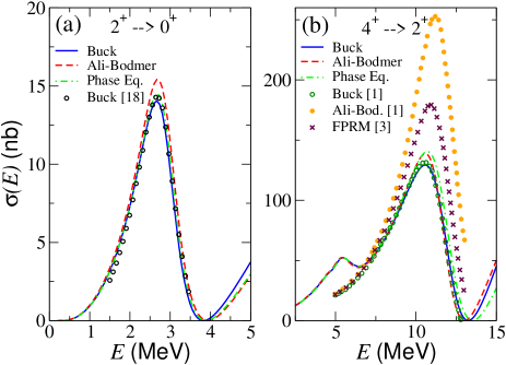
Figure 1: (Color online) Integrated cross section (Eq.(4)) for the $2^{+}\rightarrow 0^{+}$ (a) and $4^{+}\rightarrow 2^{+}$ (b) transitions as function of initial energy. Results using the Buck potential (solid curves), the Ali-Bodmer-d potential (dashed curves), and the phase equivalent version of the Buck potential (dot-dashed curves) are shown. In (a), the open circles are the result given in lan86 . In (b), the open and closed circles are the results given in lan86b obtained with the Buck and Ali-Bodmer potentials, respectively, and the crosses are the cross section calculated in kro87 using the Buck potential and the Finite Pauli Repulsion Model.

Let us start by investigating the dependence of the cross section on the $\alpha-\alpha$ potential. As already mentioned, for $\alpha-\alpha$ collisions the $E2$ contribution dominates. In Fig.1 we show the computed electric quadrupole cross sections for the $2^{+}\rightarrow 0^{+}$ (left part) and $4^{+}\rightarrow 2^{+}$ (right part) transitions. They have been obtained according to Eqs.(1) and (4). For the $2^{+}\rightarrow 0^{+}$ case, due to the extremely small width of the $0^{+}$ resonance (just a few ev, see table 1), the final energy window for the integration in Eq.(4) has been taken very small, of only 0.5 keV, which is far smaller than the best experimental resolution of about $10$ keV. For the $4^{+}\rightarrow 2^{+}$ reaction we have chosen the same final energy interval as in lan86b ; lan86c ; kro87 , namely, $2\mbox{ MeV}<E^{\prime}<4\mbox{ MeV}$, which corresponds roughly to the $2^{+}$ resonance energy $\pm 1$ MeV.

In the figure the solid, dashed, and dot-dashed curves correspond to the cross sections obtained with the Buck potential buc77 , the Ali-Bodmer-d potential ali66 , and the phase equivalent Buck potential gar99 , respectively. As we can see, for both transitions the computed cross sections are quite similar to each other for the different potentials. This similarity is also found in spite of the fact that the nodes in the scattering wave functions are different although the phase shifts are the same. The surprise is that the transition probability is determined by a matrix element between these wave functions. It could then easily have depended on the nodes, but the contribution is apparently determined by the identical structure at large distances.

Improvement in conceptual or numerical accuracy is exhibited by comparison to deviating previous calculations. In particular, in Fig. 1b the closed circles are the results reported in lan86b , where the Ali-Bodmer potential was used, and the crosses correspond to the cross section given in kro87 , where the Buck potential and the Finite Pauli Repulsion Model was used. However, the calculations in lan86 (open circles in Fig.1a) and lan86b (open circles in Fig.1b) corresponding to the $2^{+}\rightarrow 0^{+}$ and $4^{+}\rightarrow 2^{+}$ transitions, respectively, and performed both with the Buck potential, agree very nicely with our calculations with the same potential.

The cross sections in Fig.1 have been obtained with a Zel’dovich parameter of $\eta=0.02$ fm^-1. For this value the computed cross sections are already stable when going to the limit $\eta\rightarrow 0$. In principle, smaller values could have been used, but the smaller $\eta$ the larger the distance up to which the integral in Eq.(1) has to be performed. The increase of the integration distance makes the numerical calculation of the integral more and more complicated due to the strongly oscillating behavior of the integrand. In any case, $\eta$ values up to twenty times smaller than the one used in Fig.1 produce cross sections that are indistinguishable from the ones shown in the figure.

In all the cases the general behavior of the cross sections in Fig.1 is qualitatively very similar. The energy dependence exhibits a pronounced peak at about the $2^{+}$ resonance energy in Fig.1a, and about the $4^{+}$ resonance energy in Fig.1b (see table 1). After decrease through a minimum the cross section increases at higher energies due to the advantage of an increasing photon energy, see Eq.(1), and a fair match between some of the continuum states.

In Fig.1b a remarkable feature in the cross section appears at small energies. The decrease of the integrated cross section with decreasing energy continues all the way to the threshold. However, the decrease is not smooth, and a small bump is observed. It is important to note that the bump appears precisely in the region where the initial energy $E$ approaches the upper limit of the energy window of final energies $E^{\prime}$ ($\sim$4.0 MeV). This means the bump appears in the region where the photon energy ($E_{\gamma}=E-E^{\prime}$) takes small values. For the $2^{+}\rightarrow 0^{+}$ reaction (Fig.1a) this bump is actually not seen due to the very small energy and width of the $0^{+}$ resonance and the very small size of the corresponding energy window.

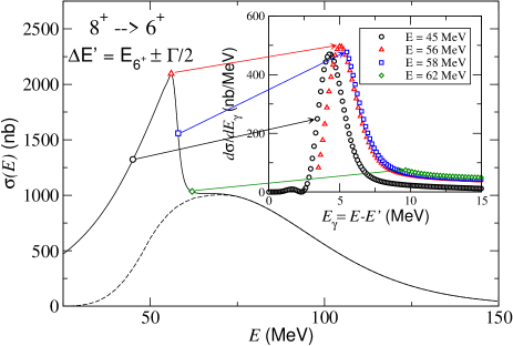
Figure 2: (Color online) Outer part: Integrated cross section for the $8^{+}\rightarrow 6^{+}$ transition in ⁸Be with a final energy window of $E_{6^{+}}\pm\Gamma/2$. The solid and dashed curves are the calculation including and excluding the soft-photon contributions, respectively. Inner part: Differential cross section (integrand of Eq.(4)) as a function of the photon energy $E_{\gamma}$ for the initial energy values $E=45$ MeV (circles), $E=56$ MeV (triangles), $E=58$ MeV (squares), and $E=62$ MeV (diamonds).

To exhibit the origin of this bump, we shall consider the theoretical transition of $8^{+}\rightarrow 6^{+}$. According to table 1, at least theoretically, the $8^{+}$ and $6^{+}$ resonances have a fairly large width, with a substantial overlap between both resonances. In the outer part of Fig.2 the solid line shows the $8^{+}\rightarrow 6^{+}$ cross section computed following Eqs.(1) and (4) with the Buck potential. Only final energies within the window $E_{6^{+}}\pm\Gamma/2$ have been considered ($E_{6^{+}}$ and $\Gamma$ are the energy and width of the $6^{+}$ resonance). This means that the upper limit of the window is about 53 MeV. As we can see in the figure, for energies below this value the cross section shows a huge bump that does not match at all with the smooth behavior of the cross section obtained for higher energies. This huge bump has the same origin as the small bump observed in Fig.1b.

To understand the origin of this bump it is very clarifying to look into the differential cross sections for some specific values of the initial energy $E$ (integrand of Eq.(4) for given values of $E$). This is shown in the inner part of Fig.2 as a function of the photon energy for initial energy values $E=45$ MeV (circles), $E=56$ MeV (triangles), $E=58$ MeV (squares), and $E=62$ MeV (diamonds). Integration of the differential cross section as indicated in (4) gives rise to the total cross section indicated in the outer part of the figure by the same symbols.

As we can see, for $E=62$ MeV, where the total cross section is still out of the bump, the differential cross section shown in the inset is rather flat (diamonds), without any particular structure. The minimum value of $E_{\gamma}$ is of about 9 MeV, which is the difference between $E$ (62 MeV) and the upper part of the energy window for $E^{\prime}$ (53 MeV). However, for $E=58$ MeV a sharp increase appears in the differential cross section (squares). This increase becomes a well defined and almost complete peak for $E=56$ MeV (triangles), which produces the maximum of the bump in the cross section. For $E=45$ MeV (circles) the peak in the differential cross section is now complete, but it is a bit smaller than for $E=56$ MeV, which gives rise to an also smaller total cross section.

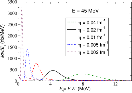
Figure 3: (Color online) Differential cross section (integrand of Eq.(4)) as a function of the photon energy $E_{\gamma}$ for the $8^{+}\rightarrow 6^{+}$ transition in ⁸Be. The initial energy is $E=45$ MeV and a final energy window of $E_{6^{+}}\pm\Gamma/2$ has been used. The different curves correspond to different values of the Zel’dovich parameter $\eta$ used to regularize the continuum wave functions.

The nature of this peak in the differential cross section is shown in Fig.3. In fact, although the total cross section does not depend on the Zel’dovich parameter (provided that the value is small enough), the differential cross section does show a dependence on the Zel’dovich parameter. In Fig.3 we show the same differential cross section as in the inset of Fig.2 for an initial energy $E=45$ MeV and for different values of $\eta$. In all the cases the integrated cross section is about the same, but as $\eta$ decreases the peak of the differential cross section moves towards zero and becomes sharper. In fact, in the limit of very small $\eta$ values the peak would be extremely sharp and located basically at $E_{\gamma}=0$.

This behavior of the differential cross section is actually showing the known $1/E_{\gamma}$ dependence of the bremsstrahlung cross section at small photon energies gre01 . This is the so called infrared catastrophe. This divergence is behind the appearance of the bumps in the cross sections under discussion. However, as explained in gre01 , this divergence is not physical. A transition with $E_{\gamma}=0$ is nothing but an elastic process. A relativistic treatment of the elastic reaction up to the same order will produce a similar $1/E_{\gamma}$ divergence in the cross section but with opposite sign that precisely cancels the one obtained in the calculation of the bremsstrahlung cross section.

A simple way of eliminating the unphysical contribution of the soft photons is to exclude from the integral in Eq.(4) the sharp peak in the differential cross section shown in Fig.3. When this is done, the resulting cross section for the $8^{+}\rightarrow 6^{+}$ transition is shown by the dashed line in the outer part of Fig.2. As we can see, exclusion of the soft photon contribution eliminates the bump in the cross section.

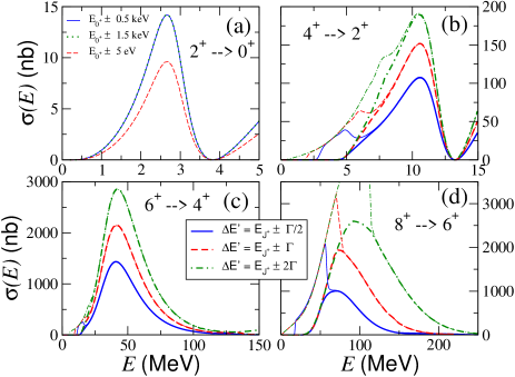
Figure 4: (Color online) Integrated cross sections (Eq.(4)) as a function of the initial energy, $E$, for the $2^{+}\rightarrow 0^{+}$, $4^{+}\rightarrow 2^{+}$, $6^{+}\rightarrow 4^{+}$, and $8^{+}\rightarrow 6^{+}$ transitions (panels (a), (b), (c), and (d), respectively). In panel (a) the solid, dotted, and dashed curves correspond to final energy windows $E_{0^{+}}\pm 0.5$ keV, $E_{0^{+}}\pm 1.5$ keV, and $E_{0^{+}}\pm 5$ eV, respectively, where $E_{0^{+}}$ is the energy of the $0^{+}$ resonance in ⁸Be. In panels (b), (c), and (d) the solid, dashed, and dot-dashed curves correspond to final energy windows $E_{J^{\pi}}\pm\Gamma/2$, $E_{J^{\pi}}\pm\Gamma$, and $E_{J^{\pi}}\pm 2\Gamma$, respectively, where $E_{J^{\pi}}$ and $\Gamma$ are the energy and width of the resonance in the final state with spin and parity $J^{\pi}$. The thick and thin curves are the calculations with and without exclusion of the soft-photon contributions, respectively.

Finally, in Fig.4 we show how the cross sections for the different transitions depend on the energy window chosen for the final state. Due to the close similarity observed in Fig.1 for the different potentials it suffices to show results for only one of them, e.g. the Buck potential.

For the $2^{+}\rightarrow 0^{+}$ transition, due to the very small width of the $0^{+}$ resonance, an energy window of 0.5 keV around the resonance energy already maximizes the cross section. In fact, when a window three times wider ($E_{0^{+}}\pm 1.5$ keV) is used, both cross sections are completely indistinguishable (solid and dotted curves in Fig.4a). In order to observe some variation an extremely narrow window should be considered. As an example, the dashed curve in the figure shows the cross section obtained with an energy window of only $E_{0^{+}}\pm 5$ eV. In this case the maximum of the cross section decreases from about 14 nb to a bit less than 10 nb.

In Figs. 4b, 4c, and 4d the energy windows $E_{J^{\pi}}\pm\Gamma/2$ (thick-solid curves), $E_{J^{\pi}}\pm\Gamma$ (thick-dashed curves), and $E_{J^{\pi}}\pm 2\Gamma$ (thick-dot-dashed curves) have been used, where $E_{J^{\pi}}$ and $\Gamma$ are the energy and width, respectively, of the resonance in the final state with spin and parity $J^{\pi}$. The corresponding thin curves are the cross sections obtained when the soft-photon contribution is included. This results in the bump observed at small energies. As explained, the size of the bump is directly related to the overlap between the final energy window and the initial energy $E$. Even for the case of the largest energy window, the effect of the soft photons is limited to $E$-values below $\sim$6 MeV for the $4^{+}\rightarrow 2^{+}$ transition and below $\sim$18 MeV for the $6^{+}\rightarrow 4^{+}$ transition. Only for the $8^{+}\rightarrow 6^{+}$ transition, due to the large widths of the resonances involved, this effect is clearly visible.

We notice in Figs. 4b, 4c, and 4d that the increase of the size of the final energy window produces a significant increase of the cross sections. This may be attributed to the relatively broad final state resonances. The variation can reach up to a factor of 2 when changing from the smallest to the largest window. In comparison to measured values, this window dependence is therefore very important. It is tempting to discuss this window dependence as arising by a division into resonance-to-resonance decay and non-resonant continuum background contributions to the decay. Then, increase of the window width to be larger than $\Gamma$ (full width at half maximum) should entirely add only non-resonant contributions. Such a distinction can at this level never be sharp and well defined, although suggestive and probably even useful.

We emphasize that the window dependence so far has been only shown for initial and final state energies around resonance positions and for the corresponding set of angular momenta. In any case, these contributions are expected to be the dominating ones, as shown in the next subsection.

III.3 Total cross sections

The total cross section corresponding to the $E2$-transition for a given final energy window should contain not only the contributions shown in Fig.4, which correspond to some specific transitions with given initial and final angular momenta, but they should also contain the contributions from all the other possible $E2$ transitions to that precise final energy window. In fact, the observables are first of all the cross sections restricted to be functions of the chosen initial and final state energies, and the contributions from different types of transitions can not be directly distinguished. In particular, keeping aside the $8^{+}$ states, the $2^{+}\rightarrow 0^{+}$, $0^{+}\rightarrow 2^{+}$, $2^{+}\rightarrow 2^{+}$, $4^{+}\rightarrow 2^{+}$, $2^{+}\rightarrow 4^{+}$, $4^{+}\rightarrow 4^{+}$, $4^{+}\rightarrow 6^{+}$, $6^{+}\rightarrow 4^{+}$, and $6^{+}\rightarrow 6^{+}$ transitions could contribute to the total $E2$ cross section for a given final energy window.

To get a feeling on how these contributions can modify the cross sections shown in Fig.4, let us focus first on the transitions between states with equal angular momentum and with final energy windows around the resonance corresponding to that angular momentum. In other words, let us see how the $2^{+}\rightarrow 2^{+}$ transition contributes to the cross section in Fig.4b, where the final energy window is chosen around the $2^{+}$ resonance energy, and the same for the contribution of the $4^{+}\rightarrow 4^{+}$ and $6^{+}\rightarrow 6^{+}$ transitions to the cross sections in Figs.4c and 4d, respectively.

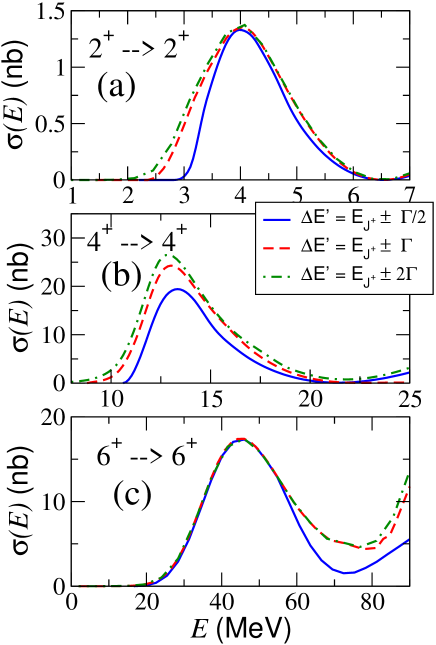
Figure 5: (Color online) The same as in Fig.4 for the transitions $2^{+}\rightarrow 2^{+}$, $4^{+}\rightarrow 4^{+}$, and $6^{+}\rightarrow 6^{+}$ (panels (a), (b), and (c), respectively). In all the calculations the soft-photon part has been excluded.

As in Fig.4, the contribution from the $2^{+}\rightarrow 2^{+}$, $4^{+}\rightarrow 4^{+}$, and $6^{+}\rightarrow 6^{+}$ transitions are expected to show a peak at an energy around one of the resonances in the initial state, which in this case obviously coincides with the resonance in the final state. These transitions can then be understood as intrastate transitions for initial energies within the energy window around the resonances. It is then clear that in this case the removal of the soft-photon contribution becomes crucial. The corresponding cross sections for the $2^{+}\rightarrow 2^{+}$, $4^{+}\rightarrow 4^{+}$, and $6^{+}\rightarrow 6^{+}$ transitions are shown in Fig.5. The meaning of the different curves and the sizes of the final energy windows are the same as in Fig.4 for each of the final $J^{+}$ states.

The curves in Fig.5 have been computed for each of the transitions by removing the contribution from the photon energies corresponding to the unphysical peak in the differential cross section analogous to the one shown in Fig.3. However, in this case, the bulk of the cross section is affected by the soft-photon contribution. Therefore, the computed cross section is very sensitive to the cutoff imposed to the photon energy. In fact, in general, the position of the peak to be removed in the differential cross section depends on the initial energy, and the photon-energy cutoff should then depend on this energy. The curves in Fig.5 are then estimates rather than accurate calculations. In any case, when comparing to the curves in Fig.4 with the same $J^{+}$ final state we observe that the contributions plotted in Fig.5 are rather small, and they could produce an increase in the vicinity of the maximum of the cross sections shown in Fig.4 of about 2 or 3%.

Another interesting contribution to be analyzed in more detail is the one coming from transitions where the initial angular momentum is lower than the final one. They are the transitions $0^{+}\rightarrow 2^{+}$, $2^{+}\rightarrow 4^{+}$, and $4^{+}\rightarrow 6^{+}$. They are characterized by the fact that the resonance associated to the initial angular momentum is lower than the one associated to the final angular momentum. When the final energy is limited to values within a window around the resonance, all the initial states will then be far from their corresponding resonance, and they would be essentially pure continuum states. As a consequence, the peak analogous to the one observed in Figs.4b, 4c, and 4d, located at an energy close to the one of the initial resonance, would not be there, and the contribution to the cross section is therefore expected to be not very relevant, and at most enhance the tail of the cross section.

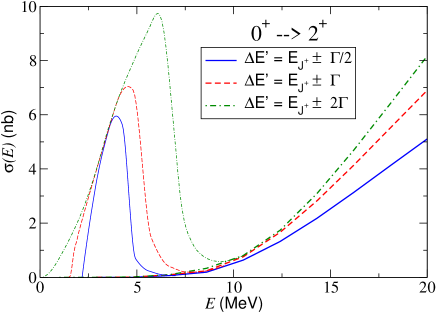
Figure 6: (Color online) The same as in Fig.4 for the $0^{+}\rightarrow 2^{+}$ transition.

As an illustration we show in Fig.6 the cross sections corresponding to the $0^{+}\rightarrow 2^{+}$ reaction for the three usual final energy windows. The thick curves correspond to calculations where the soft-photon contribution has been removed. The computed cross sections are small in the energy region corresponding to the peak in Fig.4b, and their main contribution appears at higher energies. As in Fig.2, the soft photons produce a sizable bump (thin curves) when the initial energies are within the energy window of the final state. Obviously the wider the final energy window the wider the energy range affected by the low-energy photons, and therefore the wider the bump. How much of the bump disappears after removal of the soft photons depends strongly on the cutoff imposed to the photon energy. A cutoff estimated from the width of the peak in the differential cross section (Fig.3) makes most of the bump disappear. In any case, even if the cross sections shown in Fig.6 are a bit shaky in the energy region corresponding to the bump, its weight is rather modest compared to the cross sections shown in Fig.4, at least for energies around the maximum, and it amounts to no more than a few percent of the total.

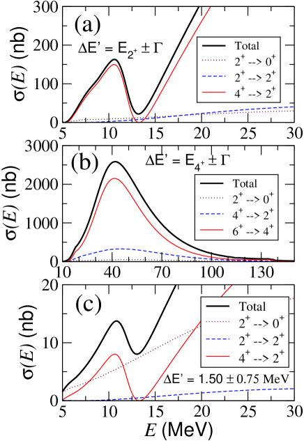
Figure 7: (Color online) Total $E2$ cross sections for final energy windows (a) $E_{2^{+}}\pm\Gamma$, (b) $E_{4^{+}}\pm\Gamma$ , and (c) $1.75\pm 0.75$ MeV. The total cross sections are given by the thick solid curves. Although all the possible transitions are included in the total, only the three of them giving the largest contributions are shown on each of the three panels.

Finally, in Fig.7 we show the total cross section for three different final energy windows. Together with the total, the three most relevant contributions among all the possible contributing transitions are also shown. In the upper and middle panels (Figs.7a and 7b) the windows have been chosen around the $2^{+}$ and the $4^{+}$ resonance energies ($\pm\Gamma$), respectively. In the lower part, Fig.7c, the final energy window has been taken in such a way it does not overlap with any of the known resonances in ⁸Be. In particular, we have chosen the energy window $1.5\pm 0.75$ MeV.

Fig.7a shows the expected peak from the leading resonance-to-resonance transition. The corresponding contribution was shown by the thick-dashed curve in Fig.4b, and it is now given by the thin-solid curve. This $4^{+}\rightarrow 2^{+}$ contribution dominates both at the resonance and beyond. The increase with energy is dramatic from zero just above the $4^{+}$ resonance energy to values much larger than at the resonance. This increase of the non-resonant contribution is much less than corresponding to the fifth power of the photon energy, which therefore reveals that the matrix elements are decreasing.

Only a few of the other possible non-resonant transitions produce a visible contribution to the cross section. These are the ones shown in the figure by the thin-dotted, thin-dashed, and thin-dot-dashed curves, which correspond, respectively, to the $2^{+}\rightarrow 0^{+}$, $2^{+}\rightarrow 2^{+}$, and $0^{+}\rightarrow 2^{+}$ transitions. They represent the smooth non-resonant background contributions which away from resonances (both final and initial energies) could be dominating. In any case, although visible, their weight is not very significant, and the total cross section (thick solid curve) follows the trend dictated by the resonance-to-resonance transition. At the resonance peak they increase the maximum of the cross section from about 150 nb to about 165 nb.

The cross section shown in Fig.7b shows a similar structure to the one in the upper panel. Now the resonance-to-resonance contribution correspond to the $6^{+}\rightarrow 4^{+}$ (thick-dashed curve in Fig.4c), and it is now given by the thin-solid curve. Among the remaining transitions only the $4^{+}\rightarrow 2^{+}$ gives a sizable contribution (dashed curve), which raises the maximum of the total cross section from about 2150 nb to about 2550 nb.

The last part of the figure, Fig.7c, corresponds to a final-energy window whose center does not match with any of the known resonances in ⁸Be. In particular, we have chosen $E^{\prime}$ within the window $1.50\pm 0.75$ MeV, which at most overlaps with the low-energy tail of the $2^{+}$ resonance. However, the cross section still maintains some similarity with that of the $4^{+}$ resonance structure, and a bump similar to the one in Fig.7a, originating from the $4^{+}\rightarrow 2^{+}$ transition, appears again, although at a clearly smaller scale. As the energy increases, this contribution increases dramatically as in Fig.7a, but now there is no resonance connection neither in initial nor in final state. The remaining contributions in Fig.7c produce a structureless background, among which the $2^{+}\rightarrow 0^{+}$ is particularly big. It even becomes dominating above $20$ MeV. This smooth behavior is typical for transitions where both initial and final states are without relation to any of the resonances.

The remaining contributions in Fig.7c produce a structureless background, among which the $2^{+}\rightarrow 0^{+}$ is particularly big. This smooth behavior is typical for transitions where both initial and final states are without relation to any of the resonances. In any case, the total cross section (thick-solid curve) still shows the bump around 11 MeV produced by the $4^{+}$ resonance.

IV ${\cal B}^{(E2)}$ transition strengths

The computed cross sections are directly observables which by definition contain both dynamics and structure information. It is then desirable to extract the transition probabilities, only related to the structure, which in turn are related to the transition strengths ${\cal B}^{(E\lambda)}$-values lan86 ; lan86b . In this work two different methods will be used to extract such strengths.

The first one requires assumptions about population of the resonances in the reaction. Once the resonance is populated, the cross section $\sigma(E)$ for the decay should approach a Breit-Wigner shape around the maximum bohr2 , which should be found at an energy $E$ close to the resonance energy. This is the method used in lan86 ; lan86b ; kro87 . Clearly this assumption is only correct in the very nearest neighborhood of the peak. This furthermore assumes that no significant additional smooth background contribution is present below the resonance peak.

Therefore, in the vicinity of the resonance, and for the particular case in which two $\alpha$-particles populate a resonance with angular momentum $J$, the cross section can approximated by:

$$\sigma(E)=(2J+1)\frac{\pi}{\kappa^{2}}\frac{\Gamma(E)\Gamma_{\gamma}}{(E-E_{J})^{2}+0.25\Gamma(E)^{2}},$$ (5)

where $\kappa^{2}=2\mu_{\alpha\alpha}E/\hbar^{2}$, $E_{J}$ is the energy of the resonance, and

$$\Gamma(E)=\Gamma_{J}\exp(2b/\sqrt{E_{J}}-2b/\sqrt{E})$$ (6)

with $b=2\pi e^{2}\sqrt{2\mu_{\alpha\alpha}/\hbar^{2}}$, and $\Gamma_{J}$ the computed (or the experimental) resonance width gar11 .

If the cross section is assumed to have the form (5), the $\Gamma_{\gamma}$ value can then be fitted to the maximum of the computed cross section, and using that asj

$$\Gamma_{\gamma}=\frac{8\pi(\lambda+1)}{\lambda[(2\lambda+1)!!]^{2}}\left(\frac{E_{\gamma}}{\hbar c}\right)^{2\lambda+1}{\cal B}^{(E\lambda)}(J\rightarrow J^{\prime}),$$ (7)

the value of ${\cal B}^{(E\lambda)}$ can be immediately extracted.

The transition strength above is the one corresponding to the photoemission process $J\rightarrow J^{\prime}$, where $J^{\prime}$ is the angular momentum of the final state with lower energy. The ${\cal B}^{(E\lambda)}$ value for a given transition and the inverse one are related by the simple expression:

$${\cal B}^{(E\lambda)}(J\rightarrow J^{\prime})=\frac{2J^{\prime}+1}{2J+1}{\cal B}^{(E\lambda)}(J^{\prime}\rightarrow J).$$ (8)

Table 2: Widths for $\gamma$-decay ($\Gamma_{\gamma}$ in eV) and ${\cal B}^{(E2)}$-values (in $e^{2}\mbox{fm${}^{4}$}$) for the transitions given in the first column. The labels ‘wide’, ‘medium’, and ‘narrow’ refer to the size of the three windows used in Fig.4 for each reaction. The transition strengths obtained from $\Gamma_{\gamma}$ and Eq.(7) are denoted by ${\cal B}_{\gamma}^{(E2)}$. The transition strengths obtained by integrating under the peaks in the cross sections in Fig.4 (Eq.(9)) are denoted by ${\cal B}_{\sigma}^{(E2)}$. When available, results from other works are given in the rows $\Gamma_{\gamma}^{\mbox{\scriptsize other}}$ and ${\cal B}_{\mbox{\scriptsize other}}^{(E2)}$ .

		Wide	Medium	Narrow
$2^{+}\rightarrow 0^{+}$	$\Gamma_{\gamma}$	$7.7\times 10^{-3}$	$7.7\times 10^{-3}$	$5.2\times 10^{-3}$
	$\Gamma_{\gamma}^{\mbox{\scriptsize other}}$	$8.3\times 10^{-3(a)}$	$8.3\times 10^{-3(a)}$
	${\cal B}_{\gamma}^{(E2)}$	79.1	79.1	53.4
	${\cal B}_{\sigma}^{(E2)}$	48.4	48.4	32.9
	${\cal B}_{\mbox{\scriptsize other}}^{(E2)}$	$71^{(a)}$, $14.8^{(b)}$	$71^{(a)}$, $14.8^{(b)}$
$4^{+}\rightarrow 2^{+}$	$\Gamma_{\gamma}$	0.59	0.47	0.33
	$\Gamma_{\gamma}^{\mbox{\scriptsize other}}$		0.45(c), 0.46(c)
	${\cal B}_{\gamma}^{(E2)}$	27.7	22.1	15.5
	${\cal B}_{\sigma}^{(E2)}$	21.6	17.2	12.1
	${\cal B}_{\mbox{\scriptsize other}}^{(E2)}$		$18^{(c)}$,18.2(b), $25\pm 8^{(d)}$
$6^{+}\rightarrow 4^{+}$	$\Gamma_{\gamma}$	247	187	123
	${\cal B}_{\gamma}^{(E2)}$	13.4	10.1	6.7
	${\cal B}_{\sigma}^{(E2)}$	9.6	6.9	4.5
$8^{+}\rightarrow 6^{+}$	$\Gamma_{\gamma}$	832	633	323
	${\cal B}_{\gamma}^{(E2)}$	17.1	13.0	6.6
	${\cal B}_{\sigma}^{(E2)}$	9.9	5.2	2.5

(a) Ref.lan86 , (b) Ref.wir00 , (c) Ref.lan86c ; kro87 , (d) Ref.dat05

Following the procedure just described, and using the computed cross sections shown in Fig.4, we obtain the $\Gamma_{\gamma}$-values given in Table 2 for the different reactions under investigation. In the table the labels ‘wide’, ‘medium’, and ‘narrow’ refer to the sizes of the three final energy windows used in Fig.4 for each reaction. As a general rule, of course, the smaller the size of the window the lower the maximum in the cross section, and therefore the smaller the value of $\Gamma_{\gamma}$. The only exception is the $2^{+}\rightarrow 0^{+}$ reaction, where the ‘wide’ and ‘medium’ windows produce the same cross section and therefore also the same $\gamma$-width.

In lan86 , a value of $\Gamma_{\gamma}=8.3$ meV is given for the $2^{+}\rightarrow 0^{+}$ reaction. This value is consistent with the 7.7 meV obtained in our calculation, as expected due to the good agreement obtained between our cross section and the one given in lan86 (open circles and solid curve in Fig.1a). The same happens with the $4^{+}\rightarrow 2^{+}$. The cross section obtained in lan86b agrees well with our calculation (open circles and solid curve in Fig.1b), whose maximum is very similar to the one shown in Fig.4b for the ‘medium’-size energy window ($E_{2^{+}}\pm\Gamma$). For this reason the $\Gamma_{\gamma}=0.47$ eV obtained in our calculation for this particular case agrees well with the 0.46 eV given in lan86c . In kro87 also a very similar value of 0.45 eV is given.

After having computed the $\Gamma_{\gamma}$ values, Eq.(7) permits us to obtain the transition strength. However, due to the $2\lambda+1$ exponent, the value of ${\cal B}^{(E\lambda)}$ is very sensitive to the value of $E_{\gamma}$ used. Already for $\lambda=2$ a variation of about 4% in $E_{\gamma}$ amounts to an about 20% variation in the extracted transition strength. In our calculations the photon energy ($E_{\gamma}=E-E^{\prime}$) has been taken with $E$ equal to the energy at which the cross sections in Fig.4 have a maximum (2.7 MeV in (a), 10.6 MeV in (b), 41.0 MeV in (c), and 70 MeV in (d)), and $E^{\prime}$ is taken to be the resonance energy in the final state. When this is done we obtain the values denoted in Table 2 as ${\cal B}_{\gamma}^{(E2)}$.

Again, for the two largest energy windows in the $2^{+}\rightarrow 0^{+}$ reaction, the good agreement with the $\Gamma_{\gamma}$ value given in lan86 implies also a good agreement with the ${\cal B}_{\gamma}^{(E2)}$ value given in the same reference (75 W.u. $\approx 71$ $e^{2}$fm⁴). Note that our computed value is larger than the one obtained in lan86 in spite of the fact that our computed $\Gamma_{\gamma}$ is smaller. This seems to be inconsistent with Eq.(7) which implies that a smaller $\Gamma_{\gamma}$ should produce also a smaller ${\cal B}_{\gamma}^{(E2)}$. The reason is the large dependence on $E_{\gamma}$ mentioned above. The values of $\Gamma_{\gamma}$ and ${\cal B}_{\gamma}^{(E2)}$ given in lan86 are consistent with $E_{\gamma}\approx 2.7$ MeV, while we have used a value of 2.6 MeV. For $\Gamma_{\gamma}=7.7$ meV, use of $E_{\gamma}=2.7$ MeV or $E_{\gamma}=2.8$ MeV would reduce the ${\cal B}_{\gamma}^{(E2)}$ value down to 65.5 $e^{2}\mbox{fm${}^{4}$}$ or 54.6 $e^{2}\mbox{fm${}^{4}$}$, respectively. Due to the smaller relative value of $E_{\gamma}$ compared to the other reactions, the $2^{+}\rightarrow 0^{+}$ reaction is more sensitive to small variations in $E_{\gamma}$ than the other cases. Another remarkable fact is that our result (and the one in lan86 ) clearly disagrees with the 14.8 $e^{2}$fm⁴ given in wir00 where a Quantum Monte Carlo calculation is performed.

For the $4^{+}\rightarrow 2^{+}$ reaction the ${\cal B}_{\gamma}^{(E2)}$ value of 19 W.u. ($\approx 18$ $e^{2}$fm⁴) given in lan86c agrees well with our calculation (as expected again due the good agreement in the $\Gamma_{\gamma}$ value). In kro87 the same value of 19 W.u. is given. In our calculation a value of $E_{\gamma}\approx 7.7$ MeV has been used. As discussed above, a small variation of $E_{\gamma}$ is not as relevant as in the $2^{+}\rightarrow 0^{+}$ case. For example, in the ‘medium’ window case, $E_{\gamma}=7.8$ MeV or $E_{\gamma}=7.9$ MeV gives rise to ${\cal B}_{\gamma}^{(E2)}=20.7$ $e^{2}\mbox{fm${}^{4}$}$ or 19.4 $e^{2}\mbox{fm${}^{4}$}$, still pretty similar to the value given in table 2. It is surprising that the Quantum Monte Carlo calculation shown in wir00 , contrary to what happened for the $2^{+}\rightarrow 0^{+}$ reaction, agrees now very well with our result, since in wir00 a value of 18.2 $e^{2}$fm⁴ is given. More recently, an experimental value of $25\pm 8$ $e^{2}$fm⁴ has been given in dat05 for the ${\cal B}_{\gamma}^{(E2)}$ transition strength for the $4^{+}\rightarrow 2^{+}$. This value agrees as well with our results.

The second method that we use to obtain the transition strengths follows from the well known relation between the cross section $\sigma(E)$ in Eq.(4) and $d{\cal B}^{(E\lambda)}/dE$. In particular, this relation reads for03 :

$$\sigma^{(E\lambda)}(E)=\frac{(2\pi)^{3}(\lambda+1)}{\lambda\left[(2\lambda+1)!!\right]^{2}}\frac{1}{k^{2}}\left(\frac{E_{\gamma}}{\hbar c}\right)^{2\lambda+1}$$ (9)

$$\times\frac{2(2J+1)}{(2J_{a}+1)(2J_{b}+1)}\frac{d{\cal B}^{(E\lambda)}}{dE}(J\rightarrow J^{\prime}),$$

where $J_{a}$ and $J_{b}$ are the angular momenta of the two colliding particles ($J_{a}=J_{b}=0$ in our case) and $k^{2}=2\mu_{ab}E/\hbar^{2}$ ($\mu_{ab}$ is the reduced mass).

We can then choose to define another suitable value of ${\cal B}_{\gamma}^{(E\lambda)}$, that is by integration of $\sigma^{(E\lambda)}(E)$ over the energy $E$, followed by dividing the result by the factors multiplying $d{\cal B}^{(E\lambda)}/dE$ in Eq.(9). In other words, ${\cal B}_{\gamma}^{(E\lambda)}\propto\int\sigma^{(E\lambda)}(E)/\langle E_{\gamma}\rangle^{2\lambda+1}$. Here the choice of the average value of $E_{\gamma}$ is essential due to the $2\lambda+1$ exponent, as discussed when extracting ${\cal B}_{\gamma}^{(E\lambda)}$ from Eq.(7). We proceed also in this case as done in Eq.(7), i.e., we take this average value to be $E_{\gamma}=E-E^{\prime}$ where $E$ is the energy at which the cross sections in Fig.4 have a maximum and $E^{\prime}$ is the resonance energy in the final state.

The results obtained for the cases shown in Fig.4 are denoted in Table 2 by ${\cal B}_{\sigma}^{(E2)}$. The integration over $E$ of the cross sections in Fig.4 are made from 0 to the energy of the first zero (3.8 MeV, 13.3 MeV, 125 MeV, and 250 MeV in (a), (b), (c), and (d), respectively).

Having in mind the large dependence of the computed transition strengths on the photon energy and the two completely different approaches used, the agreement between the ${\cal B}_{\gamma}^{(E2)}$ and the ${\cal B}_{\sigma}^{(E2)}$ values given in table 2 are quite reasonable. In all the cases ${\cal B}_{\sigma}^{(E2)}$ is smaller than ${\cal B}_{\gamma}^{(E2)}$, especially for the $8^{+}\rightarrow 6^{+}$ reaction, where the difference is essentially of a factor of 2. The best agreement between both calculations is found for the two cases where the resonances in ⁸Be are well established, namely, the $2^{+}\rightarrow 0^{+}$ and the $4^{+}\rightarrow 2^{+}$ reactions (keep in mind that the $2^{+}\rightarrow 0^{+}$ is particularly sensitive to $E_{\gamma}$).

V Summary and Conclusions

We investigate electromagnetic transitions between continuum states. The corresponding bound state problem is very well established and the extension to the continuum should be straightforward. This seems not to be controversial, since the resonances are both the most prominent structures in the continuum and the natural extension of the series of discrete bound states. However, in between resonances are well defined continuum states, and the resonances themselves are distributed over energy intervals in accordance with their widths. Thus, at least at first glance the extension to the continuum is not well defined.

In spite of these theoretical reservations, an increasing amount of experimental activities are documented by a number of recent publications. The demand for theoretical understanding and interpretation of measured continuum properties are therefore increasing. The simplest non-trivial problem containing information about continuum structure is inelastic scattering of two particles. Already three particles present additional difficulties. Since the two-body problem is technically much simpler, and still exhibits the generic characteristics of continuum properties, we choose to illustrate the concepts by $\alpha-\alpha$ scattering using well-tested realistic potentials.

We first present the expression for the inelastic scattering cross section as function of initial and final state energies. This implicitly defines the energy of a necessarily emitted photon, which does not have to be detected if particles and energies of both initial and final states are precisely known. The bosonic nature of the $\alpha$-article limits the relative angular momenta to be even and the parities to be positive. Then the lowest multipolarity of the emitted photon is $2^{+}$, but $4^{+}$, $6^{+}$ are allowed as well. The cross section expression is deceivingly simple and, except for the kinematic factors, similar to the corresponding bound state transition probability. However, one divergence must be removed before meaningful results can be obtained, that is the unnormalizable resonance wave functions must be regularized.

The numerical calculations are then performed in close agreement with a possible experimental procedure, that is select an appropriate interval of final state energy and compute the cross section as function of initial energy. We first compare results from different phase-shift identical potentials and from the few existing previous computations of specific transitions. The results from different potentials are virtually indistinguishable, while previous results ($4^{+}\rightarrow 2^{+}$) deviate substantially for an initial energy around that of the $4^{+}$ state.

The chosen energy interval is the window where a perceived experiment would measure energies of the outgoing $\alpha$-particles. The dominating contributions come, as intuitively expected, from transitions between resonance states. The cross section is now computed as a function of initial energy for photon emissions into an energy window of width comparable to the width of the final state resonance. When the initial energy is within the energy interval, allowing zero photon energy, an unphysical bump appears. This infrared catastrophe is due to omission of the elastic scattering channel. We remove the bump by omitting a corresponding peak, low-lying and well-defined, corresponding to inclusion of large distances before regularizing in the calculation of matrix elements.

Increasing the size of the energy window obviously increases the cross section. If the transition would be entirely from resonance to resonance, we should find convergence with energy window size. However, this is only seen for $2^{+}\rightarrow 0^{+}$, while the other cases keep increasing with inclusion of states beyond the width of the resonance. The largest contributions are by far for initial energy within a resonance width, but even then non-resonant contributions must be responsible for the continued increase of the cross section. This is part of a smooth and significant continuous background, and variation of window size allows observable distinction between resonance and background contributions.

The general size of the cross section increases rather strongly with initial energy, but the largest resonance to resonance contributions at the same time correspond to larger photon energies. However, the actual increase is rather an order of magnitude smaller than dictated by the fifth order dependence of $E2$-transitions.

It is remarkable that an initial energy close to the established $2^{+}$ and $4^{+}$ resonance positions plus half their widths produce vanishing cross sections, independent of window size, for the dominating $E2$-transitions. This reflects destructive interference between background and resonance amplitudes Further increase of the energy above the resonance peaks leads again to rising cross sections. For sufficiently separated resonance peaks such an increase could produce dominating contribution between the resonances and a significant contribution within the next resonance peak. In both cases this amounts to pieces of non-resonant transitions between continuum states.

Several transitions are allowed by angular momentum rules without corresponding to resonance-to-resonance transitions. This is already suggested by the previously discussed increase above the resonances, but a number of other transitions may also contribute. These are first of all $E2$-transitions between continuum states of the same angular momenta, which have been called intra-band transitions although they have nothing to do with bands. Also “reverse” transition, $J\rightarrow J+2$, contribute. These smaller transitions cannot in principle be experimentally singled out, but our estimates show they have to be included on the $2-10$ % level in theoretical comparison. One way to emphasize these terms is by using the theoretical guidance to focus on initial energies between resonances, where their contributions are comparatively larger.

Traditionally, structure information has been deduced from scattering and reaction experiments. This is straightforward for bound-to-bound state transitions where photon energy is well defined, and strength functions are simply related to decay rates and to cross sections. However, for continuum-to-continuum transitions the relation is more complicated, even though the same ingredients enter as matrix elements and photon energy. First the problem must be defined as related to resonance properties. This immediately emphasizes the ambiguity since resonances only can be seen in observable quantities as peaks in cross sections. A resonance state is not defined as a state with specific properties.

We show that extraction of both electromagnetic decay rates and transition probabilities is inherently ambiguous but possible to define and subsequently estimate with some uncertainty related to the chosen definition. We use two definitions, that is the first where a Breit-Wigner cross section is fitted very close to the resonance peak energy resulting in a normalization closely related to the dominating decay rate. The transition probability is then deduced from the bound-to-bound state expression with a photon energy defined as the difference between resonance energies. The second method is first to integrate the cross section, limited to the corresponding transition, over the initial energy from zero and across the resonance until its is zero. Subsequently we do as for the first method, i.e. define the appropriate photon energy and use the same relations to transition probability.

The two methods turn out to give comparable results for the established $2^{+}$ and $4^{+}$ resonances. The results are consistent with the only measured value for the $4^{+}\rightarrow 2^{+}$ transition, and in agreement with one of the two previous cluster model calculations. Bound state approximations of resonances already discretized the continuum and the few existing results show agreement for the $4^{+}\rightarrow 2^{+}$ transition, but rather large discrepancy for the $2^{+}\rightarrow 0^{+}$ transition.

In summary, we have investigated the electromagnetic continuum transitions by computing two-body inelastic scattering cross sections. We discuss results as functions of energies and angular momenta of initial and final states. This includes the dominating resonance-to-resonance contributions as well as other combinations contributing to non-resonance smooth background decays. Definitions of decay rates and transition probabilities are shown to be inherently ambiguous. We present two simple and intuitively appealing possibilities where structure information is extracted. The experimental techniques are rapidly refined and a variety of details can be expected in the near future. The perspective and the interest is now to extend these investigations beyond the two-body level. This means first of all formulation and calculation for three-body systems in the continuum.

- (1) K. Langanke, Phys. Lett. B 174 (1986) 27.
- (2) K. Langanke and C. Rolfs, Z. Phys. A 324 (1986) 307.
- (3) D. Krolle, H.J. Assenbaum, C. Funck, and K. Langanke, Phys. Rev. C 35 (1987) 1631.
- (4) V.M. Datar, S. Kumar, D.R. Chakrabarty, V. Nanal, E.T. Mirgule, A. Mitra, and H.H. Oza, Phys. Rev. Lett. 94 (2005) 122502.
- (5) S. Hyldegaard, Beta-decay studies of 8Be and 12C, Ph.D. Thesis, Aarhus 2010.
- (6) O.S. Kirsebom et al., Phys. Rev. C 83 (2011) 065802 (Erratum ibid, 84 (2011) 049902(E)).
- (7) T. Roger et al., Phys. Rev. Lett. 108 (2012) 162502.
- (8) K. Alder, A. Bohr, T. Huus, B. Mottelson, and A. Winther, Rev. Mod. Phys. 28 (1956) 432.
- (9) O. Tanimura and U. Mosel, Nucl. Phys. A 440 (1985) 173.
- (10) Ya.B. Zel’dovich, Zh. Exp. Theor. Fiz. 39 (1960) 776.
- (11) J.M. Blatt and V.F. Weisskopf, Theoretical Nuclear Physics, Springer Verlag N.Y. (1979) p.627.
- (12) B. Buck, H. Friedrich, and C. Wheatley, Nucl. Phys. A 275 (1977) 246.
- (13) S. Ali and A.R. Bodmer, Nucl. Phys. A 80 (1966) 99.
- (14) S. Saito, Prog. Theor. Phys. 41 (1969) 705.
- (15) E. Garrido, D.V. Fedorov, and A.S. Jensen, Nucl. Phys. A 650 (1999) 247.
- (16) Y.K. Ho, Phys. Rep. 99 (1983) 1.
- (17) D.R. Tilley, J.H. Kelley, J.L. Godwin, D.J. Millener, J. Purcell, C.G. Sheu, and H.R. Weller, Nucl. Phys. A 745 (2004) 155.
- (18) K. Langanke and C. Rolfs, Phys. Rev. C 33 (1986) 790.
- (19) W. Greiner, Quantum Mechanics: Special chapters, Springer-Verlag (2001) pp 121.
- (20) A. Bohr and B.R. Mottelson, Nuclear Structure, Volume I: Single particle motion, World Scientific Pub. Co. (1998) p.432.
- (21) E. Garrido, R. de Diego, D.V. Fedorov, and A.S. Jensen, Eur. Phys. J. A 47 (2011) 102.
- (22) P.J. Siemens and A.S. Jensen, Elements of nuclei: many-body physics with the strong interaction, Adison-Wesley Publ. Comp. (1987) p. 283.
- (23) R.B. Wiringa, S.C. Pieper, J. Carlson, and V.R. Pandharipande, Phys. Rev. C 62 (2000) 014001.
- (24) C. Forssén, N.B. Shul’gina, and M.V. Zhukov, Phys. Rev. C 67 (2003) 045801.