Non-linear model of particle acceleration at colliding shock flows

Abstract

Powerful stellar winds and supernova explosions with intense energy release in the form of strong shock waves can convert a sizeable part of the kinetic energy release into energetic particles. The starforming regions are argued as a favorable site of energetic particle acceleration and could be efficient sources of nonthermal emission. We present here a non-linear time-dependent model of particle acceleration in the vicinity of two closely approaching fast magnetohydrodynamic (MHD) shocks. Such MHD flows are expected to occur in rich young stellar cluster where a supernova is exploding in the vicinity of a strong stellar wind of a nearby massive star. We find that the spectrum of the high energy particles accelerated at the stage of two closely approaching shocks can be harder than that formed at a forward shock of an isolated supernova remnant. The presented method can be applied to model particle acceleration in a variety of systems with colliding MHD flows.

1 Introduction

Diffusive shock acceleration (DSA) mechanism thought to be operating at the fast shocks of young supernova remnants (SNRs) is likely responsible for the galactic cosmic ray (CR) acceleration up to the ”knee-region” energies (see e.g. Hillas (2005); Aharonian et al. (2012)) and may even exceed $10^{17}$ eV as it was advocated by Ptuskin et al. (2010) for the case of nuclei accelerated in an isolated young Type IIb SNRs. The basic features of the DSA process have been revealed in the pioneering papers of Axford et al. (1977), Krymskii (1977), Bell (1978) and Blandford & Ostriker (1978) where the high efficiency of the acceleration mechanism was shown. Effects of nonlinear backreaction of the accelerated particles on the structure of the supersonic shock flow were discussed later by Drury & Völk (1981), Blandford & Eichler (1987), Berezhko & Krymskii (1988), Bell (1987), Jones & Ellison (1991), Malkov & O’C Drury (2001), Blasi (2004), Amato & Blasi (2005), Vladimirov et al. (2008) and Reville et al. (2009). It has been found that the pressure of accelerated particles can modify the bulk plasma flow in the shock upstream and that may result in a substantial increase of the flow compression and flattening in the particle spectra at the maximal energies. Magnetic field fluctuations in the shock vicinity may be highly amplified by instabilities driven by the cosmic ray current and CR-pressure gradient in the strong shocks (e.g. Bell, 2004; Bykov et al., 2011; Schure et al., 2012). That is an important factor to determine the highest energies of particles accelerated by shocks.

The maximum energy of accelerated particles strongly differs for different types of supernovae (see e.g. Ptuskin et al. (2010)), it depends on the circumstellar medium around the supernova progenitor star. Moreover, core-collapsed supernovae produced by massive stars often occur in OB-star associations where the intense radiation of hot massive stars, powerful stellar winds and supernova shocks strongly modify the interstellar environment, producing large hot cavities of a few tens of parsec size, called superbubbles. For instance, the Carina OB stars complex contains about 70 O-type stars and more than hundred B0-B3 stars confined in a region of about 40 pc size (Gagné et al., 2011). Recently, Fermi telescope detected an extended cocoon-shape source of gamma-ray emission associated with a massive star-forming region Cygnus OB2 (Ackermann et al., 2011). The detection indicates the presence of active particle acceleration processes in the association. Cygnus OB2 contains over 50 O-type stars and hundreds of B-type stars (Wright et al., 2010). Compact sources like binary massive stars (with the stars separated by a few astronomical units) may accelerate relativistic particles (Eichler & Usov (1993); Pittard & Dougherty (2006)) on a month time scale. Collective emission of such binaries may contribute to the gamma-ray flux observed by Fermi. However, if the detected gamma-ray emission is truly extended, it can be attributed to relativistic particles accelerated by multiple shocks in the superbubble, as modeled by Bykov (2001), Bykov & Toptygin (2001) and Ferrand & Marcowith (2010). Multiple successive interactions of particles with large shocks and rarefactions of a superbubble scale size occur on the time scale of about 10⁵ years.

In the present paper we model a class of a few parsec size particle accelerators associated with collision of a young supernova shock with a fast stellar wind of a massive star. The modelled stage starts a few hundred years before the supernova shock collides with the wind termination shock as it is illustrated in Figure 1. At this stage the maximal energy particles accelerated via DSA at the SNR shock reach the fast wind termination shock and are scattered back by magnetic fluctuations carried by the fast stellar wind. Therefore, the high energy particles that have mean free path $\Lambda(p)$ larger than the distance between the two shocks $L_{12}$ start to be accelerated by the converging fast flows. This is the most favorable circumstance for the efficient Fermi acceleration. While the structure of the MHD flow in the vicinity of a supernova shell colliding with the stellar wind termination shock is rather complex, it is possible to consider a simplified model that captures the basic features of the acceleration process. When the magnetic field fluctuations are strong enough to provide the so-called Bohm diffusion regime with $\Lambda(p)=\xi r_{g}(p)$, where $p$ is the particle momentum, $r_{g}(p)$ is the particle gyroradius in the mean magnetic field and $\xi\;\raise 1.29167pt\hbox{$>$\kern-7.5pt\raise-4.73611pt\hbox{$\sim$}}\;$ 1, the high energy particles bouncing between the converging flows are likely to have a spectrum harder than that produced at an individual shock and may contain a sizeable fraction of the total kinetic energy of the converging MHD flows. Thus, we formulate a simplified nonlinear approach to account for the effect of the flow modification by the pressure of accelerated CRs. We consider the system evolution stage when radii $R_{\rm sh}$ and $R_{\rm sw}$ of the two shocks are much larger than the distance $L_{12}$ justifying a local one-dimensional approach.

In § 2 we generalize for the case of two shock flows the semi-analytical model originally developed by Blasi (2004), Amato & Blasi (2005) and Caprioli et al. (2010) to account for nonlinear CR modification of a single stationary strong shock flow. A two shock flow can be stationary in the case of a supersonically moving star with a fast wind. In that case the bow shock and the termination shock are steady in the rest frame of the moving star. On the contrary in the case of a supernova shock approaching the stellar wind termination shock the system is non-steady. Therefore to model the system we constructed in § 4 a simplified time dependent approach valid for the shocks with fast CR acceleration. If magnetic field amplification provides the efficient Bohm diffusion resulting in fast CR acceleration, one can implement CR-pressure-modified profile of the instant local flow obtained in the semi-analytical solution into the time-dependent CR transport equation.

2 Semi-analytic nonlinear model with free escape boundary

Consider a model describing a population of high energy CR particles with $\Lambda(p)>L_{12}$ in a vicinity of two approaching shocks with $R_{\rm sh}=R_{\rm sw}\gg L_{12}$. For simplicity and the sake of brevity we will obtain here the solution for the shocks with the same parameters (velocity profile and hydrodynamic quantities) but this model can be easily generalized.

In Figure 1 we illustrate a simplified scheme of the local flow with two approaching shocks. At $x<0$ there is the upstream region of the shock $1$ and at $x>0$ there is the upstream region of the shock $2$. Shock fronts are situated at the $x=0^{-}$ and $x=0^{+}$ positions and the CR free escape boundaries (FEBs) are at $x=-x_{0}$ and $x=x_{0}$. The CR FEB condition requires that

$$f(-x_{0},p)=f(x_{0},p)=0,$$ (1)

where $f(x,p)$ is a stationary CR distribution function. To derive the distribution function at the shock in the case of the two colliding shock fronts we employ a steady-state diffusion-convection equation with the CR particle injection rate $Q(x,p)$

$$u(x)\frac{\partial f(x,p)}{\partial x}-\frac{\partial}{\partial x}\left[D(x,p)\frac{\partial}{\partial x}f(x,p)\right]=$$

$$=\frac{p}{3}\,\frac{du(x)}{dx}\,\frac{\partial f(x,p)}{\partial p}+Q(x,p)\delta(x).$$ (2)

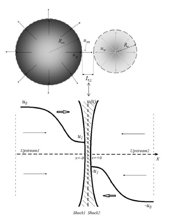
Figure 1: Simplified scheme of velocity profiles for the approaching shocks system.

where $D(x,p)$ is the diffusion coefficient, $u(x)$ is the fluid velocity. Integrating Eq. 2 from $x=-x_{0}$ to $x=x_{0}$ and splitting integration region into 3 parts: from $x=-x_{0}$ to $x=0^{-}$, from $x=0^{-}$ to $x=0^{+}$ and from $x=0^{+}$ to $x=x_{0}$, one can achieve the following equation

$$\frac{1}{3}p\frac{\partial}{\partial p}\left[\int_{-x_{0}}^{0^{-}}+\int_{0^{+}}^{x_{0}}\right]f\frac{du(x)}{dx}dx+\left[\int_{-x_{0}}^{0^{-}}+\int_{0^{+}}^{x_{0}}\right]f\frac{du(x)}{dx}dx+$$

$$+2(\phi_{esc}(p)-\frac{1}{3}p\frac{\partial f_{0}}{\partial p}u_{1})+Q_{0}(p)=0,$$ (3)

where $f_{0}(p)=f(x=0,p)$ is the distribution function at the shock, $Q_{0}(p)=Q(0,p)$ is the injection rate at the shock and $\phi_{esc}(p)=-\left[D(x,p)\frac{\partial f}{\partial x}\right]_{-x_{0}}$ is the escaping flux of energetic particles at $x=-x_{0}$ and $x=x_{0}$.

Assuming the symmetry of the shock flow profiles and introducing

$$u_{p}=u_{1}-\frac{1}{f_{0}(p)}\int_{-x_{0}}^{0}dx(du/dx)f(x,p)\ ,$$ (4)

where $u_{1}$ is the fluid velocity immediately upstream (at $x=0^{-}$ and $x=0^{+}$), we obtain:

$$p\frac{\partial f_{0}}{\partial p}=-\frac{3}{u_{p}}\left\{f_{0}\left(u_{p}+\frac{1}{3}p\frac{\partial u_{p}}{\partial p}\right)-\phi_{esc}(p)-\frac{1}{2}Q_{0}(p)\right\}.$$ (5)

The function $u_{p}$ is instrumental to account for the nonlinear modification of the flow due to backreaction of the accelerated particles and it is included into the non-linear calculations (for details see e.g. Amato & Blasi, 2005).

Thus the distribution function can be evaluated as

$$f_{0}(p)=\int_{p_{inj}-0}^{p}\frac{d\overline{p}}{\overline{p}}\frac{3(\phi_{esc}(\overline{p})+Q_{0}(\overline{p})/2)}{u_{\overline{p}}}\,K(p,\overline{p}),$$ (6)

where

$$K(p,\overline{p})=\exp\left[-\int_{\overline{p}}^{p}\frac{dp^{{}^{\prime}}}{p^{{}^{\prime}}}\frac{3}{u_{p^{{}^{\prime}}}}(u_{p^{{}^{\prime}}}+\frac{1}{3}p^{{}^{\prime}}\frac{\partial u_{p^{{}^{\prime}}}}{\partial p^{{}^{\prime}}})\right].$$ (7)

The CR injection rate in Eq. (2) can be written as

$$Q(x,p)=\frac{\eta n_{gas,1}u_{1}}{4\pi p_{inj}^{2}}\delta(p-p_{inj})\delta(x),$$ (8)

where $p_{inj}$ is particle injection momentum, $n_{gas,1}=\rho_{0}u_{0}/m_{p}u_{1}$ is the gas density immediately upstream ($x=0^{-}$ and $x=0^{+}$), $n_{0}$ and $\rho_{0}$ are gas density and mass density at the shock and $\eta$ is the fraction of the particles which are considered to be injected into the acceleration process. Hence, $f_{0}(p)$ can be presented in a simple form

$$f_{0}(p)=\frac{3\eta\rho_{0}}{8\pi m_{p}U_{p}(p)}\frac{1}{p^{3}}-\frac{3}{U_{p}(p)p^{3}}\int_{p_{0}}^{p}\phi_{esc}\,p^{{}^{\prime}2}dp^{{}^{\prime}},$$ (9)

where $U_{p}\equiv u_{p}/u_{0}$.

Eq. (9) represents the momentum distribution function at the high-energy limit ($\Lambda(p)>L_{12}$) for the MHD flow with two identical colliding shocks with the FEBs. Note, that for every momentum $p$ function $f_{0}(p)$ is proportional to $p^{-3}$ with correction factor $U_{p}(p)$. The first term in Eq. (9) reflects CR injection and the second term is due to the escaping flux. The second term is most important for the CR spectral shape at the highest energies (i.e. above $p>p_{\star}$ where $\Lambda(p_{\star})=L_{12}$). Such a simple form of the CRs distribution function can be obtained in the case of the symmetric flow. The corresponding expression for the general case is somewhat more complex and will be discussed elsewhere.

3 An approximate solution of diffusion-advection equation

In this section we use an approximate solution of the one-dimensional diffusion-advection equation proposed by Caprioli et al. (2010) with the distribution function at the shock $f_{0}(p)$ for the case of two converging shocks derived in the previous section. The solution was obtained by integrating the diffusion-convection equation from $-x_{0}$ to an arbitrary point $x$ in the shock upstream, with the FEB condition as given by Eq. (1). A symmetric model is considered, so that the solution in the upstream region $1$ ($x<0$) does not differ from the solution in the upstream region $2$ (see Fig. 1). Following Caprioli et al. (2010) we used an approximation of the exact solution to the transport equation

$$f(x,p)=f_{0}\exp\left[-\int_{x}^{0}dx^{\prime}\frac{u(x^{\prime})}{D(x^{\prime},p)}\right]\left[1-\frac{W(x,p)}{W_{0}(p)}\right],$$ (10)

$$\phi_{esc}(p)=-\frac{u_{0}f_{0}}{W_{0}(p)}\,,$$ (11)

where $D(x,p)$ is the CR diffusion coefficient,

$$W(x,p)=u_{0}\int_{x}^{0}dx^{\prime}\frac{\exp\left[-\psi(x^{\prime},p)\right]}{D(x^{\prime},p)},$$ (12)

$$\psi(x,p)=-\int_{x}^{0}dx^{\prime}\frac{u(x^{\prime})}{D(x^{\prime},p)}\ ,$$ (13)

and $W_{0}(p)=W(x_{0},p)$.

These expressions are exact in the test-particle limit, as one can easily verify. The iterative method that has been used in the calculations is based on the successive approximations to the solution $f(x,p)$ that satisfy both the CR transport and the momentum-energy conservation equations. The momentum conservation equation, normalized to $\rho_{0}u_{0}^{2}$ reads

$$U(x)+P_{c}(x)+P_{w}(x)+P_{g}(x)=1+\frac{1}{\gamma M_{0}^{2}}\,,$$ (14)

where $M_{0}$ is the Mach number of the unperturbed flow. The normalized cosmic ray pressure

$$P_{c}(x)=\frac{4\pi}{3\rho_{0}u_{0}^{2}}\int_{p_{inj}}^{\infty}dp~{}p^{3}~{}v(p)~{}f(x,p)\,,$$ (15)

where $v(p)$ is the velocity of the particle. The normalized pressure of magnetic fluctuations generated via the resonant streaming instability (see Eq.(42) in Caprioli et al., 2009)

$$P_{w}(x)=\frac{v_{A}}{4u_{0}}\frac{1-U^{2}(x)}{U^{3/2}(x)},$$ (16)

where $v_{A}=B_{0}/\sqrt{4\pi\rho_{0}}$ - is the Alfven velocity, $B_{0}$ - is the strength of the unperturbed magnetic field. Equation  (16) was obtained from the stationary equation for growth and transport of magnetic turbulence. We used the approximation for the turbulent energy flux $F_{w}(x)\simeq 3u(x)p_{w}(x)$, assuming that $v_{a}\ll u(x)$ (see, e.g., Caprioli et al., 2009). The normalized pressure of the background gas

$$P_{g}(x)=\frac{U^{-\gamma}(x)}{\gamma M_{0}^{2}}\,,$$ (17)

where $U(x)=u(x)/u_{0}$ and $\gamma$ is the adiabatic index.

The first iteration starts from a guess value for $U_{1}=u_{1}/u_{0}$, which uniquely determines $P_{w1}$, $P_{g1}$ and $P_{c1}$ via Eqs. (16), (17) and (14).

To the first approximation we start with a test-particle guess for $f(x,p)$, properly normalized in order to account for the pressure $P_{c1}$, and calculate $P_{c}(x)$ from Eq. (15) and then $U(x)$ with Eq. (14). Then the updated velocity profile is used to construct a new $P_{w}(x)$ and $\delta B(x)=\sqrt{8\pi\rho_{0}u_{0}^{2}P_{w}(x)}$ which is employed to update the diffusion coefficient $D(x,p)=v\,p\,c/3e\,\delta B(x)$.

According to Eq. (10), a new profile of $f(x,p)$ is obtained with the initial distribution function and the new $U(x)$ and $D(x,p)$. The procedure is iterated until a convergence is reached, i.e. until the remainders of $f(x,p)$ and its normalization factor reach a preset accuracy between two steps.

For an arbitrary value of $U_{1}$ with the fixed list of the model parameters, however, the required normalization factor can differ from 1, then the process is restarted with another choice of $U_{1}$ until no further normalization is needed. The distribution function calculated with the value of $U_{1}$ obtained by this approach is, by construction, the solution of both diffusion-convection and conservation equations for the two shock flow model.

In Fig. 2 we illustrate the CR spectrum in the limit of small $L_{12}$ when the shocks are colliding. The proton distribution function at the shocks (dotted line) given by Eqs. (9)-(10) and the corresponding escaping flux (dashed line) given by Eq. (11) were calculated with the semi-analytical approach. The following parameters were chosen for the calculation: the shock velocity $u_{0}=3,000~{}\rm~{}km~{}s^{-1}$, the free escape boundary is at $1.0$ pc on the both sides from the shocks, the background gas density is $n_{0}=1.0~{}\rm~{}cm^{-3}$ and the Alfven velocity is $v_{A}=30~{}\rm~{}km~{}s^{-1}$. Within the spectrum calculation we used the diffusion coefficient $D(x,p)$=5$\times$10${}^{20}\,\,[p/(GeV/c)]\times(\delta B(x)/100\mu G)^{-1}$ $\rm~{}cm^{2}~{}s^{-1}$. The ratio of the escaping and injection fluxes is governed by the value of the diffusion coefficient in the upstream region $D(x,p)$, and in the model it is given by the expression

$$\frac{\phi_{esc}(p)}{u_{0}f_{0}(p)}=\frac{1}{W_{0}(p)}.$$ (18)

At the maximal momenta of the accelerated particles the dimensionless ratio Eq. (18) scales as $D(x_{0},p)$.

Figure 2: The CR proton spectrum $p^{3}f_{0}(p)$ at the shock position (dotted line) and the escaping flux $p^{3}\phi_{esc}(p)/u_{0}$ (dashed line), simulated in the non-linear semi-analytical model of DSA in the colliding shock flow

Note that the proton spectrum at the shock is not strongly modified by the cosmic ray pressure and differs from the case of a single modified shock simulated by Caprioli et al. (2010) with the same injection parameter $\xi_{inj}=3.3$, corresponding to a fraction of injected particles $\eta\simeq 1.2\times 10^{-3}$.

It is worth noting that the spectral shape of the escaping CR flux (showed as the dashed line in Fig. 2) differs from that in the case of a single strong shock. In the case of the approaching shocks flow the escaping particles form a flattened spectra at lower energies. The spectral shape is no longer symmetric and it departs from the parabolic law.

In the case of a SN shock approaching a termination shock of the stellar wind, the system is non-steady. Nevertheless, one can make use of the non-linear steady solution given above to simulate the instant flow profiles between the shocks, provided the CR acceleration time $\tau_{a}$ is short compared the dynamical time scale $\tau_{\rm dyn}=L_{12}/u_{sn}$, where $u_{sn}$ is the velocity of the SNR forward shock. The simulated instant profiles can be then implemented into the non-steady transport equations for CR protons and electrons to account for the time-dependent position of the approaching shocks.

It is important to note that the plasma flow in between the converging shocks is governed by the gradient of the CR pressure. The CR pressure itself may be dominated by the highest energy part of the CR spectra. However, the CR protons of momenta $p>p_{\star}$ propagate in between the shocks without scattering, and their pressure is nearly homogeneous. In result, the flow is modified by the pressure gradient of the CR particles with $p<p_{\star}$. These have the acceleration time shorter than $\tau_{\rm dyn}$ and are mainly concentrated in the vicinity of the shocks.

4 Time-dependent model simulations

The non-linear modification of the colliding shock flow by the accelerated cosmic ray pressure can be accounted for within a time-dependent model. A specific feature of the simulation is that the highest energy CRs of $p_{\rm max}\geq p\;\raise 1.29167pt\hbox{$>$\kern-7.5pt\raise-4.73611pt\hbox{$\sim$}}\;p_{\star}$ propagate without scattering, but their momenta are still nearly isotropic being scattered in the extended shock downstream regions. To treat the case one can use the transport equation in the form of the telegraph equation. The telegraph equation can be derived from the Boltzmann kinetic equation for a nearly-isotropic CR particle distribution (see, e.g., Eq.(35) in Earl, 1974). The equation allows a smooth transition between the diffusive and the scatter-free propagation regimes. With time-dependent simulations we calculated the energy spectra of cosmic ray protons and electrons at a SNR shock approaching a strong wind of a nearby early type star. For relativistic electrons/positrons we account for the energy losses due to synchrotron and inverse Compton (IC) radiation.

We solve one-dimensional transport equations for the pitch-angle-averaged phase space distribution function of protons, $f_{p}(x,p,t)$, and electrons, $f_{e}(x,p,t)$, given by

$$\tau(p)\frac{\partial^{2}g_{p}}{\partial t^{2}}+\frac{\partial g_{p}}{\partial t}+u(x)\frac{\partial g_{p}}{\partial x}-\frac{1}{3}\frac{\partial u(x)}{\partial x}\left(\frac{\partial g_{p}}{\partial y}-4g_{p}\right)=$$

$$\frac{\partial}{\partial x}\left(D(x,p)\frac{\partial g_{p}}{\partial x}\right),$$ (19)

$$\tau(p)\frac{\partial^{2}g_{e}}{\partial t^{2}}+\frac{\partial g_{e}}{\partial t}+u(x)\frac{\partial g_{e}}{\partial x}-\frac{1}{3}\frac{\partial u(x)}{\partial x}\left(\frac{\partial g_{e}}{\partial y}-4g_{e}\right)=$$

$$\frac{\partial}{\partial x}\left(D(x,p)\frac{\partial g_{e}}{\partial x}\right)+\exp(y)\frac{\partial}{\partial y}\left[b\exp(-2y)g_{e}\right],$$ (20)

where $g_{p}=p^{4}f_{p}$, $g_{e}=p^{4}f_{e}$, $y=ln(p)$. The dimensionless particle momentum $p$ is expressed in the units of $m_{p}c$. The cooling term $b(p)=-dp/dt$ describes the electron synchrotron and IC losses (see, e.g., Kang, 2011). Here $\tau(p)=\Lambda(p)/v$ is a CR particle pitch-angle scattering mean free time. The transport equations Eq.  (4) and Eq.  (20) are modified telegraph equations (see, e.g., Earl, 1974; Toptygin, 1985). The telegraph equation embodies both the diffusive propagation of low energy particles $p<p_{\star}$ with the mean free paths below $L_{12}$ and the ballistic scatter free propagation of particles with $p\;\raise 1.29167pt\hbox{$>$\kern-7.5pt\raise-4.73611pt\hbox{$\sim$}}\;p_{\star}$. The transport equations are valid for nearly isotropic particle distributions that can be maintained for particles with momenta $p_{\rm max}\geq p\;\raise 1.29167pt\hbox{$>$\kern-7.5pt\raise-4.73611pt\hbox{$\sim$}}\;p_{\star}$ that are scattered in the inflowing plasma (Upstream 1 and 2 regions shown in Fig. 1). At high energies $p\;\raise 1.29167pt\hbox{$>$\kern-7.5pt\raise-4.73611pt\hbox{$\sim$}}\;p_{\star}$ the ballistic propagation of CR particles in between the shocks is governed by the first terms of the transport equations. The diffusion coefficient in the regime saturates at $D_{is}\approx cL_{12}$.

At the moving shocks we applied the standard matching conditions used in DSA (see, e.g., Bell, 1978; Blandford & Eichler, 1987). The matching conditions are equating the isotropic parts of the distribution functions and the particle fluxes in the phase space at the shock surface to guarantee the particle number conservation. At the simulation box boundaries $x=\pm x_{b}$ we used the free escape boundary conditions $g_{i1}(t,-x_{b},p)=0$ and $g_{i2}(t,x_{b},p)=0$. The simulation starts with the initial test particle distribution function at the shocks $dN(p)/dp\sim 1/p^{2}$ and $\partial{N}/\partial{t}=0$ at $t=0$.

The transport equations were solved with integration-interpolation algorithm and the standard Crank-Nicolson scheme. The model allows to calculate $f_{e,p}(x,p,t)$ at any position between the shocks and in the post-shock flows.

In Fig. 3 (left panels) we present the result of calculations of the proton distribution function. This was obtained in the time-dependent model simulations of the flow between colliding shocks. Four panels display $f_{p}(x,p,t)$ in the phase space $(p,x)$ at four different times which correspond to the inter-shock distances of 0.6 pc, 0.5 pc, 0.3 pc and 0.1 pc. The free escape conditions are applied at the simulation box boundary at $x_{b}$ = 0.55 pc. At each time step the flow model implements the modified velocity profiles, u(x,t), obtained in the semi-analytical iteration scheme described in paragraph §3. The four right panels in Fig 3 show the proton and electron spectra, $dN_{p}(p)/dp$ and $dN_{e}(p)/dp$, at the moving left shock, at the corresponding time moments, compared to the expected spectrum $dN/(p)/dp\propto 1/p$. In Fig. 3 the spectral evolution of CRs is clearly seen. Initially, the CR protons are concentrated around the shocks, and the proton spectrum is close to the spectrum of the isolated SNR shock, $dN_{p}(p)/dp\propto 1/p^{2}$. As the inter-shock distance reduces, the proton spectrum gets harder and the CRs concentrate in between the shocks. At the distance of 0.1 pc, the spectrum of CR protons accelerated in the two-shocks system almost coincides with the spectrum $dN(p)/dp\propto 1/p$.

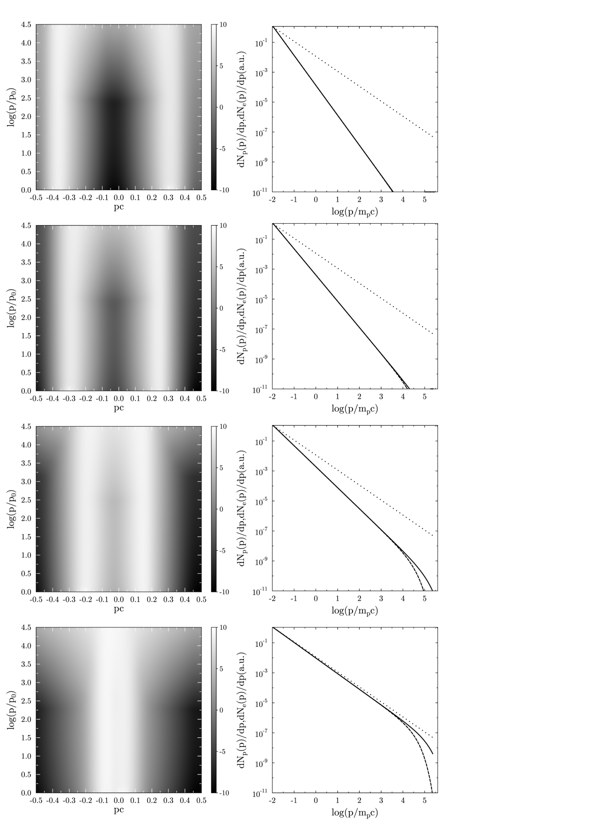
Figure 3: On the left: the proton distribution function $f(x,p)\,p^{3}$ (gray scaled) as a function of the CR momentum and the position $x$, presented for four different distances between the shocks - from top to bottom: 0.6 pc, 0.5 pc, 0,3 pc, 0.1 pc. The left shock is propagating in the positive direction of the $x$- axis and the right shock is moving in the opposite direction. The shock velocities are 3,000 $\rm~{}km~{}s^{-1}$. On the right: the proton and electron spectra at the moving left shock for the times corresponding to the four intershock distances given above. Solid line - simulated proton spectrum $dN_{p}/dp$, dashed line - simulated electron spectrum $dN_{e}/dp$ multiplied by a factor of 100 for the clarity of presentation. The asymptotic spectral shape $dN/dp\propto 1/p$ is shown with dotted line.

The later result is consistent with the expectation that for the efficient acceleration process in such a system, the acceleration time for the highest energy particles, $\tau_{a}$, should be comparable to the dynamical time $\tau_{\rm dyn}$. The condition is satisfied if: (i) $u_{sn}L_{12}>3\cdot D_{sn}$ and $u_{sn}L_{12}>3\cdot D_{sw}$, where $u_{sn}$ - velocity of the SNR shock, $D_{sn}$ and $D_{sw}$ - the Bohm-type diffusion coefficients for the supernova and the stellar wind shocks correspondingly (see Bykov et al., 2011), (ii) the diffusion coefficient in the interstellar medium between the shocks $D_{is}\gg D_{sn},D_{sw}$. We did not model here the magnetic field amplification process, but rather parameterized the Bohm diffusion coefficients relying on the simulations of DSA magnetic field amplification at a single shock performed by Vladimirov et al. (2008). Assuming that the amplified magnetic field near the shock is $\sim 100$ $\mu G$ as it was inferred from young SNR observations recently reviewed by Vink (2012), the distance between the shock fronts $L_{12}\sim 1$ pc, we used $D_{is}=100\times D_{sn}$ and $D_{sw}\simeq D_{sn}$ for the Bohm-type diffusion.

5 Discussion

The simplified non-linear model of particle acceleration in a converging flow between a young supernova shell and a fast wind of a massive early type star predicts a hard spectrum of CR protons confined in the flow and CRs escaping the accelerator of about a decade width in energy as shown in Fig. 2. In the considered case of the SNR shock and wind velocities of $\sim 3,000~{}\rm~{}km~{}s^{-1}$ and about a parsec distance between the shocks the maximal energies accelerated protons can reach 10⁵ GeV. The energy is close to the expected DSA limit in an isolated supernova shock (see e.g. Lagage & Cesarsky, 1983; Hillas, 2005). In individual SNRs the maximal energy depends strongly on the circumstellar matter of the SN progenitor and the maximal energy of the accelerated CRs can be reached typically at the early Sedov phase. It is important that if SNR is expanding in a cluster of young massive stars both the maximal energy and the flux of the escaping accelerated CRs may be non-monotonous functions of the SN age, and may have secondary maxima at the moments of close approaches of the SNR and fast stellar winds. It should be noted that massive shells that are surrounding the stellar winds (see e.g. Lamers & Cassinelli, 1999) may be swept away by the first few SN explosions in a compact cluster of young massive stars, thus alleviating the collisions of supernova shells with the wind termination shocks. The stage of the closely approaching SNR and stellar wind flows that is favorable for particle acceleration typically lasts for 300-1,000 years depending on the stellar wind velocity and the termination shock radius. Therefore, such sources can likely contribute to the galactic CRs population. The colliding supersonic flows with two shocks also occur in the early-type runaway stars. Particle acceleration in a way similar to that discussed above may occur in between the bow-shock and the wind termination shock of a fast runaway early type star. Recently a bow-shock survey with 28 fast runaway OB stars was compiled by Peri et al. (2012) providing candidate source for particle accelerators. The velocities of runaway early type stars are well below that of the supernova shocks discussed above and therefore the maximal energies of accelerated particles are expected to be lower than that in SNR-SW collision. However the fast runaway early type stars may still be sources of non-thermal emission with hard photon spectra.

Figure 4: Model spectral energy distribution (SED) of the inverse Compton emission from electrons accelerated at the colliding shock flow (solid line) to compare with the emission of the electrons accelerated by a single isolated shock of the same speed (dashed line). The SEDs are given in arbitrary units and calculated for the intershock distance of 0.1 pc. The corresponding distribution function of the IC emitting electrons is shown in the bottom panel in Fig. 3

The simplified non-linear model discussed in the paper predicts a hard high energy end of CR particle spectrum. The simulated spectrum of electrons is shown in Fig. 3 (dashed curve). The shape of the electron spectrum is similar to that of protons, but the synchrotron/IC cooling effects result in the spectrum cut-off at lower energies. The electromagnetic radiation produced by hard spectra of electron/positron confined in the accelerator can be potentially observed, thus constraining the physical parameters of the observed objects. In Fig. 4 we present a model spectrum of the inverse Compton (IC) emission from the electrons accelerated in a colliding shock flow comparing to the IC spectrum of a single shock flow modeled earlier (see e.g. Gaisser et al., 1998; Baring et al., 1999; Bykov et al., 2000). To construct the IC spectrum we used the same emission model which was applied to model high energy emission of the supernova remnant IC 443 described in detail in Bykov et al. (2000). SNR IC 443 is likely located in Gem OB1 - young massive star association. Therefore in addition to the local interstellar photon spectrum which following Mathis et al. (1983) was approximated by the sum of diluted blackbody spectra with temperatures 2.7 K, 7500 K, 4000 K and 3000 K a major infrared component resulting from the dust heated in OB association must be accounted for. In the vicinity of IC 443 according to IRAS observations of Saken et al. (1992) we approximated the infrared component with two temperatures fit (185 K and 34.3 K components). If the shock collision region is located at the distance further than about 2 parsecs from the young massive star then the UV emission of the star does not dominate the IC losses of relativistic electrons.

The electron distribution used in the IC spectrum computation is shown in the bottom panel in Fig. 3. The electron/positron distribution function $f_{e}(x,p,t)$ was computed with the time-dependent model Eq.(20) that accounts for non-linear flow modification in the shocks vicinity as discussed in the previous section, and the electron synchrotron/IC losses included. It is clearly seen that due to the hard spectrum of accelerated electrons up to $10^{4}$ GeV the emissivity of the SNR-SW system is higher than that for the single SNR shock. TeV-sources with very hard spectra are not always easily identified with their GeV counterparts and some of these may comprise the population of so-called ”dark accelerators”. The prototype of the dark accelerators was TeV J2032+4130 discovered a decade ago by Aharonian et al. (2002), though the source is possibly associated with the pulsar 2FGL J2032.2+4126 detected later in GeV regime by Fermi observatory. Another high energy source was found by H.E.S.S. (see Abramowski et al., 2012a) in the vicinity of the young massive stellar cluster Westerlund 1. The sources originating in the colliding supersonic flows considered above may contribute to the VHE emission of young massive star associations (see, e.g., Bykov, 2001; Torres et al., 2004) and the star-burst galaxies that are also known to be bright gamma-ray sources (see, e.g., Abramowski et al., 2012b). The main goal of the paper is to discuss the unique features of particle accelerators associated with the colliding shock flows. To model the broadband non-thermal emission spectra of the sources one has to discuss in detail matter and magnetic field distributions in the complex flows. The structure of magnetic field in the winds of young massive stars is under study, see for a review Walder et al. (2012). In the IC spectra modeling we assumed that the CR electrons are the test particles that are propagating in the flow modified by the CR protons. We did not consider here any specific electron injection model to calculate their absolute fluxes and therefore the IC spectra in Fig. 4 are shown in arbitrary units. We will present a more detailed emission spectra modeling of colliding shock flows elsewhere.

Appendix A Momentum-Energy flux conservation

In this section we check the accuracy of the quasi-steady non-linear model used, since it is relying on an the approximation of the CR distribution function as given by Eq. (10). In a steady-state system, mass, momentum and energy fluxes must be constant in space obeying the following conservation laws

$$\rho(x)u(x)=\rho_{0}u_{0},$$ (21)

$$\Phi_{P}(x)=\rho_{0}u_{0}^{2}+P_{g0},$$ (22)

$$\Phi_{E}(x)=\Phi_{E0},$$ (23)

where $\rho$ and $u$ are the mass density and the flow velocity, $\Phi_{P}(x)$ and $\Phi_{E}(x)$ are the fluxes of the $x$-component of the momentum and energy in the $x$-direction. The index ”0” marks the far upstream values.

Figure 5: The energy conservation check. The shock velocity profile $U(x)$ is given for the flow of Mach number $M_{0}=100$. The shock is located at $x=0$ and the position of the free escape boundary is at $x=1.0$. The cosmic ray pressure $P_{c}(x)$, the pressure of the background gas $P_{g}(x)$ and the pressure of magnetic fluctuations $P_{w}(x)$ are normalized to $\rho_{0}u_{0}^{2}$. The energy flux $\Phi_{E}(x)$ is normalized to $\rho_{0}u_{0}^{3}$.

The CR energy and momentum fluxes are calculated from the CR distribution function. In the paper we assumed that the CR energy and momentum are dominated by protons, and the CR electrons are treated as test particles that are propagating in the flow modified by CR protons. A weakly anisotropic CR distribution function of the accelerated particles can be approximated as

$$f(\textbf{r},p)=\frac{1}{4\pi}\left[N(\textbf{r},p)+\frac{3}{v^{2}}\textbf{v}\textbf{J}(\textbf{r},p)\right],$$ (24)

where $N(\textbf{r},p)$ is the isotropic part of the distribution function, $\textbf{J}(\textbf{r},p)$ is the particles flux (e.g. Toptygin, 1985). The $x$-component of the flux can be written as:

$$J_{x}(x,p)=-D(x,p)\frac{\partial N}{\partial x}-\frac{p}{3}\frac{\partial N}{\partial p}u(x)\,.$$ (25)

The energy flux $\Phi_{cr}(x)$ is defined as

$$\Phi_{cr}(x)=\int K(p)v_{x}(p)f(x,p)d^{3}p\,,$$ (26)

where $K(p)=E-mc^{2}$ is the kinetic energy of a particle, $E=\sqrt{(pc)^{2}+m^{2}c^{4}}$ is the full energy of the particle, $v_{x}=v\cdot cos\theta$, $\theta$ is the angle between the particle momentum and the $x$-axis, and $v=\frac{\partial E}{\partial p}$.

Substituting the $x$-component of the distribution function Eq. (24) into the equation Eq. (26), one can obtain

$$\Phi_{cr}(x)=\int\left[N(x,p)+\frac{3}{v}cos\theta J_{x}(x,p)\right]\,K(p)\,v\,cos\theta\,\frac{d^{3}p}{4\pi}.$$ (27)

Integrating over the angle one can get the CR energy flux

$$\Phi_{cr}(x)=\int_{0}^{\infty}\,K(p)\left[-D(x,p)\frac{\partial N}{\partial x}-\frac{p}{3}\frac{\partial N}{\partial p}u\right]p^{2}dp.$$ (28)

Then, finally, the expression for the CR kinetic energy flux is

$$\Phi_{cr}(x)=\int_{0}^{\infty}p^{2}dp\left[-D(x,p)\frac{\partial N}{\partial x}K(p)+(\frac{pv}{3}+K(p))Nu\right].$$ (29)

The energy flux of the magnetic turbulence is expressed by

$$\Phi_{w}(x)\simeq 3u(x)p_{w}(x),$$ (30)

where $p_{w}(x)=\rho_{0}u^{2}_{0}P_{w}(x)$ is the pressure of the magnetic turbulence generated via resonant streaming instability (see Eq. (16) and Caprioli et al. (2009)).

Therefore, the energy conservation law for the steady non-linear model can be written as

$$\Phi_{g}(x)+\Phi_{w}(x)+\Phi_{cr}(x)-\Phi_{esc}=\Phi_{E}(x),$$ (31)

$$\frac{1}{2}\rho(x)u^{3}(x)+3u(x)p_{w}(x)+\frac{\gamma}{\gamma-1}u(x)p_{g}(x)+\Phi_{cr}(x)=const$$ (32)

where $\Phi_{cr}(x)$ is calculated from Eq. (29),

$$p_{g}(x)=\rho_{0}u^{2}_{0}P_{g}(x)$$

is the pressure of the background gas and

$$\Phi_{esc}=\int_{p_{inj}}^{\infty}E\cdot\phi_{esc}(p)dp$$

is the energy flux of the escaping CRs.

In Figure 5 we illustrate the accuracy of the energy conservation in the employed model of particle acceleration. The dimensionless spatial coordinate is normalized to the FEB position distance $x_{0}$. The energy flux conservation accuracy is about $1\%$. Some small inconstancy of the full energy flux can be attributed to the particular choice of the approximation of the CR distribution function given by Eq. (10) that was used in the non-linear model.

References

- Abramowski et al. (2012a) Abramowski A., et al. 2012a, A&A, 537, A114
- Abramowski et al. (2012b) Abramowski A., et al. 2012b, ApJ, 757, 158
- Ackermann et al. (2011) Ackermann M., et al., 2011, Science, 334, 1103
- Aharonian et al. (2002) Aharonian F., et al. 2002, A&A, 393, L37
- Aharonian et al. (2012) Aharonian F., Bykov A., Parizot E., Ptuskin V., Watson A., 2012, Space Sci. Rev., 166, 97
- Amato & Blasi (2005) Amato E., Blasi P., 2005, MNRAS, 364, L76
- Axford et al. (1977) Axford W. I., Leer E., Skadron G., 1977, in 15th International Cosmic Ray Conference, Plovdiv, Vol. 11 , pp 132–137
- Baring et al. (1999) Baring M. G., Ellison D. C., Reynolds S. P., Grenier I. A., Goret P., 1999, ApJ, 513, 311
- Bell (1978) Bell A. R., 1978, MNRAS, 182, 147
- Bell (1987) Bell A. R., 1987, MNRAS, 225, 615
- Bell (2004) Bell A. R., 2004, MNRAS, 353, 550
- Berezhko & Krymskii (1988) Berezhko E. G., Krymskii G. F., 1988, Sov. Phys. Uspekhi, 31, 27
- Blandford & Eichler (1987) Blandford R., Eichler D., 1987, Phys. Reports, 154, 1
- Blandford & Ostriker (1978) Blandford R. D., Ostriker J. P., 1978, ApJ, 221, L29
- Blasi (2004) Blasi P., 2004, Astroparticle Physics, 21, 45
- Bykov (2001) Bykov A. M., 2001, Space Science Reviews, 99, 317
- Bykov et al. (2000) Bykov A. M., Chevalier R. A., Ellison D. C., Uvarov Y. A., 2000, ApJ, 538, 203
- Bykov et al. (2011) Bykov A. M., Gladilin P. E., Osipov S. M., 2011, MemSAIt, 82, 800
- Bykov et al. (2011) Bykov A. M., Osipov S. M., Ellison D. C., 2011, MNRAS, 410, 39
- Bykov & Toptygin (2001) Bykov A. M., Toptygin I. N., 2001, Astronomy Letters, 27, 625
- Caprioli et al. (2010) Caprioli D., Amato E., Blasi P., 2010, Astroparticle Physics, 33, 307
- Caprioli et al. (2009) Caprioli D., Blasi P., Amato E., Vietri M., 2009, MNRAS, 395, 895
- Drury & Völk (1981) Drury L. O., Völk J. H., 1981, ApJ, 248, 344
- Earl (1974) Earl J. A., 1974, ApJ, 188, 379
- Eichler & Usov (1993) Eichler D., Usov V., 1993, ApJ, 402, 271
- Ferrand & Marcowith (2010) Ferrand G., Marcowith A., 2010, A&A, 510, A101
- Gagné et al. (2011) Gagné M., et al. 2011, ApJS, 194, 5
- Gaisser et al. (1998) Gaisser T. K., Protheroe R. J., Stanev T., 1998, ApJ, 492, 219
- Hillas (2005) Hillas A. M., 2005, Journal of Physics G Nuclear Physics, 31, 95
- Jones & Ellison (1991) Jones F. C., Ellison D. C., 1991, Space Science Reviews, 58, 259
- Kang (2011) Kang H., 2011, Journal of Korean Astronomical Society, 44, 49
- Krymskii (1977) Krymskii G. F., 1977, Akademiia Nauk SSSR Doklady, 234, 1306
- Lagage & Cesarsky (1983) Lagage, P.O., and Cesarsky, C.J., 1983, A&A,, 118, 223
- Lamers & Cassinelli (1999) Lamers H. J. G. L. M., Cassinelli J. P., Introduction to Stellar Winds, Cambridge University Press, 1999
- Malkov & O’C Drury (2001) Malkov M. A., O’C Drury L., 2001, Reports on Progress in Physics, 64, 429
- Mathis et al. ( 1983) Mathis J. S., Mezger P. G.,Panagia N. 1983,A&A, 128, 212
- Peri et al. (2012) Peri C. S., Benaglia P., Brookes D. P., Stevens I. R., Isequilla N. L., 2012, A&A, 538, A108
- Pittard & Dougherty (2006) Pittard J. M., Dougherty S. M., 2006, MNRAS, 372, 801
- Ptuskin et al. (2010) Ptuskin V., Zirakashvili V., Seo E.-S., 2010, ApJ, 718, 31
- Reville et al. (2009) Reville B., Kirk J. G., Duffy P., 2009, ApJ, 694, 951
- Saken et al. (1992) Saken J. M., Fesen R. A., Shull J. M., 1992, ApJS, 81, 715
- Schure et al. (2012) Schure K. M., Bell A. R., O’C Drury L., Bykov A. M., 2012, Space Sci. Rev., 173, 491
- Toptygin (1985) Toptygin I. N., Cosmic rays in interplanetary magnetic fields, Reidel, 1985
- Torres et al. (2004) Torres D. F., Domingo-Santamaría E., Romero G. E., 2004, ApJ, 601, L75
- Vink (2012) Vink J., 2012, Astron. Astroph. Reviews, 20, 49
- Vladimirov et al. (2008) Vladimirov A. E., Bykov A. M., Ellison D. C., 2008, ApJ, 688, 1084
- Walder et al. (2012) Walder R., Folini D., Meynet G., 2012, Space Sci. Rev., 166, 145
- Wright et al. (2010) Wright N. J., Drake J. J., Drew J. E., Vink J. S., 2010, ApJ, 713, 871