Estimation of the neutrino flux and resulting constraints on hadronic emission models for Cyg X-3 using AGILE data

P. Baerwald and D. Guetta^,

Institut für Theoretische Physik und Astrophysik, Universität Würzburg,

D-97074 Würzburg, Germany

Osservatorio astronomico di Roma, v. Frascati 33,

I-00040 Monte Porzio Catone, Italy

Department of Physics and Optical Engineering, ORT Braude, P.O. Box 78,

Carmiel, Israel

Abstract

In this work we give an estimate of the neutrino flux that can be expected from the microquasar Cyg X-3. We calculate the muon neutrino flux expected here on Earth as well as the corresponding number of neutrino events in the IceCube telescope based on the so-called hypersoft X-ray state of Cyg X-3. If the average emission from Cyg X-3 over a period of 5 yr were as high as during the used X-ray state, a total of 0.8 events should be observed by the full IceCube telescope. We also show that this conclusion holds by a factor of a few when we consider the other measured X-ray states. Using the correlation of AGILE data on the flaring episodes in 2009 June and July to the hypersoft X-ray state we calculate that the upper limits on the neutrino flux given by IceCube are starting to constrain the hadronic models, which have been introduced to interpret the high-energy emission detected by AGILE.

1 Introduction

One of the fundamental questions in astrophysics is if hadrons are present in the jets of astrophysical sources like microquasars (MQs), quasars, and gamma-ray bursts (GRBs). This is still an open issue not solved by the detection of photons or high-energy protons (who lose information on the originating source on their way from the source to us). Unlike high-energy photons and protons, neutrinos can travel cosmological distances without being absorbed or deflected. Therefore, neutrinos can provide information on astrophysical sources that cannot be obtained with high-energy photons and charged particles. However the weak interaction of neutrinos with matter also implies that they are very difficult to detect, requiring detectors with an instrumented volume of $\mathcal{O}(\mathrm{k}\mathrm{m}\mathrm{{}^{3}})$. IceCube, completed in 2010 December, is the first kilometer-scale neutrino detector. IceCube analyses include model-independent searches for a diffuse flux and searches for point sources. Recent efforts to detect higher energy neutrinos from sources outside our solar system yield important constraints on point sources and diffuse fluxes of possible sources in the Galaxy (Abbasi et al. (2013)).

In this paper, we concentrate on one kind of astrophysical sources with relativistic jet, MQs. These are Galactic X-ray binary systems, which exhibit relativistic radio jets (Mirabel & Rodriguez (1999); Fender (2001)). These systems are believed to consist of a compact object, a neutron star or a black hole, and a giant star companion. Mass transfer from the giant star to the compact object through the formation of an accretion disk and the presence of the jets make them similar to small quasars, hence their name “microquasars.” The observed radiation from MQ jets, typically is in the radio and in some cases also in the IR band and it is consistent with non-thermal synchrotron radiation emitted by a population of relativistic, shock-accelerated electrons. Recently high-energy emission, $\sim\mathrm{G}\mathrm{eV}$, has been detected from MQ by AGILE and Fermi.

MQs can also be sources of $1$–$100\,\mathrm{T}\mathrm{eV}$ neutrinos (Levinson & Waxman (2001)) that come from the interaction of $\sim 10^{16}\,\mathrm{eV}$ protons with synchrotron photons emitted by the shock-accelerated electrons. The predicted fluxes should be detectable by large, km²-scale effective area, high-energy neutrino telescopes, such as the operating south pole detector IceCube, see Ahrens et al. (2003). Distefano et al. (2002) have extended the work of Levinson & Waxman (2001) and predicted the neutrino flux for several MQs whose radio data were available in the literature. They found that the largest number of neutrinos from bursting MQs is expected to come from Cyg X-3 and XTE J1118 +480.

In this paper, we want to study the role of the hadronic component in the MQ jet on the high gamma-ray emission mechanism. In order to perform this analysis, we use the IceCube and AGILE data.

The AGILE team has made a detailed study of $\gamma$-ray emission from Cygnus X-3 with the AGILE satellite. The AGILE discovery of transient $\gamma$-ray emission from Cygnus X-3 in 2008 April associated with a specific spectral state preceding a major radio jet ejection opened a new window of investigation of MQs. Several other major $\gamma$-ray emission episodes from Cygnus X-3 have been detected by AGILE and Fermi since 2008 (Tavani et al. (2009); Fermi LAT Collaboration et al. (2009)). The AGILE discovered several transient $\gamma$-ray emission episodes from Cygnus X-3 in the energy range $100\,\mathrm{M}\mathrm{eV}$ – $50\,\mathrm{G}\mathrm{eV}$ during the periods 2009 June–July and 2009 December–2010 mid-June. They found that the $\gamma$-ray emission from Cygnus X-3 is detectable by AGILE not only during relatively short (1–2 days) flares as in Tavani et al. (2009), but also during extended periods lasting several days or weeks (as during 2009 June–July; Bulgarelli, A. et al. (2012)). Detecting continuous $\gamma$-ray emission during “active” phases is of great theoretical relevance for the modeling of Cygnus X-3.

The main mechanism at the origin of the high-energy emission detected by AGILE can be the inverse Compton (IC) scattering of high-energy electrons accelerated in the source with low-energy photons emitted by synchrotron process (Dubus et al. (2010)). However, another possibility, if hadrons are present in the jet, is that the $100\,\mathrm{M}\mathrm{eV}$–$50\,\mathrm{G}\mathrm{eV}$ emission is due to $\pi^{0}$ decay into $\mathrm{T}\mathrm{eV}$ $\gamma$-rays that trigger a cascade to GeV gamma rays. These $\pi^{0}$ may be produced in the jet by photohadronic interactions or by proton–proton collisions between protons in the jet and protons in the gaseous surroundings provided by the WR companion mass outflow (Piano et al. (2012); Romero et al. (2003)).

In this paper, we use a simplified jet model to estimate the number of neutrinos expected from Cyg X-3 based on the X-ray data taken in 2009 during an episode of flares. In Section 2, we describe the simplified model we use for the jet of the MQ and the photohadronic interactions happening inside of it. In Section 3, we derive the expected photon and proton densities inside the jet of Cyg X-3, which are needed for the simulation of the photohadronic interactions, from the observed X-ray data. In Section 4, we then use the derived densities to estimate the expected neutrino number both in the case that the emission is due to IC and in the case that is due to $\pi^{0}$ decay into $\gamma$-ray photons. In Section 5, we discuss our results.

2 A simplified jet model

In this section, we want to describe our simplified jet model. The model we want to apply to the MQ Cyg X-3 was originally used for GRB which are also assumed to originate from emitting jets. The main simplification is that we totally neglect the dynamic of the propagating jet and assume that the outflow is static. The high-energy protons as well as the X-ray and $\gamma$-ray photons are assumed to be present in one interaction zone and emission will only originate from this one emission region. Both the proton as well as the photon density are assumed to be isotropic in the plasma rest frame of the jet. These assumptions are essential for us to use the photohadronic interaction code based on Hümmer et al. (2010b) (model Sim-B), which is an analytical parameterization based on SOPHIA, see Mücke et al. (2000). Starting from the particle densities, the code calculates the result of the photohadronic interactions leading to secondary particles which subsequently decay into neutrinos. It is based on an analytical parameterization of the full photohadronic interaction cross section and includes features, such as individual treatment of secondary particles, helicity-dependent muon decay, as well as neutrino flavor mixing, for details see Hümmer et al. (2010a). With this treatment we also incorporate the magnetic field effects discussed by Reynoso & Romero (2009), which do play a role due to the assumption of neutrino production in the internal shocks.

We assume in concordance with Levinson & Waxman (2001) that the photon energy density inside the jet $U^{\prime}_{\gamma}$ can be calculated from the emitted luminosity $L$ of the source by considering the emission passing the surface of the jet

$$U^{\prime}_{\gamma}=\frac{L}{4\pi\,\left(l^{2}\cdot\sin^{2}(\theta_{j})\right)\,c\,\mathcal{D}^{2}}$$ (1)

with $l$ being the distance of the emission region from the central object, $\mathcal{D}$ being the Doppler factor of the jet, and $\theta_{j}$ being the opening angle of the jet. Note that the boost with the Doppler factor is needed, since $U^{\prime}_{\gamma}$ is the energy density inside the shock frame. Additionally, we know that the photon energy density can be defined as

$$U^{\prime}_{\gamma}=\int E^{\prime}_{\gamma}\,n^{\prime}_{\gamma}\,\mathrm{d}E^{\prime}_{\gamma}\quad,$$ (2)

with $n^{\prime}_{\gamma}$ being the photon spectrum in particles per volume and per energy. For our photohadronic interaction calculation we will need $n^{\prime}_{\gamma}$. The shape of this spectrum can be obtained from the photon data, while the normalization can be obtained using Eq. (2).

Hence, by knowing the observed (energy integrated) photon flux $F_{\gamma}$ we can calculate the (isotropic equivalent) luminosity $L=4\pi\,D_{L}^{2}\,F_{\gamma}$, and subsequently the photon particle density inside the jet. Moreover, it is possible to calculate the energy carried by the magnetic field $B$ as well as the energy in protons from energy (equi-)partition arguments. These theoretical considerations need to be applied since we currently do not have the possibility to estimate the magnetic field strength by other means. Following the considerations of Levinson & Waxman (2001), it is possible to estimate the magnetic field $B^{\prime}$ (in G) by

$$B^{\prime}=\sqrt{8\pi\,\frac{\varepsilon_{B}}{\varepsilon_{e}}\,U^{\prime}_{\gamma}}$$ (3)

with $\varepsilon_{B}$ being the fraction of the jets total energy carried by magnetic field, $\varepsilon_{e}$ being the fraction carried by electrons/photons, and $U^{\prime}_{\gamma}$ from Eq. (1) in $\text{erg}\,\reciprocal\mathrm{s}$. Accordingly, we can estimate that the energy density carried by protons is

$$U^{\prime}_{p}=\frac{\varepsilon_{p}}{\varepsilon_{e}}\cdot U^{\prime}_{\gamma}$$ (4)

with $\varepsilon_{p}$ being the fraction of the jets total energy carried by protons. The fractions, $\varepsilon_{B}$, $\varepsilon_{e}$, and $\varepsilon_{p}$, are estimated to be of the order of $0.1$, see Distefano et al. (2002) and Levinson & Waxman (2001). Moreover, we can connect the proton spectrum $n^{\prime}_{p}$ to the energy density in protons $U^{\prime}_{p}$ by adapting Eq. (2) for protons. However, opposite to the photon spectrum, we do not have any direct observational information on the shape of the proton spectrum. From considerations on the Fermi acceleration we know that the spectrum should have a form $\propto E^{-\alpha_{p}}$ with $\alpha_{p}\simeq 2$. Furthermore, we know that particles can only be accelerated to finite energies and a cut-off at a critical energy $E_{c}$ should be expected. We can estimate the critical proton energy by basic considerations on the jet properties. In general, the critical energy of the protons is obtained by comparing the acceleration rate to the (total) loss rate. This total loss rate can have several contributions, such as synchrotron losses, adiabatic losses, losses from $p\gamma$- or $pp$-interactions, which have different energy dependencies. It is therefore needed to evaluate the maximal loss rate on a energy-dependent basis, and with respect to used parameters, e.g., a higher proton density would lead to higher $pp$-losses, while a higher photon density would to the same for $p\gamma$-losses. For the parameters we consider in this paper we have however found that there should be the following two scenarios: a synchrotron limited case and a escape limited case. In the first case, the size of the acceleration region is sufficiently large to not affect the particle acceleration and synchrotron losses are considered to be the dominant contribution to the (total) energy loss rate. By comparing the acceleration time to the synchrotron loss time it is possible to obtain the critical energy (in the plasma rest frame)

$$E^{\prime}_{c1}=2.01\cdot 10^{11}\,\sqrt{\eta}\,\left(\frac{B^{\prime}}{1\,\text{G}}\right)^{-\frac{1}{2}}\,\mathrm{G}\mathrm{eV}$$ (5)

with $\eta$ being the acceleration efficiency and $B^{\prime}$ being the magnetic field in the plasma rest frame. For all the calculations in this paper we have assumed $\eta=0.1$. In the second case, the energy of the protons is limited by the maximal energy the particles can reach before they escape the source. Effectively, this is equivalent to comparing the size of the region to the Larmor radius of the particles. Hence, this critical energy can be estimated by comparing the acceleration time to the escape time from the jet which leads to

$$E^{\prime}_{c2}=3\cdot 10^{9}\,\eta\,\left(\frac{l}{10^{14}\,\mathrm{c}\mathrm{m}}\right)\cdot\sin(\theta_{j})\,\left(\frac{B^{\prime}}{1\,\text{G}}\right)\,\mathrm{G}\mathrm{eV}\quad.$$ (6)

The smaller of the two critical energies is the relevant critical energy for a given set of parameters.

3 Observational data on Cyg X-3

The information on Cyg X-3 is comparably well documented and there already have been earlier studies on the neutrino emission of this source, such as Distefano et al. (2002). For our study we adopt the following parameters for the source:

$$D_{L} = 7.2\,\text{kpc}\quad,$$

$$\mathcal{D} = 2.74\quad,$$

$$\theta_{j} = 12\mathrm{\SIUnitSymbolDegree}\quad,$$

$$l = 10^{8}\,\mathrm{c}\mathrm{m}\quad.$$

$D_{L}$ is the distance between Earth and the source, with the result taken from Ling et al. (2009). The value of the Doppler factor $\mathcal{D}$ is the result of an assumed Lorentz factor $\Gamma=1.70$ and a viewing angle $\theta=14\mathrm{\SIUnitSymbolDegree}$, taken from Distefano et al. (2002) and Mioduszewski et al. (2001). The jet opening angle $\theta_{j}$ is also taken from Mioduszewski et al. (2001). The value for the radius of the emission region $l$ is set to the assumed collision radius of internal shocks in an MQ, as in Levinson & Waxman (2001). Note, however, that this assumed collision radius may actually be smaller or larger as there are currently no spectroscopic measurements at these wavelengths, as opposed to radio measurements. For this reason, the actual emission radius may be different and will introduce an uncertainty on the neutrino flux.

In a second step we need to take into account the kinematics of the photohadronic interactions to estimate which energy range of photons can act as the target photons for our highest energy protons. Assuming a maximal proton energy of $10^{8}\,\mathrm{G}\mathrm{eV}$, we can estimate that X-ray photons with several $\mathrm{k}\mathrm{eV}$ energy are needed for producing the $\Delta$-resonance. For this reason, we will use X-ray data from Koljonen et al. (2010) as our target photons. Since we are interested in the phase directly before a flare we will use data for the hypersoft state from said paper. The used data ranges from $3.5$ up to $102\,\mathrm{k}\mathrm{eV}$, with the integrated luminosity we obtain being $L_{\gamma}=3.77\cdot 10^{37}\,\text{erg}\,\reciprocal\mathrm{s}$. With the help of Eqs. (1) and (2) we can normalize our target photon density. Furthermore, we can estimate that for the given $L_{\gamma}$ the resulting magnetic field from Eq. (3) is $B^{\prime}=8.8\cdot 10^{5}\,\text{G}$, while the resulting maximal proton energy is $E^{\prime}_{p,c}=5.5\cdot 10^{7}\,\mathrm{G}\mathrm{eV}$, given by Eq. (6). Hence, we can normalize the proton density as well through Eq. (4). The density, which we obtain using this method, corresponds to an injection rate of $2.5\cdot 10^{23}\,\text{protons}\,\mathrm{c}\mathrm{m}\rpsquared\,\reciprocal\mathrm{s}$. Additionally, we use the same approach on the five other identified flux states from Koljonen et al. (2010) to get an idea how the dynamic of the jet affects the neutrino flux prediction.

4 Expected neutrino flux

With the normalized spectra we obtained in the previous section we can calculate the shape of the neutrino flux at Earth after flavor mixing. Especially, the shape of the muon neutrino flux is relevant for the current neutrino experiments such as IceCube as these experiments are optimized for the detection of Cherenkov light from high-energy muons (“muon tracks”). Another advantage of muon tracks over cascade events, such as the ones reported in Ishihara (2013), is the higher directional information which allows for additional cuts in the search for point sources. Our photohadronic interaction cross section includes several contributions apart from the $\Delta$-resonance, such as higher resonances, direct production of pions ($t$-channel), and high-energy processes leading to multiple pions. For the flavor mixing we still assume a scenario with $\theta_{13}=0$ even though Daya Bay, see An et al. (2012), and RENO, see Ahn et al. (2012), have ruled this out. However, it was already shown that the effect of different values of the neutrino mixing angles inside the current uncertainty on the neutrino flux prediction is comparably small, see Baerwald et al. (2011), and can be neglected at this stage. In Fig. 1, we plot the expected muon neutrino (and antineutrino) flux (in $\mathrm{G}\mathrm{eV}\,\mathrm{c}\mathrm{m}\rpsquared\,\reciprocal\mathrm{s}$) for Cyg X-3 in this simple model of a MQ jet as a gray solid curve. The shape of the spectrum is similar to the ones predicted for GRB since we apply the same assumption of a neutrino flux originating from internal shocks. Hence, we can see the same splitting into a double peak from muon and pion decay plus an additional component from kaon decay, as in Baerwald et al. (2011). It is still significantly below the detection limit of IC59 during the time the flares were recorded (assumed exposure of 61 days, black solid curve), and if one extrapolates to the full IceCube detector and 5 yr of exposure (using the optimistic estimate that the level of the flux on average stays at the level of the flaring episodes), the neutrino flux would just start to be in the detectable range (black dashed curve). Note that here depicted limits are based on the solid-angle-averaged effective areas at final cut level of the time-integrated point-like source search from Abbasi et al. (2011). We use the band for $\delta=(30\mathrm{\SIUnitSymbolDegree},60\mathrm{\SIUnitSymbolDegree})$ from the left plot of Fig. 8 of said reference, which should be suitable for Cyg X-3 ($\delta=40\mathrm{\SIUnitSymbolDegree}\,57^{\prime}$). Even though this effective area is already at the final cut level it still needs to be considered that the neutrino signal needs to be distinguished from the background of atmospheric neutrinos. There are, however, possibilities to improve the cuts, such as additional cuts in the timing as done in Abbasi et al. (2013) for Cyg X-3 flares. Additionally, we have scaled the effective area up from the given values for the 40-string configuration to the 59-string (multiplied by $1.3$) and 86-string configurations (multiplied by $2.4$). Therefore, the actual effective areas for IC59 and IC86 point source searches may actually be slightly different, but were not publicly available during our work. The gray shaded area represents the uncertainty on the flux due to the not directly measured emission radius of the X-rays. It represents the flux limits if the radius were one order of magnitude smaller or larger than the assumed $10^{8}\,\mathrm{c}\mathrm{m}$. As can be seen from Fig. 1 especially a lower radius can lead to a significantly enhanced neutrino flux. This can be attributed to the way the photon and proton densities are normalized. As can be seen from Eq. (1), the calculated energy density is proportional to one over the square of the assumed radius $l$. Hence, the assumed photon density is significantly higher, and also the estimated magnetic field strength as well as the calculated proton density are increased. This increase is, however, only partially transferred to the neutrinos as the higher magnetic field also leads to higher losses of the secondary particles. Nonetheless, it is evident that the unknown emission radius is a major uncertainty on flux prediction.

Figure 1: In this plot, we show the expected neutrino flux from Cyg X-3 derived for a simplified model of the microquasar jet, based on hypersoft X-ray data from Koljonen et al. (2010) (gray solid curve). The gray shaded region represents the uncertainty due to the not directly measured emission radius by varying the collision radius $l$ by one order of magnitude around $10^{8}\,\mathrm{c}\mathrm{m}$. For comparison, we give the (extrapolated) differential flux limits for IC59 during the 61 days of the flaring episodes (solid black curve) as well as an extrapolation of the expected one for IC86 (full detector) after 5 yr of data taking (thin dashed curve). As one can see both do not reach the flux of this single microquasar, even though the full detector could with a longer exposure. The differential limits are based on the solid-angle-averaged effective areas at final cut level of the time-integrated point-like source search from Abbasi et al. (2011).

Moreover, it can be seen that the predicted neutrino flux above $10^{5}\,\mathrm{G}\mathrm{eV}$ is already one order lower than the peak value and the flux drops off even more above $\mathrm{P}\mathrm{eV}$ energies. Therefore, it should be unlikely that Cyg X-3 is a possible source for the two unidentified $\mathrm{P}\mathrm{eV}$ cascade events in IceCube, see talk by Ishihara (2013) at Neutrino2012, as events at lower energies, i.e., between $10^{4}$ and $10^{5}\,\mathrm{G}\mathrm{eV}$, are far more likely. Furthermore, the number of events can be calculated from the flux prediction and the detector parameters using the formula

$$N=\int\mathrm{d}E\,A^{\text{eff}}_{\nu}(E)\,t_{\text{exp}}\,\frac{\mathrm{d}N(E)}{\mathrm{d}E}$$ (7)

with $A^{\text{eff}}_{\nu}(E)$ being the energy-dependent effective area (of IceCube), $t_{\text{exp}}$ being the exposure, and $\mathrm{d}N(E)/\mathrm{d}E$ being the (muon) neutrino spectrum (on Earth, after flavor mixing). We obtain that we would expect $0.02$ events in IceCube for the time of the flares in 2009 June and July (59 strings) and a total of $0.84$ events over 5 yr in the full detector. Especially, this first result of no events in IC 59 is (in a sense) reassuring as it is consistent with the current IceCube data, which so far does not suggest any ultra-high energy (UHE) neutrinos apart from the atmospheric ones, see Abbasi et al. (2013).

Additionally, we compare the predicted result for the flaring episode (based on the hypersoft X-ray state) to the five other states identified by Koljonen et al. (2010). This is done to get an estimate of how much the dynamic of the source affects the prediction of the neutrino result. The calculation we use is the same as the one for the hypersoft state; however, we use the photon data of the other states to self-consistently calculate the energy densities in photon, protons, and the magnetic field. After having obtained these we again run our photohadronic interaction code to obtain the predicted neutrino flux here at Earth. As can be seen from Fig. 2, the variation among the different states is only by a factor of about two, which is comparably small. The quiescent and the transition state give rise to a lower flux prediction than the hypersoft state, while the three other states, FHXR, FIM, and FSXR, are all roughly at the same level as the hypersoft state. There are, however, slight differences in the predicted flux shape which leads to a reduction by a factor of more than three when comparing the hypersoft state to the quiescent state. Therefore, even the lower flux states are predicted to be high enough to constrain elements of this simple MQ model within 5–10 yr of data taking with the full detector.

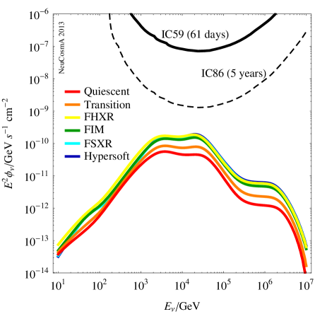
Figure 2: Predictions for the six different X-ray flux states identified by Koljonen et al. (2010), see the legend inside figure. The calculations were done analogous to the hypersoft state for Fig. 1, with a fixed collision radius $l=10^{8}\,\mathrm{c}\mathrm{m}$. As can be seen the variation between the highest predicted flux (for the hypersoft state) and the lowest predicted flux (for the quiescent state) is only of the order of two. Together with the differences in the predicted flux shape this gives a variation of more than three in the expected amount of neutrinos.

We now want to test how many neutrinos would be expected if the observed $\gamma$-ray emission by AGILE was actually coming from the decay of photohadronically produced $\pi^{0}$ into photons. The photons from such decays would have to cascade down to lower energies and may lose a part of their energy during this process. However, here we only want to estimate the number of expected neutrinos for the case that the observed $\mathrm{G}\mathrm{eV}$ emission is due to $\pi^{0}$ decays. Hence, it is sufficient to assume energy conservation for the calculation. With this approach it is possible to set a lower bound on the expected amount of neutrinos. In case of energy losses during/after the cascading process an even higher amount of original $\pi^{0}$ (and consequently $\pi^{+}$) would be needed, and hence an even higher neutrino flux would be expected. If one assumes that

$$\int\limits^{10\,\mathrm{G}\mathrm{eV}}_{10\,\mathrm{M}\mathrm{eV}}\mathrm{d}E_{\gamma}\,E_{\gamma}\frac{\mathrm{d}N_{\gamma}(E_{\gamma})}{\mathrm{d}E_{\gamma}}=\int\limits^{10^{10}\,\mathrm{G}\mathrm{eV}}_{0\,\mathrm{G}\mathrm{eV}}\mathrm{d}E_{\gamma}\,E_{\gamma}\frac{\mathrm{d}N^{\text{HE}}_{\gamma}(E_{\gamma})}{\mathrm{d}E_{\gamma}}$$ (8)

with $\mathrm{d}N_{\gamma}(E_{\gamma})/\mathrm{d}E_{\gamma}$ being the observed photon spectrum from Bulgarelli, A. et al. (2012) while $\mathrm{d}N^{\text{HE}}_{\gamma}(E_{\gamma})/\mathrm{d}E_{\gamma}$ is the resulting spectrum of high-energy photons before cascading to lower energies. The high-energy spectrum has been calculated numerically with the photohadronic interaction code, which also has been used for calculating the neutrino spectra. With this method we obtain that the amount of produced $\pi^{0}$ needed to match the observed $\gamma$-ray emission is about $2400$ times larger than our prediction for $\pi^{0}$ from the calculation for the hypersoft state in the previous section. As a consequence, the nominal amount of expected neutrino events would reach about $5.2$ events for the 61 days of flaring in 2009. Note that such a high amount of events would also be expected for the other flux states. Using the results of the other flux states and normalizing their respective results individually to the AGILE data, we obtain expected amounts of $5.1$–$6.9$ neutrino events under the premise that the observed gamma rays are from $\pi^{0}$ decays. Here, the variation in the result is due to the different flux shapes and not the level of the actual observed photon data, as opposed to the flux predictions in Fig. 2. Nonetheless, these few events would still need to be distinguished from the $\mathcal{O}(100)$ background events. If the used cuts achieve such a high precision, then it should be possible to rule out if the observed flares are due to the decay of $\pi^{0}$.

5 Discussion

In this paper, we have investigated the possibility that MQs may be the sources of high-energy neutrinos. In particular, we have estimated the neutrino flux expected from Cygnus X-3. Starting from the X-ray data for the hypersoft state from Koljonen et al. (2010), we have calculated back to the particle densities of protons and photons inside the jet of Cyg X-3 in the assumption of a simple geometrical model for the jet. The reason for choosing this data set was to use a data for a phase before a radio flare, as suggested by Bulgarelli, A. et al. (2012). This state also fulfills the observed correlation of AGILE $\gamma$-ray flares in 2009 June–July and 2009 November–2010 July with soft X-ray states and episodes of decreasing or non-detectable hard X-ray emission reported by Bulgarelli, A. et al. (2012). However, in principle any other state could also be used for the calculations, as long as we are able to derive the particle densities inside the jet. We then used the densities to compute the expected neutrino emission from the jet using a numerical code which incorporates the full photohadronic interaction cross section, individual treatment of secondary particles (including losses), and flavor mixing of the neutrinos. The expected muon neutrino flux was then compared to the sensitivity of IceCube (59 strings) during the 61 days of flaring. The expected number of $0.02$ events is in concordance with the non-detection of any neutrinos from Cyg X-3 during that period. Assuming an (optimistic) extended period of flaring and a full IC86 detector we expect about $0.84$ associated neutrino events in 5 yr of data taking. Moreover, the shape of the neutrino flux disfavors a detection at $\mathrm{P}\mathrm{eV}$ before seeing events at about $10\,\mathrm{T}\mathrm{eV}$. Additionally, we compared the predicted neutrino flux levels for the flares to the other states identified by Koljonen et al. (2010) to incorporate the dynamic of the source. The resulting change in neutrino flux levels was only of $\mathcal{O}(1)$ and only reduces the expected amount of neutrinos mildly. Nevertheless, these predictions are still subject to some uncertainties due to the not directly measured emission radius as well as the used extrapolated effective area of IceCube. Therefore, even slightly lower amounts of observed neutrinos may not directly contradict the basic model of MQs accelerating protons. Still, in the best case it should be possible to see some events from Cyg X-3 with several years of data taking with the full IceCube detector. Moreover, we also tested the hypothesis that the observed $\gamma$-ray emission is due to the decay of $\pi^{0}$ from photohadronic interactions into photons. We would like to add that the $\pi^{0}$ production of the gamma-ray flux is not likely if “the simplified jet model” is the way gamma rays are produced. In any case to test this hypothesis we compared the integrated energies in the observed photons detected by AGILE to the energy in photons from $\pi^{0}$ decay. In the $\Delta$-resonance approximation, the production of $\pi^{0}$ is directly connected to the production of $\pi^{+}$, and this concept in principle does not change even for a more detailed particle physics treatment of the interactions. Using these calculations, we obtained that the amount of energy in $\pi^{0}$ needed to explain the AGILE observations would have been so high that the number of expected neutrino events would reach about five events during the 61 days of flaring. There have, however, been no reported neutrino events in IceCube which could be associated with Cyg X-3 so far, see Abbasi et al. (2013). We can therefore start to rule out that the observed $\gamma$-ray emission is due to the decay of $\pi^{0}$ from photohadronic interactions by combining the photon and neutrino data in the coming months. Especially, the point source analysis of IC59 would be of great interest in this regard.

References

- Abbasi et al. (2011) Abbasi, R., et al. 2011, Astrophys.J., 732, 18
- Abbasi et al. (2013) —. 2013, Astrophys.J., 763, 33
- Ahn et al. (2012) Ahn, J., et al. 2012, Phys.Rev.Lett., 108, 191802
- Ahrens et al. (2003) Ahrens, J., et al. 2003, Nucl. Phys. Proc. Suppl., 118, 388
- An et al. (2012) An, F., et al. 2012, Phys.Rev.Lett., 108, 171803
- Baerwald et al. (2011) Baerwald, P., Hümmer, S., & Winter, W. 2011, Phys. Rev., D83, 067303
- Bulgarelli, A. et al. (2012) Bulgarelli, A., Tavani, M., Chen, A. W., et al. 2012, A&A, 538, A63
- Distefano et al. (2002) Distefano, C., Guetta, D., Waxman, E., & Levinson, A. 2002, Astrophys.J., 575, 378
- Dubus et al. (2010) Dubus, G., Cerutti, B., & Henri, G. 2010, MNRAS, 404, L55
- Fender (2001) Fender, R. 2001, in American Institute of Physics Conference Series, Vol. 558, American Institute of Physics Conference Series, ed. F. A. Aharonian & H. J. Völk, 221–233
- Fermi LAT Collaboration et al. (2009) Fermi LAT Collaboration, Abdo, A. A., Ackermann, M., et al. 2009, Science, 326, 1512
- Hümmer et al. (2010a) Hümmer, S., Maltoni, M., Winter, W., & Yaguna, C. 2010a, Astropart. Phys., 34, 205
- Hümmer et al. (2010b) Hümmer, S., Rüger, M., Spanier, F., & Winter, W. 2010b, Astrophys. J., 721, 630
- Ishihara (2013) Ishihara, A. 2013, Nuclear Physics B - Proceedings Supplements, 235 - 236, 352 , the XXV. International Conference on Neutrino Physics and Astrophysics
- Koljonen et al. (2010) Koljonen, K. I. I., Hannikainen, D. C., McCollough, M. L., Pooley, G. G., & Trushkin, S. A. 2010, MNRAS, 406, 307
- Levinson & Waxman (2001) Levinson, A., & Waxman, E. 2001, Phys.Rev.Lett., 87, 171101
- Ling et al. (2009) Ling, Z., Zhang, S. N., & Tang, S. 2009, Astrophys.J., 695, 1111
- Mioduszewski et al. (2001) Mioduszewski, A. J., Rupen, M. P., Hjellming, R. M., Pooley, G. G., & Waltman, E. B. 2001, Astrophys.J., 553, 766
- Mirabel & Rodriguez (1999) Mirabel, I., & Rodriguez, L. 1999, Ann.Rev.Astron.Astrophys., 37, 409
- Mücke et al. (2000) Mücke, A., Engel, R., Rachen, J., Protheroe, R., & Stanev, T. 2000, Comput.Phys.Commun., 124, 290
- Piano et al. (2012) Piano, G., et al. 2012, Astron.Astrophys., 545, A110
- Reynoso & Romero (2009) Reynoso, M. M., & Romero, G. E. 2009, Astron. Astrophys., 493, 1
- Romero et al. (2003) Romero, G. E., Torres, D. F., Bernado, M. K., & Mirabel, I. 2003, Astron.Astrophys., 410, L1
- Tavani et al. (2009) Tavani, M., Bulgarelli, A., Piano, G., et al. 2009, Nature, 462, 620
- Torres & Reimer (2011) Torres, D. F., & Reimer, A. 2011, A&A, 528, L2