The debris disk around $\gamma$ Doradus resolved with Herschel

Abstract

We present observations of the debris disk around $\gamma$ Doradus, an F1V star, from the Herschel Key Programme DEBRIS (Disc Emission via Bias-free Reconnaissance in the Infrared/Submillimetre). The disk is well-resolved at 70, 100 and 160 µm, resolved along its major axis at 250 µm, detected but not resolved at 350 µm, and confused with a background source at 500 µm. It is one of our best resolved targets and we find it to have a radially broad dust distribution. The modeling of the resolved images cannot distinguish between two configurations: an arrangement of a warm inner ring at several AU (best-fit 4 AU) and a cool outer belt extending from $\sim$55 to 400 AU or an arrangement of two cool, narrow rings at $\sim$70 AU and $\sim$190 AU. This suggests that any configuration between these two is also possible. Both models have a total fractional luminosity of $\sim$$10^{-5}$ and are consistent with the disk being aligned with the stellar equator. The inner edge of either possible configuration suggests that the most likely region to find planets in this system would be within $\sim$55 AU of the star. A transient event is not needed to explain the warm dust’s fractional luminosity.

1. Introduction

Debris disks were first discovered when observations with the InfraRed Astronomical Satellite (IRAS) revealed that Vega, $\beta$ Pictoris, and Fomalhaut were unexpectedly bright at infrared (IR) wavelengths (Aumann et al. 1984). Many main-sequence stars have since been observed to possess IR emission above the expected photospheric level, which is usually attributed to the thermal emission of dust that is heated by the host star(s). The dust is second generation, e.g., produced by ongoing collisions of larger bodies, since the dust’s lifetime in orbit is too short for it to be primordial in origin, e.g., originating in the protoplanetary disk (Backman & Paresce 1993). Models suggest that parent planetesimals of at least 10–100 km feed the dust through destructive collisions, though how objects are initially “stirred” to high enough collision velocities is unclear (e.g., Wyatt et al. 2007). One possibility is the formation of bodies large enough ($>$1000km) to stir planetesimals through dynamical interactions (Kenyon & Bromley 2004; Mustill & Wyatt 2009).

Modelling of the stellar spectral energy distribution (SED) at optical wavelengths allows a comparison with the observed IR flux, and possible detection of an IR excess. Modelling the SED of the excess itself provides a measure of the dust temperature and therefore its location (by making assumptions about the emissive properties of the dust). This method has proven instrumental in relating the properties of debris disks to each other. It is generally sufficient to assume that the dust particles behave like blackbodies, but this approach does not yield the exact disk location because dust at different stellocentric distances can have the same temperature (grain size and dust location are degenerate). SED modeling can also yield incorrect dust properties such as lower grain size (compare HD107146, Roccatagliata et al. 2009 versus Ardila et al. 2004 and Ertel et al. 2011).

Thus resolving a disk allows for a deeper understanding of the system since its configuration is directly observed. Disk sizes determined from resolved images are often found to be $\sim$2–5 times larger than those suggested by the SED with blackbody assumptions (Schneider et al. 2006; Wyatt 2008; Matthews et al. 2010; Rodriguez & Zuckerman 2012; Booth et al., in press). Resolving the disk at more than one wavelength is even more advantageous, as it can reveal whether the observed configuration of the system is wavelength dependent, as it is for Vega (Su et al. 2005; Sibthorpe et al. 2010), $\beta$ Leo (Matthews et al. 2010; Churcher et al. 2011) and others. For example, a disk may appear larger at longer wavelengths if it has two components, and the cooler one (i.e., further from the star) dominates at the longer wavelength, as is the case for $\eta$ Corvi (Wyatt et al. 2005; Matthews et al. 2010).

As more data are collected on debris disks from observatories with improved sensitivity and resolution, we are moving away from the simple disk models of single narrow dust rings and discovering more complicated shapes and configurations. Many debris disks have been found to contain multiple dust components and/or have extended dust distributions with a large range in behaviour (e.g., HD 107146: Ertel et al. 2011, $\beta$ Leo: Stock et al. 2010, $\zeta$ Lep: Moerchen et al. 2007). Some hosts that have multi-component disks are also planet hosts (e.g., $\epsilon$ Eridani: Backman et al. 2009; Reidemeister et al. 2011). HR 8799 even plausibly shows the existence of a planetary system with warm and cold dust that has planets in the gap (Su et al. 2009). This highlights the rich diversity of observed planetary systems.

Since debris disks were discovered with IRAS, significant advancement of the field has been made with other observatories such as the Spitzer Space Telescope (Spitzer; (Rieke et al. 2005; Beichman et al. 2006; Bryden et al. 2009), the James Clerk Maxwell Telescope (Holland et al. 1998; Greaves et al. 1998), and now the Herschel Space Observatory (Herschel) by observing the thermal emission of the dust. (Optical observations of star light scattered by dust are also used to study debris disks.) Herschel is well suited for debris disk studies as dust emission is well contrasted against stellar emission at its wavelength range of 70–500 µm. It is sensitive enough to detect the photospheres of nearby stars (and therefore can better determine whether an excess is present), and its resolution of 6.7″ at 100 µm can probe the sizes of nearby disks. We present observations of $\gamma$ Doradus ($\gamma$ Dor) and its debris disk that were taken with Herschel as part of the DEBRIS (Disc Emission via Bias-free Reconnaissance in the Infrared/Submillimetre) Key Programme (Matthews et al. 2010). Stars observed by DEBRIS are taken from the UNS (Unbiased Nearby Stars) sample (Phillips et al. 2010), a volume-limited sample, and so unbiased toward spectral type, binarity, metallicity, and presence of known planets.

Table 1Stellar Information for $\gamma$ Dor

Parameter		Value		Reference
Spectral type		F1 V		Gray et al. (2006)
R.A. (J2000)		04:16:01.586		Høg et al. (2000)
Decl. (J2000)		–51:29:11.933		Høg et al. (2000)
PM-R.A. (mas yr-1)		101.5		Høg et al. (2000)
PM-decl. (mas yr-1)		184.7		Høg et al. (2000)
$V$ magnitude		4.25		Balona et al. (1994)
Distance (pc)		20.46 $\pm$ 0.15		Phillips et al. (2010)
Age (Gyr)		0.4		Chen et al. (2006)
Age (Gyr)		0.82–2.19		Vican (2012)

The debris disk around $\gamma$ Dor (HD 27290, HIP 19893), whose basic parameters are listed in Table 1, was discovered with IRAS (Aumann 1985; Rhee et al. 2007). It has been detected with Spitzer but was not resolved (Chen et al. 2006; Koerner et al. 2010). Here we present images of the $\gamma$ Dor disk taken with Herschel that are the first to directly constrain the location of the dust. $\gamma$ Dor is not known to host any extra-solar planets but is a target for the exoplanet search using Near-Infrared Coronagraphic Imager (NICI) on the Gemini-South 8.1 m telescope (Chun et al. 2008; Liu et al. 2010), the results of which are not yet publicly available. In Section 2, we present the Herschel observations and ancillary data. We measure the Herschel fluxes in Section 3. In Section 4, $\gamma$ Dor’s photosphere is modeled and used to determine the excesses that are observed in the IR and submillimetre (submm). We present a basic analysis of the images in Section 5 and the more detailed modeling of the SED and resolved images in Section 6. The results are discussed in Section 7 and we summarize our conclusions in Section 8.

2. Herschel Observations

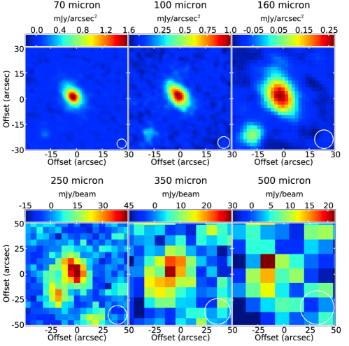
Figure 1.— PACS (top row) and SPIRE (bottom row) Herschel observations showing the 60″ $\times$ 60″ and 100″ $\times$ 100″ regions around $\gamma$ Dor, respectively. The beam sizes (the FWHMs of the PSFs) are shown in the bottom right corners. A point-like background source is evident $\sim$30″ to the southeast of $\gamma$ Dor (up is North). The extended emission from $\gamma$ Dor is evident in comparison to the background source and the beam sizes. The background source is well separated from $\gamma$ Dor at PACS wavelengths, but becomes increasingly difficult to distinguish from $\gamma$ Dor at SPIRE wavelengths. At 500 µm, the flux from both sources is contained within a single beam.

Table 2Herschel Observations

ObsID	Instrument	Band	Time on Target	Scan Rate	Date(s)	Beam Size	Noise
		(µm)	(s)	(″ s-1)	Observed	(″)	(mJy)
1342193149/50	PACS	100	1129	20	2010 Mar 31	6.69 $\times$ 6.89	1.3
1342193149/50	PACS	160	1129	20	2010 Mar 31	10.65 $\times$ 12.13	3.4
1342220766/67	PACS	70	1129	20	2011 Apr 29	5.46 $\times$ 5.76	1.2
1342220766/67	PACS	160	1129	20	2011 Apr 29	10.65 $\times$ 12.13	2.7
1342204956	SPIRE	250	901	30	2010 Sep 21	18.7 $\times$ 17.5	4.9
1342204956	SPIRE	350	901	30	2010 Sep 21	25.6 $\times$ 24.2	7.3
1342204956	SPIRE	500	901	30	2010 Sep 21	38.2 $\times$ 34.6	5.3

Note. — Beam sizes from PACS Observer’s Manual v2.3 and SPIRE Observer’s Manual v2.4.

Broadband photometric mapping observations were performed at 70, 100, 160, 250, 350, and 500 $\mu$m using the Photoconductor Array Camera and Spectrometer (PACS; Poglitsch et al. 2010) and Spectral and Photometric Imaging Receiver (SPIRE; Griffin et al. 2010) instruments on board Herschel (Pilbratt et al. 2010). These observations were performed as part of the DEBRIS key programme (B. C. Matthews et al., in preparation) and were performed in mini and small scan-map modes for PACS and SPIRE, respectively. PACS observes at 100 and 160 µm simultaneously or at 70 and 160 µm simultaneously. Since $\gamma$ Dor was observed at both 70 and 100 µm, $\gamma$ Dor was observed at 160 µm twice and the map at this wavelength is composed of the data from both observations. The coordinates of the peak of the emission in the 70 and 100 µm maps are used to align 160 µm maps. A summary of the observation parameters is given in Table 2.

The PACS data were reduced using HIPE (Herschel Interactive Processing Environment: Ott 2010) version 7.0 Build 1931. The reduction method includes some data that were taken while the telescope was reversing the scan direction, and therefore not scanning at a constant speed, to decrease the noise in the map. This reduces the noise at the map centre (where the target is located) by $\sim$25%. PACS data are subject to 1/f noise, whose power spectrum is a function of the noise at a given angular scale (determined by the scan rate of the telescope). To maximize the signal-to-noise in our maps, we filter out signals on angular scales larger than 66, 66, and 100″ at 70, 100, and 160 µm in the map generation process. The SPIRE data were also reduced using the standard Herschel pipeline script in HIPE.

Figure 1 shows the 60″ $\times$ 60″ region around $\gamma$ Dor at 70, 100, and 160 µm and the 100″ $\times$ 100″ region at 250, 350, and 500 µm. A background source, which is not listed in the NASA/IPAC Extragalactic Database (NED) or the NASA/IPAC Infrared Science Archive, is visible $\sim$30″ to the southeast. The emission from $\gamma$ Dor and its disk is well resolved with PACS at 70, 100, 160 µm and marginally resolved at 250 µm. The respective full width half maxima (FWHMs) of the star+disk observations at 70, 100, 160, 250 and 350 µm are 10.2″ $\times$ 7.3″, 12.7″ $\times$ 7.9″, 19.2″ $\times$ 13.1″, 26.0″ $\times$ 19.1″ and 27.5″ $\times$ 22.8″ compared to the FWHMs for a standard star of 5.6″, 6.8″, 11.4″, 18.2″and 24.9″ (these are the geometric means of the beam sizes listed in Table 2). Emission is detected at all Herschel wavelengths, however, the background source to the southeast, which is well separated from the disk at 70–160 µm, is harder to separate at SPIRE wavelengths. At 250 and 350 µm, the nearby background source and $\gamma$ Dor begin to blend together, whereas at 500 µm, the two are indistinguishable.

3. Herschel flux measurements

Two methods are used to measure fluxes in the Herschel maps: aperture photometry is used when the emission is resolved and a point-spread function (PSF) is fit to the source when it is unresolved. Thus the flux from $\gamma$ Dor is measured with aperture photometry at 70–250 µm, and PSF fitting at 350 and 500 µm. The southeast background source is consistent with a point source in the maps, and so it is fit with a PSF at all wavelengths. The PSF fit is done after rotating the instrumental PSF to match the rotation of the telescope at the time of the observations and using a $\chi^{2}$ minimization method. Herschel observations of the diskless star $\alpha$ Boo are reduced in the same manner as the DEBRIS data and used as the instrumental PSF at PACS wavelengths. Empirical SPIRE PSFs are downloaded from the ESA ftp site.

Table 3 Observed Fluxes and Predicted Photospheric Fluxes

Wavelength	Observed Flux	Instrument	Method	Photosphere	Excess	Reference
(µm)	(Jy)	or Satellite		(Jy)	(mJy)
0.4	59.8 $\pm$ 0.8	Hipparcos	$\cdots$	59.7 $\pm$ 1.1	$\cdots$	Høg et al. (2000)
0.5	74.4 $\pm$ 0.8	Hipparcos	$\cdots$	74.8 $\pm$ 1.4	$\cdots$	Høg et al. (2000)
0.6	71.5 $\pm$ 1.4	Hipparcos	$\cdots$	71.7 $\pm$ 1.3	$\cdots$	Perryman & ESA (1997)
0.5	76.5 $\pm$ 1.5	Hipparcos	$\cdots$	75.7 $\pm$ 1.4	$\cdots$	Mermilliod (2006)
1.2	53.7 $\pm$ 12.0	2MASS	$\cdots$	55.2 $\pm$ 1.0	$\cdots$	Cutri et al. (2003)
9.0	1.908 $\pm$ 0.035	AKARI	$\cdots$	1.924 $\pm$ 0.035	$\cdots$	Ishihara et al. (2010)
12.0	1.202 $\pm$ 0.051	IRAS	$\cdots$	1.179 $\pm$ 0.022	$\cdots$	Moshir et al. (1990)
	(mJy)			(mJy)
18.0	514.2 $\pm$ 21.0	AKARI	$\cdots$	494.1 $\pm$ 9.1	$\cdots$	Ishihara et al. (2010)
23.7	315.6 $\pm$ 3.2	MIPS	PSF fit	286.0 $\pm$ 5.3	29.6 $\pm$ 6.2	K. Su, private communication
25.0	292.3 $\pm$ 22.0	IRAS	$\cdots$	256.7 $\pm$ 4.7	$\cdots$	Moshir et al. (1990)
60.0	196.7 $\pm$ 11.0	IRAS	$\cdots$	44.2 $\pm$ 0.8	$\cdots$	Moshir et al. (1990)
71.4	170.7 $\pm$ 8.1	MIPS	PSF fit	31.1 $\pm$ 0.6	139.6 $\pm$ 8.1	K. Su, private communication
70.0	171.0 $\pm$ 8.7	PACS	30 $\times$ 19″ aperture	31.1 $\pm$ 0.6	139.5 $\pm$ 8.8	This work
100.0	$<$476.7	IRAS	$\cdots$	15.7 $\pm$ 0.3	$\cdots$	Moshir et al. (1990)
100.0	148.4 $\pm$ 7.7	PACS	30 $\times$ 17″ aperture	15.7 $\pm$ 0.3	132.7 $\pm$ 7.8	This work
160.0	134.3 $\pm$ 14.1	PACS	30 $\times$ 20″ aperture	6.4 $\pm$ 0.1	127.9 $\pm$ 14.1	This work
250.0	52.5 $\pm$ 6.5	SPIRE	30 $\times$ 24″ aperture	2.45 $\pm$ 0.05	50.0 $\pm$ 6.5	This work
350.0	23.5 $\pm$ 8.0	SPIRE	PSF fit	1.24 $\pm$ 0.02	22.2 $\pm$ 8.0	This work
500.0	$<$16.7 $\pm$ 5.9	SPIRE	PSF fit	0.60 $\pm$ 0.01	$<$16.1 $\pm$ 5.9	This work

At 250 and 350 µm, where the background source is not well separated from the $\gamma$ Dor disk, two PSFs are fit simultaneously to the expected positions of each source. As a result, the disk flux at 350 µm is very uncertain (as well as the background source flux at 250 and 350 µm). We quote the flux at 500 µm from a single PSF fit as an upper limit since the background source and the disk are within the same beam. The coordinates of the background source are determined from the 160 µm map, where it is both bright and well separated from the $\gamma$ Dor emission. The position of the PSF fit to $\gamma$ Dor is fixed to its expected coordinates at the time of the observations, given its proper motion (Table 1). This is reasonable as there is no evidence of an offset between the disk centre and the stellar position given that the location of the emission is 1.4 and 2.7″ from $\gamma$ Dor’s expected position at 70 and 100 µm (determined from the PSF fit) and therefore within Herschel’s 2.3″ pointing uncertainty (Herschel Observers’ Manual v4).

The uncertainty in the flux is determined from the noise, listed in Table 2, measured by fitting a PSF to 400 random locations (the flux is the only free parameter) within a region devoid of significant emission and of similar coverage as the map centre (see B. C. Matthews et al., in preparation). (This is scaled by the area of the aperture for aperture-measured fluxes.) The PACS calibration accuracies of 3%, 3%, and 5% at 70, 100, and 160 µm, respectively (PACS Observer’s Manual v2.3), and SPIRE pixel size correction factors and absolute flux calibration accuracy of 7% (SPIRE Observer’s Manual v2.4) are added in quadrature. The measured fluxes of $\gamma$ Dor are listed in Table 3. The fluxes of the southeast background source are 11.4 $\pm$ 1.7, 20.0 $\pm$ 1.9, 35.0 $\pm$ 4.6, 28.0 $\pm$ 5.7, 18.5 $\pm$ 7.9, and $<$16.7 $\pm$ 5.9 mJy at 70, 100, 160, 250, 350, and 500 µm. The 350 µm detection is only a 2.5$\sigma$ detection and the 500 µm 3$\sigma$ detection (with respect to the map noise in Table 2) includes both $\gamma$ Dor and the background source.

Filtering out signals on large angular scales is necessary to reduce the noise (see Section 2 for more details), however, it also filters out the large angular scales of the PACS beam, which extends to about 17 arcmin. As a result, the fluxes measured in the PACS maps are too low. We correct for this by scaling our fluxes by 1.16 $\pm$ 0.05, 1.19 $\pm$ 0.05, and 1.21 $\pm$ 0.05 at 70, 100, and 160 µm (Kennedy et al. 2012). These correction factors are determined by comparing the fluxes of bright point sources in DEBRIS maps to their predicted photospheric flux. It should be noted that these correction factors are determined for point sources, but they are reasonable to use for an extended source, such as $\gamma$ Dor, since the angular scales of the filtering are still large in comparison to the angular scale of $\gamma$ Dor’s emission.

4. Photosphere and Excesses

4.1. Modelling the Stellar Photosphere

Accurate models of the stellar photosphere are crucial for debris disk studies, as the analysis is based on emission that is observed in excess of expected photospheric emission. The stellar photosphere is modeled using a $\chi^{2}$ minimization method to fit stellar models from the Gaia grid (Brott & Hauschildt 2005) to the observed optical and near-IR fluxes (see Table 3). The modeling of the stellar photosphere is done consistently for all DEBRIS targets (see Kennedy et al. 2012 for more details).

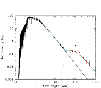
Figure 2.— SED for $\gamma$ Dor. Herschel fluxes are shown in red. The IRS spectrum is plotted in blue. Fluxes which contain a contribution from a background source (IRAS fluxes and our 500 µm flux) are displayed with open circles. Upper limits are shown with triangles. The black line traces the photospheric model (Section 4.1). The green dotted line traces a sample 70 K blackbody spectrum to compare to the shape of the excess spectrum. The solid green line traces the total flux from $\gamma$ Dor and the sample blackbody.

A photospheric model with a $T_{\rm{eff}}$ of 7204 $\pm$ 28 K, a $\log(g)$ of 3.49 $\pm$ 0.1, an $[\rm{M/H}]$ of $-0.41$ $\pm$ 0.17, an $R_{*}$ of 1.67 $\pm$ 0.22 R_⊙ and an $L_{*}$ of 6.7 $\pm$ 0.1 L_⊙ is used. Given the uncertainties in deriving $\log(g)$ and [M/H] from SED modeling, the results are in good agreement (within 0.1 dex and 0.3 dex, respectively) of Gray et al. (2006). The predicted photospheric fluxes from the stellar fit are compared to the observed fluxes and used to measure the excess emission in Table 3. The SED is shown in Figure 2 with the photospheric model.

4.2. Spitzer Excesses

We include Spitzer Infrared Spectrograph (IRS) observations of $\gamma$ Dor downloaded from the Cornell Atlas of Spitzer/IRS Sources (CASSIS). This spectrum is from Ardila et al. (2010) and includes AOR 24368640, AOR 27577600, and AOR 3555584. It is consistent with no excess shortward of 22 µm and is therefore in agreement with AKARI fluxes that measure no excesses shortward of 18 µm.

5. Basic image analysis

Table 4 2D Gaussian Disk Fits

Band	Beam	$\theta_{\rm{obs,maj}}$	$\theta_{\rm{obs,min}}$	$\theta_{\rm{act,maj}}$	$\theta_{\rm{act,min}}$	Inclination	Position Angle
(µm)	(″)	(″)	(″)	(″)	(″)	(∘)	(∘)
70	5.61	12.7 $\pm$ 0.7	7.9 $\pm$ 0.4	11.4 $\pm$ 0.8	5.6 $\pm$ 0.6	61 $\pm$ 6	56 $\pm$ 6
100	6.79	14.2 $\pm$ 0.7	8.2 $\pm$ 0.4	12.5 $\pm$ 0.8	4.6 $\pm$ 0.7	68 $\pm$ 5	52 $\pm$ 4
160	11.36	20.2 $\pm$ 0.8	13.3 $\pm$ 0.5	16.6 $\pm$ 1.0	6.9 $\pm$ 1.0	65 $\pm$ 5	62 $\pm$ 5
250	18.2	26.3 $\pm$ 4.2	19.3 $\pm$ 3.1	19.0 $\pm$ 5.8	$\cdots$	$>$52	55 $\pm$ 22
350	24.9	26.3 $\pm$ 6.9	22.7 $\pm$ 6.8	$\cdots$	$\cdots$	$\cdots$	$\cdots$

The size of the disk can be estimated by fitting 2D Gaussians to the images. First, a model of the photosphere is removed from the image by subtracting a PSF that is scaled to the expected photospheric emission (Section 4.1). The FWHMs and position angles of the 2D Gaussian models are listed in Table 4. The quoted error on a fitted parameter gives the range of parameter values for which the $\chi^{2}$ value is within 10% of the minimum $\chi^{2}$ value. The $\chi^{2}$ value is measured in a small region around $\gamma$ Dor.

The major and minor FWHMs are deconvolved from the beam size using

$$\theta_{\rm{obs}}^{2}=\theta_{\rm{act}}^{2}+\theta_{\rm{beam}}^{2},$$ (1)

where $\theta_{\rm{act}}$ is the actual angular size of the object, $\theta_{\rm{beam}}$ is the effective beam size and $\theta_{\rm{obs}}$ is the observed angular size of the object. (This is the relation for convolving a Gaussian with a Gaussian.) Assuming the true shape of the disk is azimuthally symmetric, the deconvolved major and minor FWHMs are used to estimate an inclination of $\sim$65^∘ from a face-on orientation (see Table 4) that is consistent with the more detailed image modeling (see Section 6.3).

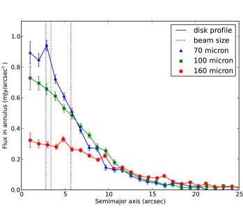
Figure 3.— Surface brightness profiles of the $\gamma$ Dor disk. The average surface brightness in elliptical annuli with increasing semi-major axis at 70 (blue triangles), 100 (green squares) and 160 (red circles) µm. 1$\sigma$ errors are shown. The stellar model is subtracted from the maps to measure the profile of the disk (solid lines). (The model of the nearby background source is also subtracted from the maps.) Beam sizes (dotted lines) are plotted for comparison. The shape of the profile is consistent with a radial distribution of dust where the cooler dust is brighter and the warmer dust is fainter at longer wavelengths (see the text). The surface brightness profiles fall off to similar levels beyond $\sim$10″ at all wavelengths.

The fitted parameters of the 2D Gaussian models are used to define elliptical annuli to measure the surface brightness profiles of the disk in the 70, 100, and 160 µm images where the disk is resolved along both the major and minor axes. Figure 3 shows that the shape of the profiles is wavelength dependent. This is consistent with a broad radial distribution of material as dust further from the star will be cooler and dominate the flux at longer wavelengths. This is also reflected in the larger FWHMs at longer wavelengths listed in Table 4. The underlying dust distribution is investigated by modeling the images in the following section.

6. Disk modeling

6.1. Basic Model

We first present the underlying set up of the debris disk modeling that we implement in Sections 6.2 and 6.3, to introduce the various parameters. The simple approach to modeling debris disks is to assume that the dust is contained within a narrow/discrete ring at some distance from the host star. This model is easily extended to model multiple narrow/discrete rings by summing up the individual contributions of each ring using a modified blackbody function (Dent et al. 2000),

$$F_{\nu}=2.35\times 10^{-11}~{}d^{-2}~{}\sum_{R}~{}\sigma(R)~{}B_{\nu}(\lambda,T(R))~{}X_{\lambda}^{-1}$$ (2)

where $F_{\nu}$ is the flux density (in Jy) at wavelength $\lambda$ (in µm), $d$ is the distance to the star (in pc), and $\sigma(R)$ is the cross-sectional area (in AU²) of the ring at radius $R$ (in AU). $B_{\nu}(\lambda,T(R))$ is the Planck function (in Jy sr^-1) for the ring at radius R with temperature T (in K). Equation (2) is modified by $X_{\lambda}$, where $X_{\lambda}=(\lambda/\lambda_{0})^{\beta}$ for wavelengths longer than $\lambda_{0}$ and $X_{\lambda}=1$ otherwise. This accounts for the fall off of the spectrum that is observed to be steeper than the blackbody function at submm wavelengths for most debris disks (Dent et al. 2000).

If the dust grains act like blackbodies, the radius of a dust ring can be derived from its temperature given the luminosity of the star, $L_{*}$:

$${R_{bb}}=278.3^{2}~{}L_{*}^{1/2}~{}T^{-2}.$$ (3)

However, using the above method to model the SEDs of debris disks typically underestimates the observed sizes of the disks by a factor of 2–5 (Schneider et al. 2006; Wyatt 2008; Matthews et al. 2010; Rodriguez & Zuckerman 2012; Booth et al., accepted, and references therein) because grains with a lower radiation efficiency, dependent on their size and composition, will be hotter than blackbody grains at the same distance would.

Equation (2) can be expanded to model dust in a wide/extended belt by treating the belt as a series of dust rings and setting $\sigma$ and $T$ to follow power-law distributions. The cross-sectional area is determined from the optical depth, $\tau(R)$, given by

$$\tau(R)=\tau_{0}~{}(R/R_{0})^{-\gamma},$$ (4)

where $\tau_{0}$ is the optical depth at $R_{0}=1$ AU and $\gamma$ describes the fall off of the surface density at further distances from the star. Similarly, $T(R)$ is given by,

$$T(R)=T_{0}~{}(R/R_{0})^{-\delta},$$ (5)

where $T_{0}$ is the temperature at $R_{0}=1$ AU and $\delta$ describes how quickly the temperature of the dust grains declines at larger radii from the star. The blackbody temperature distribution given in Equation (3) has the values of $\delta=0.5$ and $T_{0}=438.4$ K for $\gamma$ Dor. The cross-sectional area, $\sigma$, the fractional luminosity, $f_{d}$, and the optical depth, $\tau$, of the dust are related by $\sigma(R)~{}=~{}2\pi\,R\,{dR}\,\tau(R)\,=\,f_{d}\,4\pi\,R^{2}$ (see Krivov 2010 for a review). For a narrow/discrete ring model, we assume $dR/R=0.1$.

This construct is valid for modeling both the SED and the resolved images. The SED modeling traces the temperatures of the dust within the disk (e.g., $T$, $\sigma$), whereas the image modeling constrains its physical arrangement ($R$ and therefore the dependence of $T$ and $\sigma$ on $R$). This approach (used for all DEBRIS modeling papers) parameterizes the shape of the SED at each radius. How that shape relates to the physical parameters of dust composition and size distribution will be discussed in a later paper.

6.2. SED Modelling

For the majority of debris disks, only unresolved photometry is available. We include an analysis of the SED without the resolved spatial information to highlight how the resolved images reduce the ambiguities. A single dust temperature is unable to account for the spectral breadth of the excess emission (Figure 2). We therefore model the SED with two different extended temperature distributions: a model of two discrete dust rings and a model of a single extended dust belt. All models have the same fractional luminosity of $2.6\times 10^{-5}$.

The SED model of two discrete rings accounts for the broad shape of the SED with a warm ring ($T$ $\sim$ 125 K, $R_{bb}$ $\sim$ 12 AU) that dominates the flux at IRS wavelengths and a cool ring ($T$ $\sim$ 50 K, $R_{bb}$ $\sim$ 77 AU) that accounts for the Herschel fluxes. This model implies that the Herschel images would be dominated by dust at a single temperature.

The extended belt SED model requires a relatively flat profile of the cross-sectional area ($\gamma\sim 0$ in Equation (4)) to account for the similar fluxes at 70, 100, and 160 µm and the mid-IR (IRS and MIPS 24) excesses. Using a blackbody temperature distribution, this model suggests that the dust extends from $\sim$13 AU to $\sim$166 AU.

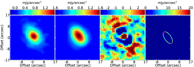
Figure 4.— An attempted single narrow ring model of the $\gamma$ Dor disk. Left to right: the observations, the simulated Herschel observations of the model, the residuals, and simulated observations of the model at high resolution at 70 µm. The color scale of the residuals extends from $-3\sigma$ to 3$\sigma$. Clearly the single narrow ring model cannot adequately explain the observed emission and we must turn to a model that includes dust at a range of radii.

The immediate contrast between unresolved and resolved photometry is evident in the predictions from the SED models. The SED model of two discrete rings suggests that the Herschel fluxes are dominated by a single narrow ring at 77 AU, however, the resolved images show an extended distribution of dust that cannot be modeled with a single ring, as shown in Figure 4. The discrepancies between what would be interpreted from the SED and what is revealed by modeling resolved images (see the following section) are clear. Resolved imaging is the only way to constrain the possible spatial distributions.

Table 5 Fitted Parameters for the Two Narrow Rings
wwhhiitte Model of the Herschel Images

Parameter	Value
$R_{1}$	70 AU
$R_{2}$	190 AU
$\tau_{2-1}$	0.85
Inclination	71∘
Position angle	55.9∘ N of E
70 µm flux	140 mJy
100 µm flux	142 mJy
160 µm flux	125 mJy

6.3. Image Modelling

To keep the results from SED modeling and image modeling distinct, we describe our imaging models as “narrow rings” and “wide belt” which are analogous to the “discrete rings” and “extended belt” SED models, but of course with different fit parameters. We also refer to the dust observable to Herschel as “cool dust” and dust that is responsible for any excesses at shorter wavelengths (IRS and MIPS 24) that does not effect the Herschel observations as “warm dust.”

The extended spatial distribution of dust is clear in the images. The best-fit imaging model of a single narrow dust ring is unable to account for the emission on the largest and smallest scales (see Figure 4). Although the images show that all the dust cannot lie at the same stellocentric radius, the resolution of Herschel is not sufficient to distinguish between different extended configurations. Below, we show that both a model of two narrow rings of dust and a model of a wide belt of dust are able to reproduce the observations of the cool dust component. Both models are parameterized by an inner radius and an outer radius. (A constant opening angle of 10^∘ was used and reasonable variations to this do not affect the fitting.) The narrow rings model describes two discrete dust components at these radii with no dust between them whereas the wide belt model is described by a smooth distribution of material between these edges. We do not intend to fully investigate the possible parameter space given the limited resolution. Rather, we compare the two models to demonstrate the uncertainties on the radial extent of the disk. These two extended spatial distributions are reasonable to consider as they are observed in other resolved debris disks (e.g., $\eta$ Corvi: Wyatt et al. 2005; Matthews et al. 2010, HR 8799: Su et al. 2009, HD 181327: Schneider et al. 2006). The two configurations are modeled with similar techniques at 70, 100, and 160 µm, where the $\gamma$ Dor disk is well separated from the nearby background source. A $\chi^{2}$ grid analysis is used for the two narrow rings model (as in Booth et al., accepted), and a combination of by-hand and $\chi^{2}$ minimization (as in Kennedy et al. 2012 and Wyatt et al. 2012) is used for the wide belt model.

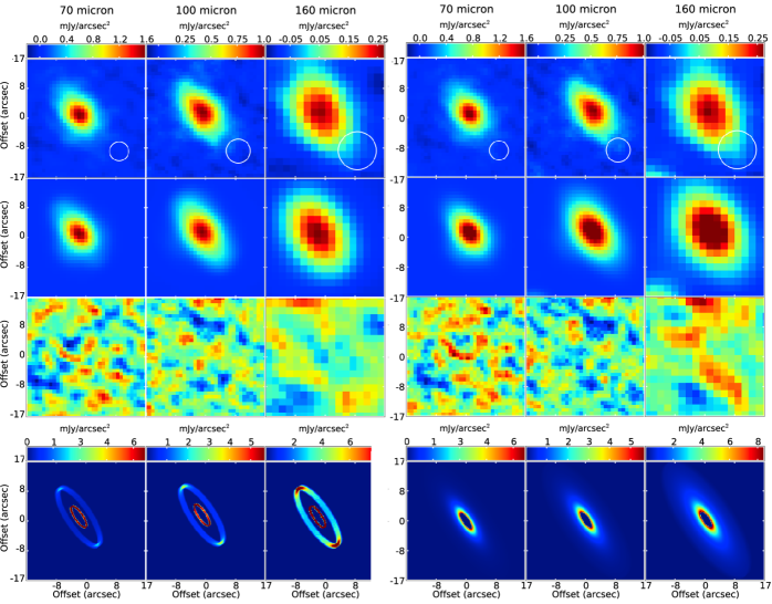
Figure 5.— Imaging models of the $\gamma$ Dor disk. (top to bottom) The observations, the simulated Herschel observations of the model, the residuals, and the simulated observations of the model at high resolution at (left to right) 70, 100 and 160 µm for the imaging models of the cool dust. The narrow rings model is on the left, and the wide belt model is on the right (see the text). The color scale for the residuals map extends from $-3\sigma$ to $+3\sigma$. The residuals show that both models of the cool dust successfully reproduce the resolved PACS observations.

Table 6 Fitted Parameters for the Wide Belt Model
wwhhiitte of the Herschel Images

Parameter	Value
Inner radius	55 AU
Outer radius	400 AU
$\tau_{0}$	$3.4\times 10^{-5}$
$\gamma$	0.8
$T_{0}$	585 K
$\delta$	0.5
Inclination	68.5∘
Position angle	55.6∘ N of E

The best-fit imaging model of two narrow rings is determined using a grid of parameters: the radius of the inner ring ($R_{1}$), the radius of the outer ring ($R_{2}$), the inclination of the disk, and the ratio of the optical depths of the two rings ($\tau_{2-1}=\tau_{1}/\tau_{2}$, where $\tau_{1}$ and $\tau_{2}$ are the $\tau$ for the inner and outer rings, respectively). The grid size (and therefore computation time) is minimized by fixing the position angle of the disk to that determined from the 2D Gaussian model of the 70 µm image (Section 4). Additionally, for each set of grid parameters, the total disk flux, and therefore the total $\tau$ of the system, is fit using the package MPFIT (Markwardt 2009). The model and its residuals in Figure 5 show that the two narrow rings model is able to reproduce the Herschel observations. The fitted parameters for this model are listed in Table 5.

The wide belt imaging model is parameterized by an inner radius, a disk width, a power-law surface density with slope described by $\gamma$ (Equation (4)), an inclination to the line of sight and a position angle on the sky. The temperature of the dust grains is modeled to fall off with $\delta=0.5$ (Equation (5)) as it was not necessary to deviate from this power law. The images are modeled using a Levenberg–Marquardt $\chi^{2}$ minimization. This technique runs the risk of finding a local minimum in the $\chi^{2}$ value, however, it is less computationally intensive than using a grid and the best-fit model reproduces the images, and so must be considered a plausible representation of the disk structure. The model and its residuals are shown in Figure 5 and the fitted parameters are listed in Table 6. The fitted $T_{0}$ (585 K) is hotter than that for a blackbody (438 K). This is likely due to the dust grain composition and/or size distribution.

We compute the reduced $\chi^{2}$ of each model in the 49″ $\times$ 49″, 49″ $\times$ 49″, and 50″ $\times$ 50″ region around $\gamma$ Dor at 70, 100, and 160 µm. The residuals of both models are reasonably low with $\chi^{2}_{dof}=$ 0.78 and 0.71 for the narrow rings and wide belt models, respectively. This suggests that both configurations are possible for the cool dust around $\gamma$ Dor. We use the best fits of each model to estimate the uncertainty on the radial extent of the disk. The narrow rings model shows the significant emission extends out to at least 190 AU. Emission beyond that is predicted by the wide belt model to extend out to 400 AU, however it is difficult to constrain given its low surface brightness. This makes the outer radius of the wide belt model highly uncertain. There is also a discrepancy of approximately 15 AU between the inner extent of each model. This demonstrates that the dust visible to Herschel has an inner radius around 60 AU, but cannot be constrained to better than 25%. The resolution of this disk is sufficient to place much tighter constraints on the geometrical viewing parameters of the disk. The inclinations of the imaging models (68.5^∘ and 71^∘) are in good agreement and both models measure a position angle of 56^∘.

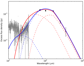
Figure 6.— SED of the $\gamma$ Dor disk derived from the imaging models. Photometric excesses are displayed with black circles and IRS excesses are in grey. The narrow rings imaging model is plotted in red and the wide belt imaging model is plotted in blue. Individual components of each model are plotted with dashed lines and the solid lines trace the total flux of each disk model. Both models require two components to reproduce the observations. The narrow rings model agrees well with the MIPS 24 µm data and places the rings at $\sim$70 and $\sim$190 AU. The wide belt imaging model that extends from $\sim$55 AU to $\sim$400 AU cannot account for the excesses at shorter wavelengths. Therefore, an additional component, a warm, narrow ring with a temperature of $\sim$225 $\pm$ 100 K, is needed and its properties are estimated from the unresolved mid-IR fluxes.

Figure 6 shows the SEDs generated for the imaging models. We have adopted the standard $\beta=1$ that is found for most debris disks (Dent et al. 2000) and fixed $\lambda_{0}=160$ µm to accommodate the SPIRE observations. Both the narrow rings and the wide belt imaging models overpredict the observed 100 µm flux. This discrepancy is also present in the SED models (Section 6.2) and therefore not an issue with the imaging models themselves. The apparent flatness of the SED between 70 and 160 µm is not characteristic of blackbody emission. More sophisticated models could explore whether this feature is due to the dust’s composition, causing broad emission features from minerals or ices, or due to the shape of the size distribution. For example, Lebreton et al. (2012) show different SED shapes for HD 181327’s debris disk for various grain compositions and size distributions.

The SED of the wide belt imaging model suggests that the excess at shorter IRS and MIPS 24 wavelengths is due to a separate component of warm dust that does not contribute to the emission at Herschel wavelengths, rather than an extension of the belt. We therefore attribute the remaining warm excess in the context of this model to a separate warm component of dust and estimate it to have a temperature of 225 K and a fractional luminosity of $4.4\times 10^{-6}$. In order to minimize the warm component’s contribution to the flux at Herschel wavelengths, we adopt a $\lambda_{0}$ of 40 µm. The parameters of this component are highly uncertain given the low significance of excess and the fluctuation of the degree of excess between different IRS reductions, and so we estimate an uncertainty of $\sim$100 K on the dust temperature. Given that the excess is apparent in all available reductions of the IRS data and MIPS photometry at 24 µm, which is even more discrepant, we are confident that it exists. The 225 K dust temperature suggests that the warm inner ring lies at $\sim$4 AU under blackbody assumptions using Equation (3). The SED modeling supports that such a warm dust temperature is present even though its physical location is poorly constrained and could lie anywhere between 2 and 12 AU given the uncertainty in temperature. Typically, the blackbody radius underestimates the true size of the disk by a factor of up to $\sim$5 (Schneider et al. 2006; Wyatt 2008; Matthews et al. 2010; Rodriguez & Zuckerman 2012; Booth et al., accepted) implying the true radius could exceed the nominal blackbody radius even further.

Modelling the SED and resolved images suggests that there are at least two dust components in $\gamma$ Dor’s debris disk. However, the resolution of the images and the SEDs are unable to distinguish between a configuration of two narrow dust rings (at 70 and 190 AU) and a configuration of a wide outer dust belt (from 54 to 400 AU) and a warm inner ring (around 4 AU).

7. Discussion

7.1. Properties of $\gamma$ Dor’s Disk

It is important to constrain where the dust is to determine the implications for a possible planetary system (Section 7.2). The modeling of the resolved images shows that the dust population probed at Herschel wavelengths could be distributed in either a wide belt and a narrow ring or two narrow rings. Figure 6 shows that both models have two dust components. The narrow rings model requires a gap between the star and the inner narrow ring at $\sim$70 AU and another gap between the inner ring and the outer narrow ring (at $\sim$190 AU). Whereas the wide belt model requires a gap between a narrow ring at $\sim$4 and the wide belt that begins at $\sim$55 AU. All models have an estimated fractional luminosity of $\sim$$10^{-5}$, within the upper limits that are typically found for other debris disks around F-type stars (Moór et al. 2011).

A common clearing mechanism that is proposed for such gaps, for example, is the presence of planets, however, they would be hard to form at such large distances from the star (e.g., Weidenschilling 2003). Therefore, the wide belt is physically more plausible since it does not require planets at such large radii. However, there are problems with the wide belt model as well, as it would require a very broad disk of dust producing planetesimals, rather than containing them in narrow rings.

The inclination of the disk is $\sim$69^∘ from a face-on orientation. This suggests that it may be aligned with the stellar equator given the inclination of $\gamma$ Dor itself is $\sim$70^∘ (Balona et al. 1996), though the orientation of the stellar inclination is not known.

The fractional luminosity of the warm inner ring of $\sim$$4.4\times 10^{-6}$ is about the maximum that can be expected to arise from collisional processes for Sun-like stars from Wyatt et al. (2007)

$$f_{\rm{max}}=0.16\times 10^{-3}~{}R^{7/3}~{}M_{*}^{-5/6}~{}L_{*}^{-1/2}~{}t_{\rm{age}}^{-1},$$ (6)

where $R$ is the dust radius in AU, $t_{\rm{age}}$ is the age of the star in Myr, $M_{*}$ is the mass of the star in solar masses, and $L_{*}$ is the luminosity of the star in solar luminosities (Section 4.1). Given $\gamma$ Dor’s age of 400 Myr, $f_{\rm{max}}$ is $2.5\times 10^{-6}$ for a dust ring at 4 AU and therefore transient events are not needed to explain this amount of hot dust.

7.2. Relation to Planetary Systems

$\gamma$ Dor is an example of how we are continuing to uncover more structure in debris disks with the resolution and sensitivity of modern observatories to move away from the simple pictures of single narrow dust rings. Observing $\gamma$ Dor with Herschel demonstrates the importance of surveys across different wavelength regimes. In the case of $\gamma$ Dor, the Spitzer and Herschel observations considered independently would give an incomplete picture of the system. Our understanding of the debris disk around $\gamma$ Dor now is that it is more complex than a single ring. We find that it is composed of dust at multiple radii by showing two extreme scenarios of this are both possible: two cool, narrow rings beyond 70 AU or a cool, wide belt beyond 55 AU and a separate warm inner ring. In both cases the dust is located between $\sim$55 AU and a few hundred AU. Depending on the exact scenario (particularly in the case of a wide belt), an additional warm component of dust (at several AU from the star) may be required to reproduce the mid-IR excess. The wide belt model with a warm inner component is much like the Solar System, although it is much younger than the Solar System, the dust is much brighter and no planets in the system have been detected yet.

$\gamma$ Dor’s multicomponent disk has implications for the possibility of the system hosting planets. For planetary systems, such as the Solar System and HR 8799, that host both planets and a debris disk, the planets are observed to lie within or between the regions of dust (Moro-Martín et al. 2010). This suggests that gaps in debris disks are good places to look for planets, particularly if the dust ring has a sharp inner edge (e.g., Fomalhaut; Kalas et al. 2005, 2008). Resonance overlap studies have shown how a planet can sculpt the inner edge of a disk (e.g., Quillen 2006, Mustill & Wyatt 2012). Migrating planets as well as planets with highly eccentric orbits can create gaps and asymmetries in debris disks (see e.g., Wyatt 2003). $\gamma$ Dor is a good target for the Atacama Large Millimeter/Submillimeter Array (ALMA) as $\gamma$ Dor’s distance is appropriate to resolve a sharp inner edge. Such observations would constrain the location of edges and therefore help distinguish between the two models presented here. If $\gamma$ Dor’s disk is indeed best described by a wide belt, the best place to look for planets would be within $\sim$55 AU of the star, where the gap between the inner ring and the wide belt is predicted. Similarly in the context of the narrow rings model a planet could be sculpting the inner ring at 70 AU and/or planets could be responsible for the gap between 70 and 190 AU.

Determining the inner edge of the disk could also have implications for the histories of the planetary systems. For example, Wyatt (2003) present a model of a Neptune-mass planet migrating from 40 to 65 AU. During the migration, the inner edge of the disk is pushed outward and objects in the disk are swept into resonances with the planet. Migration of the Solar System planets has been proposed as a possible trigger for the Late Heavy Bombardment (LHB), an epoch of intense cratering responsible for many of the features we still see on the Moon today. The LHB severely depleted the Solar system’s debris disk rendering such a system unobservable at the distance of $\gamma$ Dor within the current detection limits and available observatories (Booth et al. 2009). Although it would be unlikely to observe a planetary system while its planets are migrating, because of the short timescales over which this takes place (on the order of tens of Myr), the inner edges of debris disks and the amount of dust within them are tools to consider the Solar System’s history in the context of other planetary systems. For example, the fact that there is so much dust still around $\gamma$ Dor suggests that it has not undergone an instability as destructive as the LHB.

8. Summary and conclusions

We observed the debris disk around $\gamma$ Dor with Herschel and detect emission at all six wavelengths of PACS and SPIRE. The disk is well resolved at 70, 100, and 160 µm. It is resolved along its major axis at 250 µm; at 350 µm, the emission is point-like. The emission at 500 µm cannot be separated from that of a nearby background source. Our measurements are consistent with the disk being aligned with the stellar equator given the inclination of $\sim$70^∘ that is measured for $\gamma$ Dor based on its stellar oscillation modes (Balona et al. 1996).

The SED of the dust emission has a shape that is too broad to arise from dust at a single temperature. There is both cool dust (observable to Herschel) and warm dust (evident from IRS and MIPS 24 excesses). Similarly, the resolved images cannot be modeled by a single narrow dust ring, suggesting any temperature distribution within the cool dust arises from a radially broad distribution of dust and not dust at a single stellocentric radius with a distribution of grain properties.

We have modeled the resolved images, and therefore cool dust, at 70, 100, and 160 µm as arising from two narrow dust rings and as a single wide dust belt. The narrow rings model has two rings at large distances (70 and 190 AU) from the star and accounts for all the observed excess across mid-IR and submm wavelengths. The wide belt model has a cool, wide belt (extending from 55 to 400 AU) and accounts for far-IR and submm excesses, but not IRS and MIPS 24 excesses. Consequently, a warm inner ring must be included in this model to account for the fluxes detected at shorter wavelengths. Therefore, both models require a total of two dust components (with a total $f_{d}\sim 10^{-5}$) in the debris disk: two narrow rings of cool dust, or a wide belt of cool dust and a narrow ring of warm dust. As both models produce reasonably low residuals, the Herschel resolution is unable to distinguish which configuration best represents the $\gamma$ Dor disk.

In the context of the wide belt imaging model, the IRS and MIPS 24 excesses are attributed to a warm inner ring. Given the variability between the conclusions of different IRS observations and reductions, we do not attempt to place strong constraints on the properties of this ring, but estimate its temperature to be $\sim$225 $\pm$ 100 K and its fractional luminosity to be $\sim$$4.4\times 10^{-6}$. We derive a blackbody radius of $\sim$4 AU for the warm dust ring given a 225 K temperature, although it will be larger in the case of non-blackbody grains. The fractional luminosity of this ring is within the levels that are expected for the steady state evolution of a ring at 4 AU and therefore a transient event is not needed to explain the levels of warm dust in this system.

Planets are observed to lie between dust components in systems where both dust and planets have been observed. $\gamma$ Dor is therefore a good candidate for planet searches, particularly if planets are responsible for the lack of dust between the inner and outer dust components. The most likely region to find planets would be within 55 AU of the star, which both models support as clear of dust. Planets found beyond 55 AU would offer support to the narrow rings model as they could be responsible for the lack of dust between the two rings of cool dust.

References

- Ardila et al. (2004) Ardila, D. R., Golimowski, D. A., Krist, J. E., et al. 2004, ApJ, 617, L147
- Ardila et al. (2010) Ardila, D. R., Van Dyk, S. D., Makowiecki, W., et al. 2010, ApJS, 191, 301
- Aumann (1985) Aumann, H. H. 1985, PASP, 97, 885
- Aumann et al. (1984) Aumann, H. H., Beichman, C. A., Gillett, F. C., et al. 1984, ApJ, 278, L23
- Backman et al. (2009) Backman, D., Marengo, M., Stapelfeldt, K., et al. 2009, ApJ, 690, 1522
- Backman & Paresce (1993) Backman, D. E., & Paresce, F. 1993, in Protostars and Planets III, ed. E. H. Levy & J. I. Lunine, 1253–1304
- Balona et al. (1994) Balona, L. A., Krisciunas, K., & Cousins, A. W. J. 1994, MNRAS, 270, 905
- Balona et al. (1996) Balona, L. A., Böhm, T., Foing, B. H., et al. 1996, MNRAS, 281, 1315
- Beichman et al. (2006) Beichman, C. A., Bryden, G., Stapelfeldt, K. R., et al. 2006, ApJ, 652, 1674
- Booth et al. (2009) Booth, M., Wyatt, M. C., Morbidelli, A., Moro-Martín, A., & Levison, H. F. 2009, MNRAS, 399, 385
- Brott & Hauschildt (2005) Brott, I., & Hauschildt, P. H. 2005, in ESA Special Publication, Vol. 576, The Three-Dimensional Universe with Gaia, ed. C. Turon, K. S. O’Flaherty, & M. A. C. Perryman, 565–+
- Bryden et al. (2009) Bryden, G., Beichman, C. A., Carpenter, J. M., et al. 2009, ApJ, 705, 1226
- Chen et al. (2006) Chen, C. H., Sargent, B. A., Bohac, C., et al. 2006, ApJS, 166, 351
- Chun et al. (2008) Chun, M., Toomey, D., Wahhaj, Z., et al. 2008, in Society of Photo-Optical Instrumentation Engineers (SPIE) Conference Series, Vol. 7015, Society of Photo-Optical Instrumentation Engineers (SPIE) Conference Series
- Churcher et al. (2011) Churcher, L. J., Wyatt, M. C., Duchêne, G., et al. 2011, MNRAS, 1596
- Cutri et al. (2003) Cutri, R. M., Skrutskie, M. F., van Dyk, S., et al. 2003, 2MASS All Sky Catalog of point sources., ed. Cutri, R. M., Skrutskie, M. F., van Dyk, S., Beichman, C. A., Carpenter, J. M., Chester, T., Cambresy, L., Evans, T., Fowler, J., Gizis, J., Howard, E., Huchra, J., Jarrett, T., Kopan, E. L., Kirkpatrick, J. D., Light, R. M., Marsh, K. A., McCallon, H., Schneider, S., Stiening, R., Sykes, M., Weinberg, M., Wheaton, W. A., Wheelock, S., & Zacarias, N.
- Dent et al. (2000) Dent, W. R. F., Walker, H. J., Holland, W. S., & Greaves, J. S. 2000, MNRAS, 314, 702
- Ertel et al. (2011) Ertel, S., Wolf, S., Metchev, S., et al. 2011, A&A, 533, A132+
- Gray et al. (2006) Gray, R. O., Corbally, C. J., Garrison, R. F., et al. 2006, AJ, 132, 161
- Greaves et al. (1998) Greaves, J. S., Holland, W. S., Moriarty-Schieven, G., et al. 1998, ApJ, 506, L133
- Griffin et al. (2010) Griffin, M. J., Abergel, A., Abreu, & et al. 2010, A&A, 518, L3+
- Høg et al. (2000) Høg, E., Fabricius, C., Makarov, V. V., et al. 2000, A&A, 355, L27
- Holland et al. (1998) Holland, W. S., Greaves, J. S., Zuckerman, B., et al. 1998, Nature, 392, 788
- Ishihara et al. (2010) Ishihara, D., Onaka, T., Kataza, H., et al. 2010, A&A, 514, A1+
- Kalas et al. (2005) Kalas, P., Graham, J. R., & Clampin, M. 2005, Nature, 435, 1067
- Kalas et al. (2008) Kalas, P., Graham, J. R., Chiang, E., et al. 2008, Science, 322, 1345
- Kennedy et al. (2012) Kennedy, G. M., Wyatt, M. C., Sibthorpe, B., et al. 2012, MNRAS, 421, 2264
- Kenyon & Bromley (2004) Kenyon, S. J., & Bromley, B. C. 2004, AJ, 127, 513
- Koerner et al. (2010) Koerner, D. W., Kim, S., Trilling, D. E., et al. 2010, ApJ, 710, L26
- Krivov (2010) Krivov, A. V. 2010, Research in Astronomy and Astrophysics, 10, 383
- Lebreton et al. (2012) Lebreton, J., Augereau, J.-C., Thi, W.-F., et al. 2012, A&A, 539, A17
- Liu et al. (2010) Liu, M. C., Wahhaj, Z., & Biller, e. 2010, in Society of Photo-Optical Instrumentation Engineers (SPIE) Conference Series, Vol. 7736, Society of Photo-Optical Instrumentation Engineers (SPIE) Conference Series
- Markwardt (2009) Markwardt, C. B. 2009, in Astronomical Society of the Pacific Conference Series, Vol. 411, Astronomical Data Analysis Software and Systems XVIII, ed. D. A. Bohlender, D. Durand, & P. Dowler, 251
- Matthews et al. (2010) Matthews, B. C., Sibthorpe, B., Kennedy, G., et al. 2010, A&A, 518, L135+
- Mermilliod (2006) Mermilliod, J. C. 2006, VizieR Online Data Catalog, 2168, 0
- Moerchen et al. (2007) Moerchen, M. M., Telesco, C. M., Packham, C., & Kehoe, T. J. J. 2007, ApJ, 655, L109
- Moór et al. (2011) Moór, A., Pascucci, I., Kóspál, Á., et al. 2011, ApJS, 193, 4
- Moro-Martín et al. (2010) Moro-Martín, A., Malhotra, R., Bryden, G., et al. 2010, ApJ, 717, 1123
- Moshir et al. (1990) Moshir et al. 1990, in IRAS Faint Source Catalogue, version 2.0 (1990), 0–+
- Mustill & Wyatt (2009) Mustill, A. J., & Wyatt, M. C. 2009, MNRAS, 399, 1403
- Mustill & Wyatt (2012) —. 2012, MNRAS, 419, 3074
- Ott (2010) Ott, S. 2010, in Astronomical Society of the Pacific Conference Series, Vol. 434, Astronomical Data Analysis Software and Systems XIX, ed. Y. Mizumoto, K.-I. Morita, & M. Ohishi, 139–+
- Perryman & ESA (1997) Perryman, M. A. C., & ESA, eds. 1997, ESA Special Publication, Vol. 1200, The HIPPARCOS and TYCHO catalogues. Astrometric and photometric star catalogues derived from the ESA HIPPARCOS Space Astrometry Mission
- Phillips et al. (2010) Phillips, N. M., Greaves, J. S., Dent, W. R. F., et al. 2010, MNRAS, 403, 1089
- Pilbratt et al. (2010) Pilbratt, G. L., Riedinger, J. R., Passvogel, T., et al. 2010, A&A, 518, L1+
- Poglitsch et al. (2010) Poglitsch, A., Waelkens, C., Geis, N., et al. 2010, A&A, 518, L2+
- Quillen (2006) Quillen, A. C. 2006, MNRAS, 372, L14
- Reidemeister et al. (2011) Reidemeister, M., Krivov, A. V., Stark, C. C., et al. 2011, A&A, 527, A57+
- Rhee et al. (2007) Rhee, J. H., Song, I., Zuckerman, B., & McElwain, M. 2007, ApJ, 660, 1556
- Rieke et al. (2005) Rieke, G. H., Su, K. Y. L., Stansberry, J. A., et al. 2005, ApJ, 620, 1010
- Roccatagliata et al. (2009) Roccatagliata, V., Henning, T., Wolf, S., et al. 2009, A&A, 497, 409
- Rodriguez & Zuckerman (2012) Rodriguez, D. R., & Zuckerman, B. 2012, ApJ, 745, 147
- Schaller et al. (1992) Schaller, G., Schaerer, D., Meynet, G., & Maeder, A. 1992, A&AS, 96, 269
- Schneider et al. (2006) Schneider, G., Silverstone, M. D., Hines, D. C., et al. 2006, ApJ, 650, 414
- Sibthorpe et al. (2010) Sibthorpe, B., Vandenbussche, B., Greaves, J. S., et al. 2010, A&A, 518, L130+
- Stock et al. (2010) Stock, N. D., Su, K. Y. L., Liu, W., et al. 2010, ApJ, 724, 1238
- Su et al. (2005) Su, K. Y. L., Rieke, G. H., Misselt, K. A., et al. 2005, ApJ, 628, 487
- Su et al. (2009) Su, K. Y. L., Rieke, G. H., Stapelfeldt, K. R., et al. 2009, ApJ, 705, 314
- van Altena et al. (1995) van Altena, W. F., Lee, J. T., & Hoffleit, E. D. 1995, The general catalogue of trigonometric [stellar] parallaxes
- van Leeuwen (2007) van Leeuwen, F. 2007, A&A, 474, 653
- Vican (2012) Vican, L. 2012, AJ, 143, 135
- Weidenschilling (2003) Weidenschilling, S. J. 2003, Icarus, 165, 438
- Wyatt (2003) Wyatt, M. C. 2003, ApJ, 598, 1321
- Wyatt (2008) —. 2008, ARA&A, 46, 339
- Wyatt et al. (2005) Wyatt, M. C., Greaves, J. S., Dent, W. R. F., & Coulson, I. M. 2005, ApJ, 620, 492
- Wyatt et al. (2007) Wyatt, M. C., Smith, R., Greaves, J. S., et al. 2007, ApJ, 658, 569
- Wyatt et al. (2012) Wyatt, M. C., Kennedy, G., Sibthorpe, B., et al. 2012, MNRAS, 424, 1206