Rare events and scaling properties in field-induced anomalous dynamics

Abstract

We show that, in a broad class of continuous time random walks (CTRW), a small external field can turn diffusion from standard into anomalous. We illustrate our findings in a CTRW with trapping, a prototype of subdiffusion in disordered and glassy materials, and in the Lévy walk process, which describes superdiffusion within inhomogeneous media. For both models, in the presence of an external field, rare events induce a singular behavior in the originally Gaussian displacements distribution, giving rise to power-law tails. Remarkably, in the subdiffusive CTRW, the combined effect of highly fluctuating waiting times and of a drift yields a non-Gaussian distribution characterized by long spatial tails and strong anomalous superdiffusion.

1 Introduction

Large fluctuations and rare events play an important role in many physical processes. Their contribution strongly influences physical observables in laser cooling [1], liposome diffusion [2], heteropolymers [3], chaotic systems [4] and non-equilibrium relaxation [5, 6]. In these systems, heterogeneous spatial structures or temporal inhomogeneities can give rise to anomalous transport: the mean square displacement (MSD) of a tagged particle is not linear in time, $\langle x^{2}(t)\rangle\sim t^{2/\gamma}$, with $\gamma\neq 2$, and one observes either subdiffusion, $\gamma>2$, or superdiffusion, $\gamma<2$. However, when the fluctuations in the microscopic dynamics are not too large, i.e. the tails of their probability distributions decay fast enough, anomalous transport is suppressed, and standard diffusion can occur also in the presence of inhomogeneities. In these subtle situations, detecting large deviations and establishing the heterogeneous nature of the underlying microscopic dynamics can be difficult. We show here that the presence of an arbitrary small external field can induce an anomalous growth of fluctuations even when the unperturbed behavior remains Gaussian. This is an example, similar to others recently pointed out in [7, 8], of how the response to an external field may feature anomalous effects in the case of nonlinear dynamics. These topics can find application for instance in probe-based microrheology, for the study of the motion of a tracer particle in a disordered system when an external force is applied [9]. We remark that, for our heterogeneous systems, the Einstein relation established in [10, 11, 12, 13, 14] proves a proportionality between $\langle x^{2}(t)\rangle$ and the drift $\langle x(t)\rangle_{\epsilon}$, where $\langle\dots\rangle_{\epsilon}$ denotes the average over the process with an external field $\epsilon$.

For standard diffusion governed by the Fick’s law, the Gaussian form of the probability density function (PDF) of displacements at time $t$, $P_{0}(x,t)$, is not altered by the presence of a field $\epsilon$:

$$P_{\epsilon}(x,t)\simeq\frac{1}{\sqrt{4\pi Dt}}\exp\left[-\frac{(x-v_{\epsilon}t)^{2}}{4Dt}\right],$$ (1)

where $D$ is the diffusion coefficient. The field induces a finite drift, $\langle x(t)\rangle_{\epsilon}/t\equiv v_{\epsilon}\not=0$, and a typical displacement $l_{T}(t)$, defined as the maximum of the PDF, growing as $l_{T}(t)=v_{\epsilon}t$.

When the microscopic dynamics is characterized by large space inhomogeneities and/or several time scales, the action of a field can induce relevant deviations from the Gaussian behavior [5]. We study here the properties of $P_{\epsilon}(x,t)$ in the presence of a field for models with scale invariant distribution of trapping times and with scale invariant distributions of displacements. We consider a continuous time random walk (CTRW) [5] with trapping, where a Brownian particle is trapped for a time interval distributed according to a given PDF, which shows subdiffusive dynamics and mimics the slow activated dynamics of complex fluids [15]. It embeds the waiting time distribution

$$p_{\alpha}(\tau)\sim\tau^{-(\alpha+1)},$$ (2)

where $\alpha>0$ is the exponent characterizing the slow decay of time distribution.

Fat tails also occur in displacements distribution, and in particular they characterize the Lévy-like motion in heterogeneous materials [16, 17, 18, 19, 20], or in turbulent flow [21], where transport is realized through increments of size $l$ with distribution $p_{\alpha}(l)\sim l^{-(1+\alpha)}$ [22, 23, 24] and superdiffusive dynamics can occur. Interestingly, it has been recently found [25] that even in a nearly arrested granular assembly the displacements of grains follow a Lévy distribution, producing an unexpected superdiffusive dynamics. Moreover, as predicted in [5], and found in numerical simulations of complex liquids [26, 27], a superdiffusive dynamics may be induced by an external field also in trap-like disordered systems.

For vanishing field, i.e. $\epsilon=0$, if the tails of the steps and waiting times distributions decay slowly enough, both the CTRW with trapping and the Lévy walk lead to anomalous transport, subdiffusive and superdiffusive, respectively. In these regimes, motion is largely influenced by rare events and $P_{0}(x,t)$ is not Gaussian, presenting, up to distances of order $\ell(t)$, the generalized scaling form $P_{0}(x,t)\sim t^{-1/z}F(x/t^{1/z})$, where $\ell(t)\sim t^{1/z}$ is the scaling length. In the case of fast asymptotic decay of $F(y)$, the behavior of the moments is given by $\langle x^{n}(t)\rangle\sim\ell^{n}(t)$. However, due to rare events, also $F(y)$ can present a slow decay. In this case the scaling is broken for $x\gg\ell(t)$ and the system can feature “strong” anomalous behavior, i.e. the moments of the distribution are not a power of $\ell(t)$ [28]. On the other hand, when the fluctuations of $p_{\alpha}(\tau)$ or of $p_{\alpha}(l)$ are not too large, $P_{0}(x,t)$ is Gaussian.

In this paper we show that, remarkably, the presence of a drift can induce an anomalous non-Gaussian dynamic even for regimes where equilibrium measurements show a standard diffusive behavior. By solving the master equations of the two processes mentioned above in the one-dimensional case, we determine the PDF in the presence of an external field. We evidence that, as expected, in the region of anomalous transport, the distributions are very sensitive to the presence of a drift. More surprisingly, in the regimes where the form of the distribution is simply Gaussian at equilibrium, we find that the field can induce a non-Gaussian shape of $P_{\epsilon}(x,t)$. In the CTRW with trapping, we identify an interval of values of $\alpha$ where the combined effect of highly fluctuating waiting times and drift gives rise to a perturbed non-Gaussian PDF spreading out superdiffusively. Our main result is that, even when drift and diffusion are standard, an underlying anomalous behavior can be singled out by studying the response to external perturbations. An arbitrary small field can induce a transition from standard Gaussian diffusion to a strong anomalous one.

2 Models and scaling hypotheses

In the CTRW with trapping, a particle moves with probability $1/2$ from $x$ to $x\pm\delta_{0}$, where $\delta_{0}$ is constant. The main results do not change with a symmetric distribution of $\delta_{0}$ with finite variance. Between successive steps, the particle waits for a time $\tau$ extracted from the distribution (2). In the Lévy walk model again there are time intervals of duration $\tau$ extracted from the distribution (2), but the particle, during each time lag, moves at a constant velocity $v$, chosen from a symmetric distribution with finite variance, and performs displacements $\tau v$. Here we consider $v=\pm v_{0}$ with equal probability and $v_{0}$ constant. In both models we introduce a lower cutoff $\tau_{0}=1$ in the distribution (2) so that, taking into account of the normalization, we have $p_{\alpha}(\tau)=\alpha\Theta(\tau-1)\tau^{-(1+\alpha)}$, where $\Theta(x)$ is the Heaviside step function. The value of $\tau_{0}$ does not change the behavior of the model apart from a suitable rescaling of the constants.

In the CTRW with trapping, the external field is implemented by unbalancing the jump probabilities, i.e. setting to $(1\pm\epsilon)/2$ the probability of jumping to the right or to the left, respectively. For the Lévy walk, in [32, 33] it has been shown that the natural way to drive the system out of equilibrium is to apply an external field accelerating the particle during the walk, so that the distance traveled after a scattering event is $\delta=\pm v_{0}\tau+\epsilon\tau^{2}$. In the following we will consider a positive bias $\epsilon>0$.

Inspired by the Gaussian case, the simplest generalization of Eq. (1) for $\epsilon\neq 0$ is:

$$P_{\epsilon}(x,t)\sim t^{-1/z}F[(x-v_{\epsilon}t)/t^{1/z}].$$ (3)

When $\epsilon=0$, the left-right symmetry implies that $v_{\epsilon}=0$ and $F(y)$ is an even function. In systems with power-law distributions, Eq. (3) is made slightly more complex by the occurrence of field-induced rare events: in Lévy walks a fat tail due to large displacements in the direction of the field must be considered, whereas in the CTRW with trapping we find a distribution uniformly shifting in time in the direction of the field, plus an algebraic tail for small values of $x$, originated from particles with a large trapping time. In both situations the simple scaling form of Eq. (3) leads to inconsistencies in the behavior of the moments of arbitrary order $\langle x^{n}(t)\rangle_{\epsilon}$. Indeed there is a cut-off in the largest distance from the peak of the distribution at which a particle can be found in both models. In the Lévy walk at time $t$, there can be no displacement exceeding $v_{0}t+\epsilon t^{2}$, so that for large times we have:

$$P_{\epsilon}(x,t)\sim t^{-1/z}F[(x-v_{\epsilon}t)/t^{1/z}]~{}\Theta\left(\epsilon t^{2}-x\right).$$ (4)

In the CTRW with trapping, the factor $\Theta(\epsilon t^{2}-x)$ in Eq. (4) has to be replaced by $\Theta(x)$, which cuts off the power-law tail due to particles with large persistence time at the origin. In Eq. (4) there are three characteristic lengths: the length-scale of the peak displacement, $l_{T}(t)\sim t$; the length-scale for the collapse of the function, $l(t)\sim t^{1/z}$; the length-scale of the largest displacement from the peak of the distribution, $l_{e}(t)\sim t^{2}$.

3 Solution of the master equation for the CTRW with trapping

The scaling arguments (4) can be proved by writing the master equations relating, at two subsequent scattering events, $P_{\epsilon}(x,t)$ with the function $Q_{\epsilon}(x,t)$, i.e. the probability of being scattered in $x$ at time $t$ [34, 31]. For the CTRW with trapping we have:

$$Q_{\epsilon}(x,t)=\int_{0}^{t}\left[\frac{1+\epsilon}{2}Q_{\epsilon}(x-\delta_{0},t-t^{\prime})+\frac{1-\epsilon}{2}Q_{\epsilon}(x+\delta_{0},t-t^{\prime})\right]p_{\alpha}(t^{\prime})dt^{\prime}+\delta(t)\delta(x)$$ (5)

with

$$P_{\epsilon}(x,t)=\int_{0}^{t}Q_{\epsilon}(x,t-t^{\prime})\int_{t^{\prime}}^{\infty}p_{\alpha}(\tau)d\tau dt^{\prime},$$ (6)

where $\delta(x)$ is the Dirac delta. We solve Eq. (5), taking the time and space Fourier transform, $P_{\epsilon}(x,t)\to\tilde{P}_{\epsilon}(k,\omega)$ and $Q_{\epsilon}(x,t)\to\tilde{Q}_{\epsilon}(k,\omega)$. From Eq. (5) we obtain

$$\tilde{Q}_{\epsilon}(k,\omega)=\frac{1}{1-[\cos(k\delta_{0})+i\epsilon\sin(k\delta_{0})]\int p_{\alpha}(t^{\prime})e^{i\omega t^{\prime}}dt^{\prime}}.$$ (7)

Then, taking the Fourier transform of Eq. (6) we get

$$\tilde{P}_{\epsilon}(k,\omega)=\tilde{Q}_{\epsilon}(k,\omega)\int e^{i\omega t^{\prime}}\int_{t^{\prime}}^{\infty}p_{\alpha}(\tau)d\tau dt.^{\prime}$$ (8)

We then substitute expression Eq. (7) into Eq. (8) and finally consider the asymptotic regimes where simultaneously $k\to 0$ and $\omega\to 0$, neglecting subleading terms.

For $\epsilon=0$, the results are well known [34]:

$$\tilde{P}_{0}(k,\omega)\approx\begin{cases}\frac{C_{1}\omega^{\alpha-1}}{(\delta_{0}k)^{2}/2+C_{2}\omega^{\alpha}}\qquad\mathrm{if}\qquad 0<\alpha<1\\ \frac{\langle t\rangle}{(\delta_{0}k)^{2}/2+i\langle t\rangle\omega}\qquad\mathrm{if}\qquad\alpha>1,\\ \end{cases}$$ (9)

where $\langle t^{p}\rangle=\int t^{p}p_{\alpha}(t)dt$. The complex number $C_{i}$ depends on the sign of $\omega$:

$$C_{1}(\alpha)=\int_{0}^{\infty}\frac{\cos(t)}{t^{\alpha}}dt+i\ {\rm sign}(\omega)\int_{0}^{\infty}\frac{\sin(t)}{t^{\alpha}}dt$$ (10)

and

$$C_{2}(\alpha)=i\ {\rm sign}(\omega)\ C_{1}(\alpha)=-\int_{0}^{\infty}\frac{\sin(t)}{t^{\alpha}}dt+i\ {\rm sign}(\omega)\int_{0}^{\infty}\frac{\cos(t)}{t^{\alpha}}dt,$$ (11)

with $0<\alpha<1$. For $\alpha>1$, Eq. (9) corresponds to standard diffusion, while for $0<\alpha<1$ the Gaussianity is broken and the dynamics is characterized by a subdiffusive scaling length $\ell(t)\sim t^{\alpha/2}$.

For $\epsilon\not=0$ we obtain in the asymptotic regime:

$$\tilde{P}_{\epsilon}(k,\omega)\approx\begin{cases}\frac{C_{1}\omega^{\alpha-1}}{i\epsilon\delta_{0}k+C_{2}\omega^{\alpha}}\qquad\mathrm{if}\qquad 0<\alpha<1\\ \frac{\langle t\rangle}{i(\epsilon\delta_{0}k+\langle t\rangle\omega)+C_{3}\omega^{\alpha}}\qquad\mathrm{if}\qquad 1<\alpha<2\\ \frac{\langle t\rangle}{(\delta_{0}k)^{2}/2+i(\epsilon\delta_{0}k+\langle t\rangle\omega)}\qquad\mathrm{if}\qquad\alpha>2.\end{cases}$$ (12)

where $C_{3}(\alpha)=-\frac{C_{1}(\alpha-1)}{\alpha-1}$. The immaginary parts of the coefficients $C_{1}$, $C_{2}$ and $C_{3}$ depend on the sign of $\omega$, so that $P_{\epsilon}(x,t)$ is a real function. The numerical inverse Fourier transform of $\tilde{P}_{\epsilon}(k,\omega)$ can be easily computed and it is in very good agreement with the results of simulations, as shown in Fig. 1 for $\alpha=1.5$. Notice that the space inverse Fourier transform can be performed explicitly from Eqs. (12), yielding a $\Theta(x)$ function in the $P_{\epsilon}(x,t)$, as expected from the arguments following Eq. (4). In particular, for $1<\alpha<2$ we get:

$$\tilde{P}_{\epsilon}(x,t)=\langle t\rangle\Theta(x)\int e^{-i\omega(x/(\epsilon\delta_{0})\langle t\rangle-t)-C_{3}|\omega^{\alpha}|x/(\epsilon\delta_{0})}d\omega.$$ (13)

.

We remark that for $|x-v_{\epsilon}t|\lessapprox\ell(t)$ all the regimes follow the general scaling pictures of Eq. (3). In particular, for $\alpha>2$, the standard response of a diffusive system is reproduced: $F(y)$ is a Gaussian moving at constant velocity $v_{\epsilon}=\epsilon\delta_{0}/\langle t\rangle$. For $0<\alpha<1$, where Gaussianity is broken already at equilibrium, the characteristic length grows as $\ell(t)\sim t^{\alpha}$. We notice that $v_{\epsilon}=0$, and hence a rigid motion of the probability with constant velocity is not observed. Comparing Eqs. (9) and (12), a singular behavior at $\epsilon=0$ is evident: $F(y)$ changes its shape, as soon as $\epsilon\not=0$. The scaling function becomes asymmetric with respect to the origin $y=0$, giving rise to an overall motion in the direction of the external field. For $1/2<\alpha<1$, one finds a superdiffusive behavior induced by the field, as discussed in [5]. In this case, due to the fast asymptotic decay of $F(y)$, the behavior of moments is $\langle x^{n}(t)\rangle_{\epsilon}\sim\ell^{n}(t)$, which is an example of weak anomalous diffusion [28].

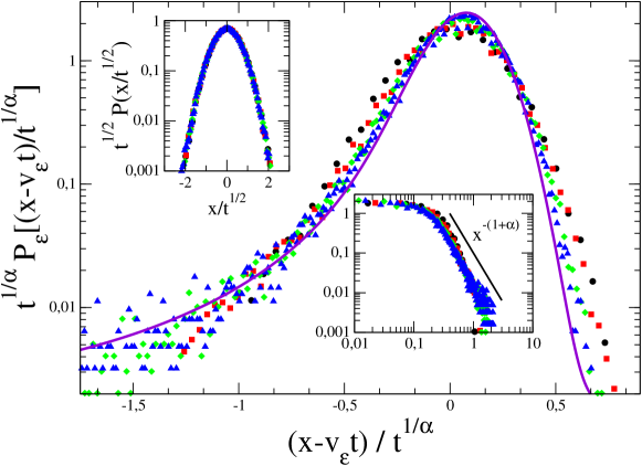
Figure 1: (color online) Collapse of the PDFs of the CTRW with trapping, for $\alpha=1.5$ and field $\epsilon=0.15$ according to Eq. (3) with velocity $v_{\epsilon}=0.1$. Symbols correspond to different times: $t=10^{3}$ ($\bullet$), $t=2\cdot 10^{3}$ ($\blacksquare$), $t=5\cdot 10^{3}$ ($\blacklozenge$), and $t=10^{4}$ ($\blacktriangle$). The continuous line represents the numerical inverse Fourier transform of Eq. (12). Central inset: same data of the main figure in log-log scale, as function of $|x-v_{\epsilon}t|$. Notice the power law behavior $P_{\epsilon}(x,t)\sim x^{-(1+\alpha)}$. Top left inset: collapse of the PDF for $\alpha=1.5$ with zero drift, $\epsilon=0$. Notice the simple Gaussian behavior, $\ell(t)\sim t^{1/2}$, in agreement with Eq. (9).

The most intriguing case is for $1<\alpha<2$, where the presence of the field turns diffusion from standard into strong anomalous [29]: the scaling function moves at constant velocity $v_{\epsilon}=\epsilon\delta_{0}/\langle t\rangle$, however the shape of $F(y)$ is not Gaussian, and it develops a power-law tail. In Fig. 1 we show the collapse of the PDFs at different times, according to the scaling in Eq. (3), for the case $\alpha=1.5$ with and without external field (see inset). The numerical inverse Fourier transform of Eq. (12) shows that the analytical calculations of the asymptotic regime are able to capture the shape of the distribution and the scaling length $l(t)\sim t^{1/z}$, with $z=\alpha<2$. The superdiffusive spreading of the PDF is triggered by rare events induced by long waiting times. In particular, the exponent of the left power-law tail of the $P_{\epsilon}(x,t)$ is obtained from the probability, that, up to a time $t$, a particle remained at rest for an interval $\tau$ such that $v_{\epsilon}\tau=\xi$, namely $P_{\epsilon}(\xi=|x-v_{\epsilon}t|,t)\sim t\xi^{-(1+\alpha)}\Theta(vt-\xi)$. Notice that the power-law tail is suppressed for $x<0$ by the function $\Theta(x)$, because the probability of finding particles with a negative displacement is zero, due to the positive field. Following the above arguments one obtains for the MSD around the peak of the distribution: $\langle\xi^{2}(t)\rangle_{\epsilon}\sim t^{3-\alpha}\neq\ell^{2}(t)\sim t^{2/\alpha}$.

4 Solution of the master equation for the Lévy walk

Let us now consider the Lévy walk. The master equation is:

$$Q_{\epsilon}(x,t)=\int_{0}^{t}\frac{1}{2}\left[Q_{\epsilon}(x-v_{0}t^{\prime}-\epsilon t^{\prime 2},t-t^{\prime})+Q_{\epsilon}(x+v_{0}t^{\prime}-\epsilon t^{\prime 2},t-t^{\prime})\right]p_{\alpha}(t^{\prime})dt^{\prime}+\delta(t)\delta(x)$$ (14)

with

$$P_{\epsilon}(x,t)=\int_{0}^{t}\frac{1}{2}\left[Q_{\epsilon}(x-v_{0}t^{\prime}-\epsilon t^{\prime 2},t-t^{\prime})+Q_{\epsilon}(x+v_{0}t^{\prime}-\epsilon t^{\prime 2},t-t^{\prime})\right]\int_{t^{\prime}}^{\infty}p_{\alpha}(\tau)d\tau dt^{\prime},$$ (15)

where $p_{\alpha}(\tau)$ is now the distribution of flight times. Analogously to Eq. (5), we first solve Eq. (14) in Fourier space and then we insert the result in Eq. (15), taking the limit of small $k$ and $\omega$. For $\epsilon=0$, the Fourier transform $\tilde{P}_{0}(k,\omega)$ reads [30, 31]:

$$\tilde{P}_{0}(k,\omega)=\begin{cases}\frac{\omega^{\alpha-1}f(k/\omega)}{C_{4}v_{0}^{\alpha}k^{\alpha}+C_{2}\omega^{\alpha}}\qquad\mathrm{if}\qquad 0<\alpha<1\\ \frac{\langle t\rangle}{C_{4}v_{0}^{\alpha}k^{\alpha}+i\langle t\rangle\omega}\qquad\mathrm{if}\qquad 1<\alpha<2\\ \frac{\langle t\rangle}{v_{0}^{2}\langle t^{2}\rangle k^{2}/2+i\langle t\rangle\omega}\qquad\mathrm{if}\qquad\alpha>2\\ \end{cases}$$ (16)

where $C_{4}$ is a real coefficient that depends on $\alpha$, and $f(k/\omega)$ is a regular complex function with $f(0)=iC_{1}$ and $f(x)\sim x^{\alpha-1}$ for $x\to\infty$. In this case, standard Gaussian diffusion is recovered for $\alpha>2$, while for $1<\alpha<2$ and $0<\alpha<1$ the non-Gaussian propagator corresponds to a superdiffusive ($\ell(t)\sim t^{1/\alpha}$) and a ballistic ($\ell(t)\sim t$) motion, respectively.

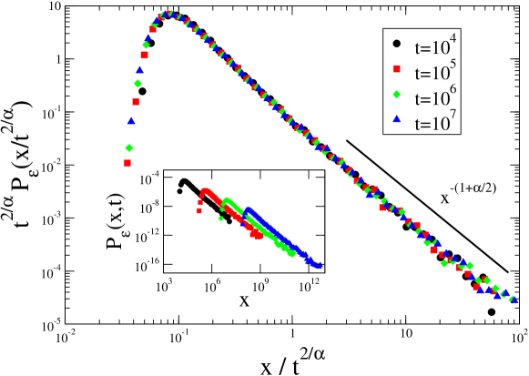
Figure 2: (color online) Collapse of PDFs with the scaling $t^{2/\alpha}P_{\epsilon}(x/t^{2/\alpha})$, for the Lévy walk with exponent $\alpha=1.5$ and field $\epsilon=0.25$. Inset: $P_{\epsilon}(x,t)$ at different times. Notice that the approximation $(x-v_{\epsilon}t)/t^{2/\alpha}\sim x/t^{2/\alpha}$ works very well asymptotically.

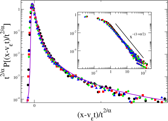
Figure 3: (color online) Collapse of the PDFs with the scaling $t^{2/\alpha}P_{\epsilon}[(x-v_{\epsilon}t)/t^{2/\alpha}]$, for the Lévy walk with exponent $\alpha=2.5$ and field $\epsilon=0.25$, with $v_{\epsilon}=0.38$. Symbols correspond to different times: $t=1.6\cdot 10^{4}$ ($\bullet$), $t=3.2\cdot 10^{4}$ ($\blacksquare$), $t=6.4\cdot 10^{4}$ ($\blacklozenge$), and $t=1.28\cdot 10^{5}$ ($\blacktriangle$). The line represents the numerical inverse Fourier transform of Eq. (17). Inset: same data of the main figure in log-log scale.

For $\epsilon\neq 0$ in the asymptotic regimes of small $k$ and $\omega$ we obtain:

$$\tilde{P}_{\epsilon}(k,\omega)\approx\begin{cases}\frac{\omega^{\alpha-1}g(k^{1/2}/\omega)}{C_{5}\epsilon^{\alpha/2}k^{\alpha/2}+C_{2}\omega^{\alpha}}\qquad\mathrm{if}\qquad 0<\alpha<1\\ \frac{\langle t\rangle}{C_{5}\epsilon^{\alpha/2}k^{\alpha/2}+i\langle t\rangle\omega}\qquad\mathrm{if}\qquad 1<\alpha<2\\ \frac{\langle t\rangle}{C_{5}\epsilon^{\alpha/2}k^{\alpha/2}+i(\epsilon\langle t^{2}\rangle k+\langle t\rangle\omega)}\qquad\mathrm{if}\qquad 2<\alpha<4\\ \frac{\langle t\rangle}{\langle t^{2}\rangle v_{0}^{2}k^{2}/2+i(\epsilon\langle t^{2}\rangle k+\langle t\rangle\omega)}\qquad\mathrm{if}\qquad\alpha>4\end{cases}$$ (17)

where $C_{5}(\alpha)$ is a complex number whose immaginary part depends on the sign of $\omega$ and $g(x)$ is a regular complex function with $g(0)=iC_{5}$ and $g(x)\sim x^{\alpha-1}$ for $x\to\infty$.

Retaining only the leading terms in $k$ and $\omega$ in the previous expressions and performing the inverse Fourier transform in space and time, one obtains a PDF of displacements in very good agreement with the numerical simulations (see Fig. 3). However, the asymptotic approximation looses the cut-off on displacements at a finite time. Indeed, at each time $t$, the largest allowed displacement is $x=v\tau+\epsilon\tau^{2}\sim\epsilon\tau^{2}$, corresponding to the rare event of a particle never colliding up to $\tau=t$, and this bound necessarily requires for the $\Theta(\epsilon t^{2}-x)$ in Eq. (4).

We find that for $\alpha>4$ Eq. (17) describes a Gaussian distribution, moving at velocity $v_{\epsilon}=\epsilon\langle t^{2}\rangle/\langle t\rangle$. For $\alpha<2$, the rigid translation of the scaling function is subdominant ($v_{\epsilon}t\ll t^{2/\alpha}$) and the global effect of the field is a strong asymmetry of $F(y)$ (see Fig. 2). In this case the scaling length grows in super-ballistic way, i.e. $z=1/2$ (linearly accelerated motion) for $0<\alpha<1$ and $z=\alpha/2$ for $1<\alpha<2$. Finally, for $2<\alpha<4$ the drift with velocity $v_{\epsilon}$ becomes relevant, but the scaling function is still not Gaussian due to an emerging power-law tail which produces a strong anomalous superdiffusive behavior. The remarkable feature for the Lévy walk with $2<\alpha<4$ is that, similarly to the CTRW with $1<\alpha<2$, the field $\epsilon$ produces a power-law tail otherwise not present in the zero-field Gaussian distribution (see Fig. 3). Moreover the scaling length $\ell(t)$ which yields the collapse of the PDFs does not govern the behavior of moments, $\langle x^{n}(t)\rangle_{\epsilon}\neq\ell^{n}(t)$. The algebraic tail of $P_{\epsilon}(x,t)$ at large time can be obtained from the distribution of flight times by changing variables: one finds $P_{\epsilon}(x,t)\sim x^{-(1+\alpha/2)}$, yielding the asymptotic behavior readable in Figs. 2 and 3. This power-law behavior, together with the cut-off $\Theta(\epsilon t^{2}-x)$, yields the MSD around the peak of the distribution: $\langle[\delta x(t)]^{2}\rangle_{\epsilon}=\langle x^{2}(t)\rangle_{\epsilon}-\langle x(t)\rangle^{2}_{\epsilon}\sim t^{5-\alpha}\neq\ell(t)^{2}\sim t^{4/\alpha}$, showing that a single scaling length cannot capture the behavior of all moments.

5 Conclusion

We have presented results for the CTRW with trapping and the Lévy walk in the presence of currents. At variance with standard Gaussian systems, the field, even arbitrarily small, significantly modifies the scaling properties of the PDF of displacements, introducing a new length-scale related to rare events. Beyond the principal scaling length of the distribution $\ell(t)$ and that related to the rigid shift, $\ell_{T}(t)$, one must also consider the typical length introduced by the cut-off of the power-law tail, $\ell_{e}(t)$, necessary for the calculation of higher order moments. This is how rare events induce the strong anomalous behavior. The change in transport properties in the presence of an external field represents a valuable probe to unveil the underlying dynamical structure of the system. Field-induced anomalous behavior highlights the importance of rare and large fluctuations in regimes where the diffusional properties are apparently standard.

Our results have been derived in a one-dimensional model, both for the CTRW with trapping and the Lévy walk. However, we expect that the main effects should be valid also in realistic experimental three dimensional samples, due to the decoupling of the motion in the direction of the field and in the orthogonal direction. Hence, we expect to observe the same behavior along the applied field, while the motion in the perpendicular directions should be described by the CTRW equations without fields i.e. $P_{0}(x,t)$.

References

References

- [1] F. Bardou, J.-P. Bouchaud, A. Aspect, and C. Cohen-Tannoudji, 2001 Lévy Statistics and Laser Cooling: How Rare Events Bring Atoms to Rest (Cambridge University Press, Cambridge).
- [2] B. Wang, J. Kuo, S. C. Bae, and S. Granick, 2012 Nature Materials 485 11 .
- [3] L. H. Tang and H. Chaté, 2001 Phys. Rev. Lett. 86 830.
- [4] A. D. Sánchez, J. M. López, M. A. Rodríguez, and M. A. Matías, 2004 Phys. Rev. Lett. 92 204101.
- [5] J.-P. Bouchaud and A. Georges, 1990 Phys. Rep. 195 127.
- [6] P. Ribière, P. Richard, R. Delannay, D. Bideau, M. Toiya, and W. Losert, 2005 Phys. Rev. Lett. 95 268001.
- [7] O. Bénichou, C. Mejía-Monasterio, and G. Oshanin, 2013 Phys. Rev. E 87 020103(R).
- [8] O. Bénichou, P. Illien, C. Mejía-Monasterio, and G. Oshanin, 2013 J. Stat. Mech. P05008.
- [9] L. G. Wilson and W. C. K. Poon, 2011 Phys. Chem. Chem. Phys. 13 10617.
- [10] E. Barkai and V. Fleurov, 1998 Phys. Rev. E 58 1296.
- [11] S. Jespersen, R. Metzler, and H. C. Fogedby, 1999 Phys. Rev. E 59 2736.
- [12] D. Villamaina, A. Sarracino, G. Gradenigo, A. Puglisi and A. Vulpiani, 2011 J. Stat. Mech. L01002.
- [13] U. Marini Bettolo Marconi, A. Puglisi, L. Rondoni, and A. Vulpiani, 2008 Phys. Rep. 461 111.
- [14] O. Bénichou, P. Illien, G. Oshanin, and R. Voituriez, 2013 Phys. Rev. E 87 032164.
- [15] L. Angelani, R. Di Leonardo, G. Parisi, and G. Ruocco, 2001 Phys. Rev. Lett. 87 055502.
- [16] P. Levitz, 593 Europhys. Lett. 39 (1997).
- [17] D. ben-Avraham and S. Havlin, 2004 Diffusion and Reactions in Fractals and Disordered Systems (Cambridge University Press (Cambridge University Press).
- [18] R. Burioni, L. Caniparoli, and A. Vezzani, 2012 Phys. Rev. E 81 060101.
- [19] P. Buonsante, R. Burioni and A. Vezzani, 2011 Phys. Rev. E 84 021105.
- [20] O. Bénichou, C. Loverdo, M. Moreau, and R. Voituriez, 2011 Rev. Mod. Phys. 83 81.
- [21] M. F. Shlesinger and J. Klafter, 1985 Phys. Rev. Lett. 54 2551.
- [22] P. Barthelemy, J. Bertolotti and D. S. Wiersma, 2008 Nature 453 495.
- [23] J. Bertolotti, K. Vynck, L. Pattelli, P. Barthelemy, S. Lepri, and D. S. Wiersma, 2012 Adv. Funct. Mat. 20 965.
- [24] R. Klages, G. Radons and I. M. Sokolov (Eds.), 2008 Anomalous Transport: Foundations and Applications (Wiley, VCH Berlin).
- [25] F. Lechenault, R. Candelier, O. Dauchot, J.-P. Bouchaud and G. Biroli, 2012 Soft Matter 6 3059.
- [26] D. Winter, J. Horbach, P. Virnau and K. Binder, 2012 Phys. Rev. Lett.108 028303.
- [27] C. F. E. Schroer and A. Heuer, 2013 Phys. Rev. Lett. 110 067801.
- [28] P. Castiglione, A. Mazzino, P. Muratore-Ginanneschi, and A. Vulpiani, 1999 Physica D 134 75.
- [29] M. Shlesinger, 1974 J. Stat. Phys. 10 421
- [30] M. Zumofen and J. Klafter, 1993 Phys. Rev. E 47 851.
- [31] M. Schmiedeberg, V. Y. Zaburdaev, and H. Stark, 2009 J. Stat. Mech. P12020.
- [32] I. M. Sokolov and R. Metzler, 2003 Phys. Rev. E 67 010101(R).
- [33] G. Gradenigo, A. Sarracino, D. Villamaina, and A. Vulpiani, 2012 J. Stat. Mech. L06001.
- [34] J. Klafter and I. M. Sokolov, 2011 First steps in random walks (Oxford University Press, Oxford).