A new approach to crushing
3-manifold triangulations

Abstract.

The crushing operation of Jaco and Rubinstein is a powerful technique in algorithmic 3-manifold topology: it enabled the first practical implementations of 3-sphere recognition and prime decomposition of orientable manifolds, and it plays a prominent role in state-of-the-art algorithms for unknot recognition and testing for essential surfaces. Although the crushing operation will always reduce the size of a triangulation, it might alter its topology, and so it requires a careful theoretical analysis for the settings in which it is used.

The aim of this short paper is to make the crushing operation more accessible to practitioners, and easier to generalise to new settings. When the crushing operation was first introduced, the analysis was powerful but extremely complex. Here we give a new treatment that reduces the crushing process to a sequential combination of three “atomic” operations on a cell decomposition, all of which are simple to analyse. As an application, we generalise the crushing operation to the setting of non-orientable 3-manifolds, where we obtain a new practical and robust algorithm for non-orientable prime decomposition. We also apply our crushing techniques to the study of non-orientable minimal triangulations.

1. Introduction

Algorithms in computational 3-manifold topology often exhibit an enormous gap between theory and practice. Theoretical solutions are now known for a large number of difficult 3-dimensional topological problems, ranging from smaller problems such as recognising the unknot [13] or recognising the 3-sphere [25] through to decomposition into geometric pieces [18] and of course the full homeomorphism (or “topological equivalence”) problem [14, 15, 22]. Although these results are of high significance to the mathematical community, many remain algorithms in theory only—such algorithms are often far too intricate to implement, and far too slow to run.

In the last decade, however, there has been strong progress in the realm of practical, usable algorithms on 3-manifolds. For instance, there are now practical implementations of unknot recognition, 3-sphere recognition and orientable prime decomposition [1, 3], and recently more complex algorithms such as testing for closed essential surfaces have become viable [7, 9].

A key component in many of these practical algorithms is the crushing procedure of Jaco and Rubinstein [16]. This procedure was developed as part of their theory of 0-efficiency, drawing on earlier unpublished work of Andrew Casson. It operates in the context of normal surface theory, a common algorithmic toolkit for 3-manifold topologists. In essence, the crushing process modifies a triangulation to eliminate “unwanted” normal spheres and discs, whereupon the resulting triangulation is called 0-efficient (we give a more precise definition shortly). This brings both theoretical and practical advantages: 0-efficient triangulations are typically smaller and easier to study, and algorithms upon them are easier to formulate—often significantly so [16, 17, 19, 26].

Although the full process of obtaining a 0-efficient triangulation requires worst-case exponential time, recent techniques based on combinatorial optimisation have made this extremely fast in a range of experimental settings [7, 8]. A notable application of crushing has been in 3-sphere recognition: here the introduction of Jaco and Rubinstein’s 0-efficiency techniques was a major turning point that made 3-sphere recognition practical to implement for the first time [5, 16].

In summary: normal surface theory makes difficult 3-manifold problems decidable, whereas crushing and 0-efficiency often play a key role in making the resulting algorithms practical. It is therefore important for practitioners in computational 3-manifold topology to understand crushing and 0-efficiency, and to be able to apply them to new settings. The aims of this paper are (i) to make the crushing operation more accessible to the wider computational topology community, (ii) to simplify its analysis so that the techniques are easier to use and generalise, and (iii) to apply this simplified analysis to the non-orientable setting, yielding a new practical and robust algorithm for non-orientable prime decomposition.

In detail: the crushing procedure eliminates unwanted normal spheres and discs from a triangulation by cutting the manifold open along them, collapsing the resulting spheres or discs on the boundary to points, and then further “flattening” the resulting cell decomposition until we once again obtain a (different) triangulation. Importantly, this crushing procedure (i) is simple to implement, and (ii) always simplifies the triangulation by reducing the number of tetrahedra (neither of which are true for the related operation of cutting along a normal surface and retriangulating). The downside is that crushing could change the topology of the underlying 3-manifold in unintended ways, and so this crushing process is “destructive”; however, the possible changes are often both simple and detectable.

One difficulty with Jaco and Rubinstein’s original paper is that, although their techniques are extremely powerful, the accompanying analysis is extremely complex: they study the potential effects of the crushing procedure through a series of detailed arguments as they collapse chains of truncated prisms and product regions throughout the triangulation. A second difficulty is that their analysis is restricted to orientable 3-manifolds only.

In Section 2 of this paper we both simplify and generalise these arguments. The key result is Lemma 3 (the crushing lemma), which shows that—after the initial act of cutting along and collapsing the original normal surface—the entire Jaco-Rubinstein crushing procedure can be expressed as a sequential combination of three local atomic operations on a cell decomposition: flattening a triangular or bigonal pillow to a face, and flattening a bigon face to an edge. Therefore, to analyse the “destructive” consequences of crushing in any given setting, we merely need to examine what can happen independently under each of these atomic operations. All three operations are simple to analyse: Lemma 4 lists the possible consequences of each operation, and Corollary 5 packages these together to describe the overall effects of the full crushing process.

We emphasise that these results are general. We never assume orientability, and all results apply to compact manifolds both with or without boundary. Moreover, the key crushing lemma applies equally well to ideal triangulations, which triangulate non-compact manifolds by allowing vertices whose links are higher genus surfaces. The analysis of atomic operations in Lemma 4 and Corollary 5 is also straightforward in the ideal case, but the consequences of crushing become more numerous, and so in this short paper we restrict this latter analysis to triangulations of compact manifolds only.

In Section 3 we apply our results to develop the first practical algorithm for computing the prime decomposition of 3-manifolds to encompass both the orientable and non-orientable cases.

For orientable manifolds, a modern implementation of prime decomposition works by repeatedly crushing away normal spheres using the Jaco-Rubinstein procedure, and then “reading off” prime summands from the resulting collection of disconnected triangulations (some summands will have disappeared but we can restore these using homology). It is simple to discard trivial (3-sphere) summands, since the efficiency-based 3-sphere recognition algorithm dovetails into this procedure naturally. The blueprint for this algorithm is laid out in the original 0-efficiency paper [16]; see [5] for a modern “ready to implement” version.

For non-orientable manifolds, however, the current situation is much worse: the only available algorithm is the older Jaco-Tollefson method [18], where we must build a collection of disjoint embedded 2-spheres within the input triangulation using a complex series of cut-and-paste operations, and then cut along these 2-spheres and retriangulate to obtain the individual summands (an expensive operation that could vastly increase the number of tetrahedra). Detecting trivial summands is also significantly more complex to implement in this setting.

In Section 3 we bring the non-orientable algorithm in line with its simpler orientable cousin: using the new generalised results of Section 2, we show that one can crush away normal spheres and then “read off” the summands (again restoring missing summands via homology). There is an important complication: if the input manifold contains an embedded two-sided projective plane then the Jaco-Rubinstein crushing process could fail. We show that even in this setting, we can still run the algorithm: it might still succeed, and if it does fail due to a two-sided projective plane then we obtain a simple certificate alerting us to this fact (this is the sense in which the algorithm is “robust”).

We finish in Section 4 with a second application of our crushing techniques, this time to the study of minimal triangulations. In particular, we show that minimal triangulations of closed $\mathbb{P}^{2}$-irreducible 3-manifolds must be 0-efficient (modulo a handful of exceptions), and as a result we identify several constraints on the combinatorial structures of such triangulations. Most of these constraints are already known, but past proofs have relied on ad-hoc arguments; the purpose of Section 4 is to show that they all follow directly from 0-efficiency. Overall, this discussion on minimal triangulations is a simple but informative extension of Jaco and Rubinstein’s original discussion in the orientable case [16].

Beyond its theoretical contributions, the results of this paper are important for practitioners. In particular, the non-orientable prime decomposition algorithm of Section 3 will soon appear in the software package Regina [6].

For the special case of closed orientable manifolds, Fowler describes a different approach to simplifying 0-efficiency arguments using spines, elaborating on an earlier argument of Casson [12]. See also Matveev’s book [22], which includes a more general discussion of cutting along normal surfaces in the setting of special and almost special spines.

1.1. Preliminaries

As is common in computational 3-manifold topology, we work not with simplicial complexes but with smaller and more flexible structures. A generalised triangulation $\mathcal{T}$ is defined to be a collection of $n$ abstract tetrahedra, some or all of whose $4n$ faces are affinely identified (or “glued together”) in pairs. The underlying topological space is often (but not always) a 3-manifold $\mathcal{M}$, in which case we say that $\mathcal{T}$ triangulates $\mathcal{M}$.

In a generalised triangulation, we allow two faces of the same tetrahedron to be identified. Moreover, as a consequence of the face identifications, we might find that several edges of a tetrahedron become identified, and likewise with vertices. The link of a vertex $V$ in a triangulation is the surface obtained as the frontier of a small regular neighbourhood of $V$.

For convenience, we define several useful (and mutually exclusive) subclasses of generalised triangulations. A closed triangulation is one that triangulates a closed 3-manifold (here every tetrahedron face must be glued to some partner, and every vertex link must be a sphere). A bounded triangulation is one that triangulates a compact 3-manifold with non-empty boundary (here one or more tetrahedron faces are left unglued, and all vertex links must be spheres or discs). An ideal triangulation is one in which every tetrahedron face is glued to some partner, but some vertices have links that are not spheres (e.g., tori, Klein bottles, or other higher-genus surfaces). Ideal triangulations are used to represent non-compact 3-manifolds by removing the tetrahedron vertices; a famous example is Thurston’s 2-tetrahedron ideal triangulation of the figure eight knot complement [27].

In this paper we modify triangulations to obtain more general cell decompositions. Informally, these are natural extensions of generalised triangulations that allow 3-cells other than tetrahedra. A cell decomposition begins with a collection of abstract 3-cells, which are topological 3-balls whose boundaries are decomposed into curvilinear polygonal faces (in particular, we allow small 2-faces such as bigons, and we allow small 3-cells that are “pillows” bounded by a pair of opposite 2-faces). Moreover, we endow each edge on the boundary of each 3-cell with an affine structure (i.e., a homeomorphism from the edge to the interval $[0,1]$). We explicitly list the possible types of 3-cell as we encounter them in this paper, and so we do not go into further detail here.

To form a cell decomposition, we identify (or “glue” together) some or all of the 2-faces of these 3-cells in pairs, using homeomorphisms that map edges to edges and vertices to vertices, and that restrict to affine maps on the edges. This generalises the affine maps between 2-faces that we use for triangulations. As with triangulations, we allow two 2-faces of the same 3-cell to be identified. For a concrete example of a cell decomposition, see Definition 1 below.

We define an invalid edge of a generalised triangulation or cell decomposition to be one that (as a consequence of the 2-face gluings) becomes identified with itself in reverse. A triangulation or cell decomposition is called valid if it does not contain an invalid edge. The underlying topological space of an invalid triangulation or cell decomposition cannot be a 3-manifold, since a small regular neighbourhood of the midpoint of an invalid edge will be bounded by $\mathbb{R}P^{2}$.

A normal surface in a generalised triangulation $\mathcal{T}$ is a properly embedded surface in $\mathcal{T}$ that meets each tetrahedron in a (possibly empty) collection of curvilinear triangles and quadrilaterals, as illustrated in Figure 1(a). A vertex linking surface (also called a trivial surface) is a connected normal surface formed entirely from triangles; any such surface must surround some vertex $V$ of the triangulation as illustrated in Figure 1(b), and effectively triangulates the link of $V$.

(a) Triangles and quadrilaterals

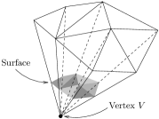
(b) A vertex linking surface

Figure 1. Normal surfaces within a triangulation

The concept of 0-efficiency is defined as follows [16]. If $\mathcal{T}$ is a closed or ideal triangulation, then we call $\mathcal{T}$ 0-efficient if and only if it contains no non-trivial normal spheres. If $\mathcal{T}$ is a bounded triangulation, then we call $\mathcal{T}$ 0-efficient if and only if it contains no non-trivial normal discs.

Jaco and Rubinstein describe a general “destructive” crushing procedure which they use for many purposes, such as creating 0-efficient triangulations of manifolds, and decomposing orientable manifolds into connected sums. This procedure is the main focus of this paper, and we describe it now in detail.

Definition 1.

Let $S$ be a normal surface in some generalised triangulation $\mathcal{T}$. The Jaco-Rubinstein crushing procedure operates on $S$ as follows:

1. We cut $\mathcal{T}$ open along the normal surface $S$. This converts the triangulation into a cell decomposition with a large variety of possible cell types (such as truncated tetrahedra, triangular or quadrilateral prisms, and truncated triangular prisms, some of which are illustrated in Figure 2). If $S$ is two-sided in $\mathcal{T}$ then we obtain two new copies of $S$ on the boundary of this cell decomposition, and if $S$ is one-sided in $\mathcal{T}$ then we obtain one new copy of the double cover of $S$ on the boundary.

   

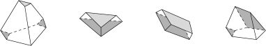
   Figure 2. Examples of cells obtained after cutting open along $S$

   

   Figure 3. Collapsing copies of $S$ on the boundary to points

2. We then collapse (or “shrink”) each copy of $S$ on the boundary to a point (using the quotient topology), as illustrated in Figure 3. Specifically, if $S$ was two-sided in $\mathcal{T}$ then we collapse the two copies of $S$ on the boundary to two points, and if $S$ was one-sided in $\mathcal{T}$ then we collapse the double cover of $S$ on the boundary to one point. This converts the triangulation into a cell decomposition $\mathcal{C}$, with cells of the following types:

   • 3-sided footballs, illustrated in Figure 4(a), which we obtain from regions of $\mathcal{T}$ between two parallel triangles of $S$, or between a triangle of $S$ and a tetrahedron vertex;

   • 4-sided footballs, illustrated in Figure 4(b), which we obtain from regions of $\mathcal{T}$ between two parallel quadrilaterals of $S$;

   • triangular purses, illustrated in Figure 4(c), which we obtain from regions of $\mathcal{T}$ between a quadrilateral of $S$ and nearby triangles or tetrahedron vertices;

   • tetrahedra, which we obtain from the central regions of tetrahedra in $\mathcal{T}$ that do not contain any quadrilaterals of $S$.

   

   (a) A 3-sided football

   

   (b) A 4-sided football

   

   (c) A triangular purse

   Figure 4. Destructively flattening non-tetrahedron cells

3. We next eliminate any non-tetrahedron cells, as illustrated in Figure 4, by simultaneously flattening all footballs to edges, and flattening all triangular purses to triangular faces (again using the quotient topology). Note that all remaining tetrahedron cells are preserved in this step (the flattening operations only affect cells with bigon faces).

   We can now “read off” a resulting generalised triangulation $\mathcal{T}_{\mathrm{JR}}$, which is defined only by the surviving tetrahedra and the resulting identifications between their 2-dimensional faces. In particular:

   • Any triangles, edges and/or vertices that do not belong to a tetrahedron are removed entirely, as illustrated in Figure 5(a). We might even lose entire connected components in this way.

   • If different pieces of a triangulation are connected along pinched edges or vertices then these pieces will “fall apart”, as illustrated in Figure 5(b) (since there are no 2-dimensional faces holding them together).

(a) Edges or faces not in a tetrahedron will disappear

(b) Tetrahedra joined along pinched edges or vertices will fall apart

Figure 5. Triangulations are defined by face gluings only

The final result of the crushing procedure is this generalised triangulation $\mathcal{T}_{\mathrm{JR}}$. Note that this might be disconnected, empty or invalid, and might not even represent a 3-manifold.

For convenience, we refer to steps 1 and 2 as non-destructive crushing (yielding the cell complex $\mathcal{C}$), and all three steps 1–3 as destructive crushing (yielding the generalised triangulation $\mathcal{T}_{\mathrm{JR}}$). Unless otherwise specified, “crushing” always refers to the full destructive operation.

We observe that each original tetrahedron $\Delta$ of $\mathcal{T}$ can only give rise to at most one tetrahedron of $\mathcal{T}_{\mathrm{JR}}$ (and only if $\Delta$ contains no quadrilaterals of $S$). It follows that $\mathcal{T}_{\mathrm{JR}}$ has strictly fewer tetrahedra than $\mathcal{T}$, unless $S$ is a union of vertex linking surfaces, in which case $\mathcal{T}_{\mathrm{JR}}$ and $\mathcal{T}$ are isomorphic (i.e., the crushing procedure has no effect).

Note that the intermediate cell decomposition $\mathcal{C}$ and the final triangulation $\mathcal{T}_{\mathrm{JR}}$ are well-defined. In particular, the flattening operations above can never result in any 2-face of a cell being identified with more than one partner 2-face, and the final triangulation $\mathcal{T}_{\mathrm{JR}}$ is independent of any “order” in which we flatten the footballs and/or purses of $\mathcal{C}$.

A key property of this procedure (which we generalise in Corollary 5) is that, for orientable manifolds, any “destructive” changes are both limited and detectable:

Theorem 2 (Jaco and Rubinstein [16]).

Let $\mathcal{T}$ be a generalised triangulation of a compact orientable 3-manifold $\mathcal{M}$ (with or without boundary), and let $S$ be a normal sphere or disc in $\mathcal{T}$. Then, if we destructively crush $S$ using the Jaco-Rubinstein procedure, we obtain a valid generalised triangulation $\mathcal{T}_{\mathrm{JR}}$ whose underlying 3-manifold $\mathcal{M}_{\mathrm{JR}}$ is obtained from $\mathcal{M}$ by zero or more of the following operations:

• undoing connected sums, i.e., replacing some intermediate manifold $\mathcal{M}^{\prime}$ with the disjoint union $\mathcal{M}^{\prime}_{1}\cup\mathcal{M}^{\prime}_{2}$, where $\mathcal{M}^{\prime}=\mathcal{M}^{\prime}_{1}\ \#\ \mathcal{M}^{\prime}_{2}$;

• cutting open along properly embedded discs;

• filling boundary spheres with 3-balls;

• deleting 3-ball, 3-sphere, $\mathbb{R}P^{3}$, $L_{3,1}$ or $S^{2}\times S^{1}$ components.

For reference, Jaco and Rubinstein do not present Theorem 2 in this unified form—the theorem statement above collects the results of several detailed arguments from throughout their original paper [16].

We emphasise again that all generalised triangulations and cell decompositions in this paper are defined entirely by their 3-cells and the pairwise identifications between the 2-faces of these 3-cells. In particular, if we modify a cell decomposition so that some edge or 2-face does not belong to a 3-cell then that edge or 2-face will disappear (as in Figure 5(a)), and if different pieces of the cell decomposition become connected along pinched edges or vertices then those pieces will fall apart (as in Figure 5(b)).

2. The crushing lemma

In this section we present our “atomic” formulation of the Jaco-Rubinstein crushing procedure. We begin with the crushing lemma (Lemma 3), which establishes the sufficiency of our three atomic operations, and shows that they can be performed sequentially (as opposed to simultaneously). Lemma 4 then analyses the precise behaviour of each operation on a compact manifold, and Corollary 5 uses this to prove a generalisation of Theorem 2 that covers both orientable and non-orientable manifolds.

We emphasise that the crushing lemma is completely general: the triangulation may be non-orientable, or ideal, or even invalid. In this sense, the crushing lemma is intended as a launching point for generalising crushing and 0-efficiency technology to a wide range of settings (such as ideal triangulations, which we do not pursue in detail in this short paper).

The proof of the crushing lemma uses an algorithmic approach: we show how the full crushing procedure can be performed one atomic operation at a time. We note that this algorithm is intended to assist with the theoretical analysis, not the implementation; a practical implementation could simply flatten non-tetrahedron cells “in bulk”.

Lemma 3 (Crushing lemma).

Let $\mathcal{T}$ be a generalised triangulation containing a normal surface $S$. Let $\mathcal{C}$ be the cell decomposition obtained by non-destructively crushing $S$, as described in steps (1)–(2) of Definition 1, and let $\mathcal{T}_{\mathrm{JR}}$ be the final triangulation obtained at the end of the destructive crushing procedure, after flattening away all non-tetrahedron cells in step (3) of Definition 1. Then $\mathcal{T}_{\mathrm{JR}}$ can be obtained from $\mathcal{C}$ by a sequence of zero or more of the following atomic operations, one at a time, in some order:

• flattening a triangular pillow to a triangular face, as shown in Figure 6(a);

• flattening a bigonal pillow to a bigon face, as shown in Figure 6(b);

• flattening a bigon face to an edge, as shown in Figure 6(c).

As in Definition 1, after each atomic operation we remove any “orphaned” 2-faces, edges or vertices that do not belong to a 3-cell, and we pull apart any pieces of the cell decomposition that are connected along pinched edges or vertices (as in Figure 5).

(a) Flattening a triangular pillow

(b) Flattening a bigonal pillow

(c) Flattening a bigon face

Figure 6. Atomic moves for the Jaco-Rubinstein crushing procedure

Note that each atomic operation might be performed several times, and that multiple instances of one operation might be interspersed with instances of the others.

Proof.

Recall that in the cell decomposition $\mathcal{C}$, there are only three types of cells that are not tetrahedra: 3-sided footballs, 4-sided footballs and triangular purses, which $\mathcal{T}_{\mathrm{JR}}$ flattens to edges, edges and triangles respectively. In addition to these, we now describe three intermediate cell types which might appear as we incrementally convert $\mathcal{C}$ into $\mathcal{T}_{\mathrm{JR}}$:

• triangular pillows, as seen earlier in Figure 6(a);

• bigonal pillows, as seen earlier in Figure 6(b);

• bigonal pyramids, a new cell type shown in Figure 7(d), which $\mathcal{T}_{\mathrm{JR}}$ flattens to a triangle.

For reference, all six original and intermediate cell types are illustrated in Figure 7.

(a) A 3-sided football

(b) A 4-sided football

(c) A triangular purse

(d) A bigonal pyramid

(e) A triangular pillow

(f) A bigonal pillow

Figure 7. All six original and intermediate cell types

The crushing process requires us to simultaneously flatten footballs to edges and purses to triangles; our task now is to find a good order in which to do this, so that we obtain a sequence of atomic operations as described above. The key complication is that local moves on one cell might change the shapes of adjacent cells, and so we must choose our ordering carefully to avoid creating any unexpected new cell types.

Our solution is to convert $\mathcal{C}$ into $\mathcal{T}_{\mathrm{JR}}$ by applying the following algorithm:

1. If there are any triangular pillows, flatten them to triangles.

2. If there are any bigonal pillows, flatten them to bigons.

3. If there is a 3-sided football, then choose one of its bigon faces which is not identified with another face of the same 3-cell, flatten this bigon to an edge (which will also change the shape of the adjacent cell, if there is one), and return to step (1).

4. If there is a 4-sided football, then choose any one of its bigon faces, flatten this bigon to an edge, and return to step (1).

5. If there are any bigonal pyramids or triangular purses, flatten all of their bigon faces to edges and return to step (1).

We first note that the choice in step (3) is always possible because a 3-sided football has an odd number of bigon faces. Moreover, the various flattening operations never introduce any new cell types beyond the six listed above:

• In steps (3) and (4), the 3-sided football becomes a bigonal pillow, and the 4-sided football becomes either a bigonal pillow or a 3-sided football according to whether the chosen bigon joins the football with itself or a different cell. The adjacent cell (if there is one) changes as follows: Because we have already eliminated bigonal pillows, the adjacent cell must be a 3-sided football, a 4-sided football, a triangular purse, or a bigonal pyramid. Flattening the bigon then converts this to a bigonal pillow, a 3-sided football, a bigonal pyramid, or a triangular pillow respectively.

• In step (5), the only non-tetrahedron cell types remaining are triangular pillows with one or two bigon sides, and so flattening bigons converts all of these cells to triangular pillows.

We run the algorithm above until there are no remaining non-tetrahedron cells. The algorithm terminates because in each iteration it strictly reduces the number of non-tetrahedron cells plus the number of bigons. The resulting triangulation is then $\mathcal{T}_{\mathrm{JR}}$, and the only atomic operations that the algorithm performs are flattening triangular pillows, bigonal pillows and bigons, one at a time. ∎

One might observe that the crushing lemma simply replaces the three original moves of Figure 4 with the three atomic moves of Figure 6. Nevertheless, this brings important advantages:

• The new atomic moves operate on smaller subcomplexes (triangular pillows, bigonal pillows and bigon faces), which means fewer special cases or unusual behaviours to analyse.

• More importantly, our new atomic moves can be performed sequentially, and can therefore be studied individually as local operations. The original flattening moves of Figure 4 must be done simultaneously (otherwise we introduce many additional cell types each with their own moves and analyses), which means the original flattening moves must be studied as a complex global operation (as Jaco and Rubinstein do in their original paper).

• We extend our analysis to more general settings, such as non-orientable triangulations and arbitrary ideal triangulations.

From this point onwards we restrict our attention to compact manifolds (i.e., closed or bounded triangulations), and study the possible outcomes of each of our three atomic moves.

Lemma 4.

Let $\mathcal{C}$ be a cell decomposition of a compact 3-manifold $\mathcal{M}$ (with or without boundary) that contains no two-sided projective planes. Then applying one of the atomic moves of Lemma 3 will yield a (valid) cell decomposition of a 3-manifold $\mathcal{M}^{\prime}$, where either $\mathcal{M}^{\prime}=\mathcal{M}$, or else $\mathcal{M}^{\prime}$ is obtained from $\mathcal{M}$ by one of the following operations:

• If we flattened a triangular pillow, then $\mathcal{M}^{\prime}$ might remove a single connected 3-ball, 3-sphere or $L_{3,1}$ component from $\mathcal{M}$;

• If we flattened a bigonal pillow, then $\mathcal{M}^{\prime}$ might remove a single connected 3-ball, 3-sphere or $\mathbb{R}P^{3}$ component from $\mathcal{M}$;

• If we flattened a bigon face, then (i) $\mathcal{M}^{\prime}$ might be obtained by cutting $\mathcal{M}$ open along a properly embedded disc, (ii) $\mathcal{M}^{\prime}$ might be obtained by filling one boundary sphere of $\mathcal{M}$ with a 3-ball; (iii) $\mathcal{M}^{\prime}$ might be obtained by cutting $\mathcal{M}$ open along an embedded sphere and filling the two resulting boundary spheres with 3-balls; or (iv) we might have $\mathcal{M}=\mathcal{M}^{\prime}\ \#\ \mathbb{R}P^{3}$; that is, $\mathcal{M}^{\prime}$ might remove a single $\mathbb{R}P^{3}$ summand from the connected sum decomposition of $\mathcal{M}$.

Proof.

The pillow moves are easiest to handle. Because they do not affect the 1-skeleton of $\mathcal{C}$, it is clear that the resulting cell decomposition remains valid. Let $F_{1},F_{2}$ be the two faces bounding the (triangular or bigonal) pillow.

• If $F_{1}$ and $F_{2}$ both lie in the boundary of the manifold then the pillow is an entire 3-ball component, and flattening the pillow simply deletes this component.

• If $F_{1}$ and $F_{2}$ are identified together then the pillow is a single connected component of one of the following topological types:

  • $L_{3,1}$ (obtained by identifying the faces of a triangular pillow with a twist);

  • $\mathbb{R}P^{3}$ (obtained by identifying the faces of a bigon pillow with a twist);

  • $S^{3}$ (obtained by identifying the faces of a triangular or bigon pillow without a twist).

  Here we ignore orientation-reversing identifications between $F_{1}$ and $F_{2}$, because these imply that $\mathcal{C}$ has either an edge identified with itself in reverse (i.e., an invalid cell decomposition) or a non-orientable vertex link.

• Otherwise, $F_{1}$ and $F_{2}$ are not identified (so their relative interiors are disjoint) and they are not both boundary, whereby flattening them together does not change the underlying 3-manifold.

Flattening a bigon face to an edge is a little more delicate, with several cases to consider. Let $e_{1},e_{2}$ be the two edges bounding the bigon.

• If the entire bigon lies in the boundary of the manifold:

  • If $e_{1}$ and $e_{2}$ are not identified (so their relative interiors are disjoint), then flattening them together does not change the underlying 3-manifold.

  • If $e_{1}$ and $e_{2}$ are identified then (since $\mathcal{M}$ contains no two-sided projective planes) this must be as a sphere. Flattening the bigon then has the effect of filling this boundary sphere with a 3-ball, as illustrated in Figure 8.

  

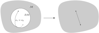
  Figure 8. Flattening a bigon that forms a sphere on the boundary

• If the bigon does not lie in the boundary and $e_{1}$ and $e_{2}$ are identified together so that the bigon forms a sphere, then flattening the bigon has the effect of slicing $\mathcal{M}$ open along this sphere and filling the resulting boundary spheres with 3-balls, as illustrated in Figure 9. Note that this is true even if the edges and/or vertices of the bigon do lie in the boundary, as illustrated in Figure 10.

  

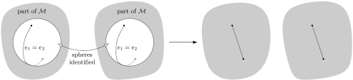
  Figure 9. Flattening a bigon that forms an internal sphere

  

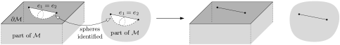
  Figure 10. Flattening a bigon that forms a sphere touching the boundary

• If the bigon does not lie in the boundary and $e_{1}$ and $e_{2}$ are identified together so that the bigon forms a projective plane, then (by our initial assumptions) this must be a one-sided projective plane $P$. We can view the move in two stages: (i) unglue the two cells on either side of the bigon (since this gluing will be lost after the move anyway), which yields two boundary bigons; and then (ii) flatten these two boundary bigons to edges.

  If the entire bigon is internal to the manifold then, topologically, stage (i) cuts along a sphere surrounding $P$ and discards the connected component containing $P$, and then stage (ii) fills the remaining sphere boundary with a 3-ball. That is, we remove a single $\mathbb{R}P^{3}$ summand from the connected sum decomposition of $\mathcal{M}$.

  If the edge and/or vertex of this bigon lies in the boundary of $\mathcal{M}$ then stage (i) may introduce temporary anomalies (such as punctures in vertex linking discs), but stage (ii) fixes these so that, like the sphere case before, the full move has the same net topological effect regardless of whether the bigon is internal.

  Note that this operation does not create an invalid edge, even though the original edges $e_{1},e_{2}$ that surround the bigon are identified in reverse. This is because the projective plane is one-sided, and so stage (i) creates a single sphere boundary formed from two bigons (the double cover of the original projective plane), which then allows us to flatten both boundary bigons without problems. If the projective plane were two-sided then we would indeed create two invalid edges; we return to this possibility in Lemma 6.

• If the bigon does not lie in the boundary, and $e_{1}$ and $e_{2}$ are not identified but both $e_{1}$ and $e_{2}$ do lie in the boundary, then flattening the bigon has the effect of slicing $\mathcal{M}$ open along the corresponding disc, as illustrated in Figure 11.

  

  Figure 11. Flattening a bigon whose edges encircle the boundary

• Otherwise $e_{1}$ and $e_{2}$ are not identified (so their relative interiors are disjoint) and not both boundary, and so flattening them together does not change the underlying 3-manifold. ∎

Now that we understand the possible behaviour of each atomic move, we can aggregate this information to understand the Jaco-Rubinstein crushing procedure as a whole. In the following result we do this for arbitrary compact manifolds, thereby generalising Theorem 2 to both orientable and non-orientable settings. As in the previous lemma, we exclude two-sided projective planes (which can lead to invalid edges); however, even this exclusion can be partially overcome as we see later in Section 3.

Corollary 5.

Let $\mathcal{T}$ be a generalised triangulation of a compact 3-manifold $\mathcal{M}$ (with or without boundary) that contains no two-sided projective planes, and let $S$ be a normal sphere or disc in $\mathcal{T}$. Then, if we destructively crush $S$ using the Jaco-Rubinstein procedure, we obtain a valid triangulation $\mathcal{T}_{\mathrm{JR}}$ whose underlying 3-manifold $\mathcal{M}_{\mathrm{JR}}$ is obtained from $\mathcal{M}$ by zero or more of the following operations:

• undoing connected sums, i.e., replacing some intermediate manifold $\mathcal{M}^{\prime}$ with the disjoint union $\mathcal{M}^{\prime}_{1}\cup\mathcal{M}^{\prime}_{2}$, where $\mathcal{M}^{\prime}=\mathcal{M}^{\prime}_{1}\ \#\ \mathcal{M}^{\prime}_{2}$;

• cutting open along properly embedded discs;

• filling boundary spheres with 3-balls;

• deleting 3-ball, 3-sphere, $\mathbb{R}P^{3}$, $L_{3,1}$, $S^{2}\times S^{1}$ or twisted $S^{2}\stackrel{{\scriptstyle\smash{\raisebox{-2.84526pt}[0.0pt][0.0pt]{$\scriptstyle\sim$}}}}{{\times}}S^{1}$ components.

Proof.

This follows immediately from Lemmata 3 and 4, and the fact that the non-destructive act of crushing $S$ to a point (which precedes the sequence of atomic moves) has the effect of either undoing a connected sum (if $S$ is a separating sphere), removing an $S^{2}\times S^{1}$ or twisted $S^{2}\stackrel{{\scriptstyle\smash{\raisebox{-2.84526pt}[0.0pt][0.0pt]{$\scriptstyle\sim$}}}}{{\times}}S^{1}$ summand from the connected sum decomposition (if $S$ is a non-separating sphere), or cutting along a properly embedded disc (if $S$ is a disc). ∎

3. Non-orientable prime decomposition

We now give an application of our earlier results: a modern approach to prime decomposition of non-orientable manifolds based on the crushing process.

In 1995, Jaco and Tollefson described an algorithm that, given a closed 3-manifold triangulation $\mathcal{T}$, decomposes the underlying manifold into a connected sum of prime manifolds [18]. In essence, it involves the following steps:

1. Enumerate all vertex normal spheres in $\mathcal{T}$. These are normal spheres that are represented by extreme rays of a high-dimensional polyhedral cone derived from the triangulation $\mathcal{T}$; see [18] for a precise definition.

2. Convert these into a (possibly much larger) collection of pairwise disjoint embedded spheres in $\mathcal{T}$ using an intricate series of cut-and-paste operations.

3. Cut $\mathcal{T}$ open along these embedded spheres, retriangulate, and fill the boundaries with balls to obtain the final list of irreducible summands.

Despite its theoretical importance, the Jaco-Tollefson algorithm is both slow and complex. Step 1 requires us to enumerate all vertex normal spheres (of which there could be exponentially many), which prevents us from using highly effective optimisations based on linear programming [8]. Step 2 is extremely complex to implement, and could significantly increase the number of spheres under consideration (which is already exponential in the number of tetrahedra). Likewise, the cut-open-and-retriangulate operation of step 3 is highly intricate to implement, and could vastly increase the number of tetrahedra in the final collection of triangulated summands.

For orientable triangulations, the Jaco-Rubinstein theory of 0-efficiency from 2003 simplified this algorithm enormously [16]. In brief, the new procedure is:

1. Locate any non-trivial normal sphere in the triangulation, and destructively crush this to obtain a new (possibly disconnected) triangulation with strictly fewer tetrahedra. Repeat this step for as long as a non-trivial normal sphere can be found.

2. Once no non-trivial normal spheres exist (i.e., the remaining triangulation is 0-efficient), each connected component of the triangulation represents a single prime summand. There may be additional “missing” summands that were lost, but these can be reconstructed by tracking changes in homology.

This 0-efficiency-based algorithm is much faster (though still exponential time), and is significantly cleaner to implement. Moreover, it becomes far simpler to detect and discard trivial 3-sphere summands, since 3-sphere recognition is significantly less demanding for 0-efficient triangulations than for general inputs [16]. Historically this algorithm was the turning point at which prime decomposition first became practical, and in 2004 it became the foundation for the first real software implementation [3].

For non-orientable triangulations, the state of the art remains the original Jaco-Tollefson algorithm, which has still never been implemented due to the speed and intricacy reasons outlined above. Here we now use the results of Section 2 to develop a fast and simple prime decomposition algorithm for non-orientable triangulations, based on 0-efficiency and the Jaco-Rubinstein crushing process.

In this setting there is a major complication: for non-orientable manifolds, the Jaco-Rubinstein crushing process might leave us with an invalid triangulation, where some edge is identified with itself in reverse. As noted in the detailed proof of Lemma 4, this can only occur if the triangulation contains an embedded two-sided projective plane.

We employ a “permissive” strategy for dealing with this complication: we run the algorithm regardless of whether there might be problems, and after it finishes we test whether anything went wrong by looking for invalid edges (an easy test to perform). This permissive approach has two benefits:

• There are no onerous preconditions to test before we run the algorithm. Instead we can start the algorithm immediately, oblivious to whether there is an embedded two-sided projective plane or not.

• The algorithm might still succeed even if there is an embedded two-sided projective plane: if we “get lucky” and do not create an invalid edge, we still guarantee correctness. If we are unlucky and we do create an invalid edge during some atomic move, we prove that this can be detected after the fact, once the crushing process is complete.

We begin this section with Lemma 6, a non-orientable extension to Corollary 5 that uses the crushing lemma to identify the possible consequences of crushing in the presence of two-sided projective planes. In the proof we take care to ensure that, if an atomic move ever creates an invalid edge, then any subsequent atomic moves preserve the existence of invalid edges. We follow this with the full prime decomposition algorithm, as detailed in Algorithm 7.

Lemma 6.

Let $\mathcal{T}$ be a generalised triangulation of any closed compact 3-manifold $\mathcal{M}$, and let $S$ be a normal sphere in $\mathcal{T}$. Then, if we destructively crush $S$ using the Jaco-Rubinstein procedure, one of the following things happens:

1. we obtain an invalid triangulation, in which some edge is identified with itself in reverse;

2. we obtain a valid triangulation $\mathcal{T}_{\mathrm{JR}}$ whose underlying 3-manifold $\mathcal{M}_{\mathrm{JR}}$ is obtained from $\mathcal{M}$ by zero or more of the following operations:

   • undoing connected sums, i.e., replacing some intermediate manifold $\mathcal{M}^{\prime}$ with the disjoint union $\mathcal{M}^{\prime}_{1}\cup\mathcal{M}^{\prime}_{2}$, where $\mathcal{M}^{\prime}=\mathcal{M}^{\prime}_{1}\ \#\ \mathcal{M}^{\prime}_{2}$;

   • deleting 3-sphere, $\mathbb{R}P^{3}$, $L_{3,1}$, $S^{2}\times S^{1}$ or twisted $S^{2}\stackrel{{\scriptstyle\smash{\raisebox{-2.84526pt}[0.0pt][0.0pt]{$\scriptstyle\sim$}}}}{{\times}}S^{1}$ components.

Moreover, (1) can only occur if $\mathcal{M}$ contains an embedded two-sided projective plane.

Proof.

If $\mathcal{M}$ does not contain an embedded two-sided projective plane then this is a special case of Corollary 5 (restricted to closed manifolds), and it is immediate that we obtain outcome (2) above.

If we do allow $\mathcal{M}$ to contain embedded two-sided projective planes, we must examine how this affects our three atomic operations from Lemma 3: flattening triangular pillows, flattening bigonal pillows, and flattening bigon faces. In essence, we find that things behave well around the vertices, but we may create invalid edges (edges identified with themselves in reverse). This occurs precisely when we flatten a bigon face whose edges are identified to form a two-sided projective plane; we describe this operation in more detail shortly. Note that both endpoints of any invalid edge $e$ must be identified; that is, $e$ is incident to one and only one vertex.

Before proceeding, we observe that every vertex link remains a 2-sphere under all three atomic operations. This is because (i) flattening a triangular or bigonal pillow removes an entire connected component, and so cannot introduce a non-spherical vertex link; and (ii) flattening a bigon face effectively collapses two curves to a point in the vertex links, which might split a 2-sphere link into multiple 2-spheres, but which cannot introduce new genus or orientation-reversing paths.

As we consider each atomic move, we show that either the move is consistent with outcome (2) above, or else we carefully study how it affects the number and location of any invalid edges. By the “location” of an invalid edge, we mean the incident vertex (of which there is only one, as noted above).

Our first step is to remove triangular pillows from consideration. Here we observe that nothing “goes wrong”, in that flattening a triangular pillow is always consistent with outcome (2) above, and never changes the number or location of any invalid edges. Let $F_{1},F_{2}$ be the two triangular faces bounding such a pillow:

• If $F_{1}$ and $F_{2}$ are not identified then flattening the pillow does not change the underlying 3-manifold, and although the pillow may be surrounded by one or more invalid edges, flattening the pillow does not change their number or location.

• If $F_{1}$ and $F_{2}$ are identified in an orientation-preserving fashion, then the pillow is a single $S^{3}$ or $L_{3,1}$ component (with no invalid edges), and flattening the pillow simply removes this component.

• If $F_{1}$ and $F_{2}$ are identified in an orientation-reversing fashion then one of the vertices of the pillow will have a non-orientable link, which we know from above can never occur.

We next “limit the damage” that can occur from bigonal pillows. Here we show that flattening a bigonal pillow is either consistent with outcome (2) above with no change in the number or location of invalid edges, or else it removes precisely two invalid edges, both of which are incident to the same vertex. Again, let $F_{1},F_{2}$ be the two bigon faces bounding such a pillow:

• If $F_{1}$ and $F_{2}$ are not identified then flattening the pillow does not change the underlying 3-manifold, and again does not affect the number or location of any invalid edges.

• If $F_{1}$ and $F_{2}$ are identified in an orientation-preserving fashion, then the pillow is a single $S^{3}$ or $\mathbb{R}P^{3}$ component (with no invalid edges), and as before flattening the pillow simply removes this component.

• Suppose that $F_{1}$ and $F_{2}$ are identified in an orientation-reversing fashion. There are two choices of identification: (i) one that maps each edge of the bigon to the other, and (ii) one that maps each edge to itself in reverse. The first option yields non-orientable vertex links, and so cannot occur. The second option yields precisely two invalid edges, both incident to the same vertex, and the flattening operation removes the entire pillow along with both of these invalid edges.

This leaves us with the most problematic move: flattening a bigon face. Let $e_{1},e_{2}$ be the two edges bounding such a face. Here one of several things can occur:

• If $e_{1}$ and $e_{2}$ are both valid edges, and if they are not identified in a way that makes the bigon form a two-sided projective plane, then things work exactly as in the proof of Lemma 4: we might slice $\mathcal{M}$ open along a sphere and fill the resulting boundaries with 3-balls, or we might remove a single $\mathbb{R}P^{2}$ summand from the connected sum decomposition of $\mathcal{M}$, or we might simply leave the manifold unchanged. All of these possibilities are consistent with outcome (2) above.

  Here we do not change the number of invalid edges, but we might change their locations. Specifically, we might split a vertex $V$ into multiple vertices $V_{1},V_{2}$ (e.g., when undoing a connected sum), whereupon the invalid edges that touched $V$ will become distributed amongst $V_{1}$ and $V_{2}$ in some manner. Note that we might even perform more than one such split.

  

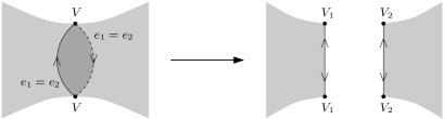
  Figure 12. Flattening a bigon that forms a two-sided projective plane

• If $e_{1}$ and $e_{2}$ are both valid edges, and if they are identified in a way that makes the bigon form a two-sided projective plane, then the move has the following effect. We cut the manifold open along this projective plane, and then flatten each of the two $\mathbb{R}P^{2}$ boundary components to a single invalid edge, as illustrated in Figure 12. Note that the midpoint of each invalid edge has a small regular neighbourhood bounded by $\mathbb{R}P^{2}$ (not $S^{2}$ as usual).

  The outcome is that we create two new invalid edges. The locations change as follows: the original vertex $V$ splits into two vertices $V_{1},V_{2}$; any previous invalid edges that touched $V$ become distributed amongst $V_{1}$ and $V_{2}$ in some manner; and then each of $V_{1}$ and $V_{2}$ acquires one of the new invalid edges that is created by the move.

• If one edge (say $e_{1}$) is valid but the other (say $e_{2}$) is invalid, then the move merges these together into a single invalid edge that is incident with the same vertex as the original $e_{2}$. That is, both the number and location of all invalid edges stays the same.

• If $e_{1}$ and $e_{2}$ are both invalid, then we note that they must both be incident to the same vertex. If $e_{1}$ and $e_{2}$ are invalid and not identified, then the move merges $e_{1}$ and $e_{2}$ together into a single valid edge (the orientation twists around $e_{1}$ and $e_{2}$ effectively cancel each other when the edges are merged). The result is that we lose precisely two invalid edges, both of which were incident to the same vertex.

• If $e_{1}$ and $e_{2}$ are both invalid, and if they are identified, then the bigon must form a sphere whose edge is identified with itself in reverse due to a twist on one side of the sphere, as illustrated in Figure 13. The move essentially (i) cuts the manifold open along this sphere, leaving an $\mathbb{R}P^{2}$ boundary on the side with the twist and a sphere boundary on the other side, and then (ii) flattens each of these boundaries to a single edge, creating an invalid edge on the $\mathbb{R}P^{2}$ side. The full move is illustrated in Figure 13.

  The outcome is that the total number of invalid edges is preserved (including our original edge $e_{1}=e_{2}$, which becomes the flattened $\mathbb{R}P^{2}$ boundary). Regarding locations: again the original vertex $V$ splits into multiple vertices $V_{1},V_{2},V_{3}$, whereupon the invalid edges originally incident to $V$ become distributed amongst $V_{1},V_{2},V_{3}$ in some manner.

  

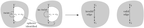
  Figure 13. Flattening a bigon that joins an invalid edge to itself

In summary: taking into account all three atomic moves, we find that if no invalid edges are ever created, then we obtain outcome (2) from the lemma statement. Our final goal is to show that, if invalid edges are ever created, that at least one of them survives to the end of the crushing procedure; that is, we obtain outcome (1).

This is now just a matter of parity. Define an odd or even vertex to be one that is incident with an odd or even number of invalid edges respectively. The first time we create a pair of invalid edges, these are incident with different vertices; that is, we create two odd vertices. It is now simple to see that none of the moves can ever reduce the number of odd vertices:

• whenever we split a vertex $V$ and redistribute its incident edges amongst the resulting vertices $V_{1},V_{2},\ldots$, if the original vertex $V$ was odd then one of the resulting vertices $V_{i}$ must be odd also;

• if we ever create a new pair of invalid edges from a two-sided projective plane incident to some original odd vertex $V$, then the two resulting vertices $V_{1}$ and $V_{2}$ must have different parities, and so one of these must be odd also;

• whenever we lose a pair of invalid edges (either through flattening a bigon or flattening a bigonal pillow), these invalid edges are always incident to the same vertex and so parities are preserved.

It follows that, if we ever create an invalid edge at any stage, then we will have odd vertices remaining at the end of the crushing process; that is, we will have invalid edges as described in outcome (1). ∎

We can now package the results of Lemma 6 into a general algorithm for computing the prime decomposition of a triangulated 3-manifold, either orientable or non-orientable. The structure of the algorithm follows the modern “ready to implement” framework presented in [5] for the orientable case. The process can be further improved by simplifying triangulations at key stages of the algorithm; we omit this here, but details can be found in [5].

Algorithm 7 (Prime decomposition).

Given an input triangulation $\mathcal{T}$ of any closed connected 3-manifold $\mathcal{M}$, the following algorithm will either decompose $\mathcal{M}$ into a connected sum of prime manifolds, or else prove that $\mathcal{M}$ contains an embedded two-sided projective plane.

1. Compute the first homology of $\mathcal{T}$, and let $r$, $t_{2}$ and $t_{3}$ denote the $\mathbb{Z}$ rank, $\mathbb{Z}_{2}$ rank and $\mathbb{Z}_{3}$ rank respectively.

2. Create an input list $\mathcal{L}$ of triangulations to process, initially containing just $\mathcal{T}$, and an output list $\mathcal{O}$ of prime summands, initially empty.
   While $\mathcal{L}$ is non-empty:

   • Let $\mathcal{N}$ be the next triangulation in the list $\mathcal{L}$. Remove $\mathcal{N}$ from $\mathcal{L}$, and test whether $\mathcal{N}$ has a non-trivial normal sphere $F$.

     • If there is such a normal sphere, then perform the Jaco-Rubinstein crushing procedure on $F$.

       • If the resulting triangulation has an invalid edge, then terminate with the statement that the input manifold contains an embedded two-sided projective plane.

       • If the resulting triangulation has no invalid edges, then add each connected component of the resulting triangulation back into the list $\mathcal{L}$.

     • If there is no such normal sphere, then append $\mathcal{N}$ to the output list $\mathcal{O}$.

3. Compute the first homology of each triangulation in the output list $\mathcal{O}$, and let $r^{\prime}$, $t_{2}^{\prime}$ and $t_{3}^{\prime}$ denote the sums of the $\mathbb{Z}$ ranks, $\mathbb{Z}_{2}$ ranks and $\mathbb{Z}_{3}$ ranks respectively.

4. Append $(t_{2}-t_{2}^{\prime})$ copies of $\mathbb{R}P^{3}$ and $(t_{3}-t_{3}^{\prime})$ copies of $L_{3,1}$ to $\mathcal{O}$. If the input triangulation was orientable, append $(r-r^{\prime})$ copies of $S^{2}\times S^{1}$ to $\mathcal{O}$, and otherwise append $(r-r^{\prime})$ copies of the twisted product $S^{2}\stackrel{{\scriptstyle\smash{\raisebox{-2.84526pt}[0.0pt][0.0pt]{$\scriptstyle\sim$}}}}{{\times}}S^{1}$ to $\mathcal{O}$.

If we did not terminate earlier due to an invalid edge, then the final output list $\mathcal{O}$ will contain a collection of triangulated prime manifolds $\mathcal{O}_{1},\ldots,\mathcal{O}_{k}$ for which the original manifold $\mathcal{M}$ can be expressed as the connected sum $\mathcal{O}_{1}\#\mathcal{O}_{2}\#\ldots\#\mathcal{O}_{k}$.

The correctness of this algorithm follows immediately from Lemma 6 (the changes in $\mathbb{Z}$, $\mathbb{Z}_{2}$ and $\mathbb{Z}_{3}$ ranks indicate the number of $S^{2}\times S^{1}$ or $S^{2}\stackrel{{\scriptstyle\smash{\raisebox{-2.84526pt}[0.0pt][0.0pt]{$\scriptstyle\sim$}}}}{{\times}}S^{1}$, $\mathbb{R}P^{3}$, and $L_{3,1}$ summands that were lost respectively). If the input triangulation contains $n$ tetrahedra, it is clear that we terminate after crushing at most $n$ normal spheres, since each crushing operation strictly reduces the total number of tetrahedra in the input list $\mathcal{L}$. Note that some of the output manifolds $\mathcal{O}_{k}$ might be trivial (i.e., redundant 3-sphere summands); however, such trivial summands are easy to detect, as outlined below.

As presented above, this algorithm gives the summands in the connected sum decomposition, but these may not uniquely define the original manifold (since there can be orientation-related decisions to make when performing the connected sum operation). This can be resolved by tracking orientations explicitly through the crushing process, a straightforward but slightly messy enhancement to the algorithm that we do not describe in detail here.

We finish this section with some implementation notes:

• There are well-known polynomial-time procedures for computing homology in step (1), based on Smith normal form; see [10, 11] for examples.

• In step (• ‣ 2) we must locate a non-trivial normal sphere, if one exists. Traditionally, one does this by enumerating all quadrilateral vertex normal surfaces; see [5] for details on what this means and why it works. A newer (and experimentally much faster) alternative is to make a targeted search for a normal sphere using branch-and-bound techniques from combinatorial optimisation; see [8] for details.

• It is easy to eliminate trivial 3-sphere summands from the output list. If an output triangulation $\mathcal{O}_{i}$ has non-trivial homology then it is a non-trivial summand; otherwise $\mathcal{O}_{i}$ must be 0-efficient, whereupon Jaco and Rubinstein show that $\mathcal{O}_{i}$ is trivial if and only if (i) it has more than one vertex, or (ii) it contains an embedded almost normal sphere. See [16] for details on almost normal spheres, and see [4, 8] for fast algorithms for detecting them.

4. Minimal triangulations

Our final application uses crushing techniques to study the combinatorics of minimal triangulations of both orientable and non-orientable manifolds. A minimal triangulation of a 3-manifold $\mathcal{M}$ is one that triangulates $\mathcal{M}$ using the fewest possible tetrahedra. Minimal triangulations are the focus of many censuses of low-complexity 3-manifolds [22]; in such censuses it is common to focus on $\mathbb{P}^{2}$-irreducible 3-manifolds, in which every embedded 2-sphere bounds a 3-ball, and in which there are no embedded two-sided projective planes.

There are many simple combinatorial properties that a minimal triangulation of a closed $\mathbb{P}^{2}$-irreducible manifold must satisfy (for instance, with a few exceptions it must have just one vertex, and no low-degree edges). Often these properties are proven using ad-hoc constructions that show how, if a property is not satisfied, then the triangulation can be simplified to use fewer tetrahedra.

As part of their study on 0-efficient triangulations [16], Jaco and Rubinstein prove several of these properties for orientable manifolds using 0-efficiency techniques. Although these are in most cases rederivations of known results, their proofs essentially unify these results: instead of a collection of ad-hoc constructions, they show how these results all follow immediately from the observation that (modulo a few exceptions) a minimal triangulation must be 0-efficient.

Here we extend these arguments to the non-orientable setting. Again most of the results we prove are already known; the purpose of this section is to unify them as immediate consequences of 0-efficiency. Much of this section follows Jaco and Rubinstein directly, and so we keep the exposition brief and only present details where the arguments diverge.

All of the results in this section rely on the following core observation, which Jaco and Rubinstein prove for orientable manifolds [16], and which we prove here in the general case.

Theorem 8.

Let $\mathcal{M}$ be a closed $\mathbb{P}^{2}$-irreducible 3-manifold (which may be orientable or non-orientable) that is not $\mathbb{R}P^{3}$ or $L_{3,1}$. Then every minimal triangulation of $\mathcal{M}$ is 0-efficient.

Proof.

This follows immediately from Corollary 5: if a triangulation of $\mathcal{M}$ is not 0-efficient, then performing the Jaco-Rubinstein crushing procedure on a normal 2-sphere will produce a new triangulation of $\mathcal{M}$ with fewer tetrahedra.

If $\mathcal{M}$ is the 3-sphere then crushing might remove $\mathcal{M}$ entirely, but in this case we simply note that both minimal triangulations of $S^{3}$ (each with one tetrahedron) are 0-efficient, as observed earlier in [16]. ∎

We now turn to proving various properties of minimal triangulations. Our first result—that a minimal triangulation must have one vertex—was originally proven by Matveev for orientable manifolds [23] and Martelli and Petronio in the general case [21], both working in the dual setting of special spines. Jaco and Rubinstein rederive this for orientable manifolds as a simple corollary of 0-efficiency [16], and here we observe that their argument translates directly to the non-orientable case.

Corollary 9.

Let $\mathcal{T}$ be a minimal triangulation of a closed $\mathbb{P}^{2}$-irreducible 3-manifold (which may be orientable or non-orientable) that is not $S^{3}$, $\mathbb{R}P^{3}$ or $L_{3,1}$. Then $\mathcal{T}$ contains precisely one vertex.

Proof.

We first show that any 0-efficient triangulation with $\geq 2$ vertices must represent the 3-sphere. This is a direct copy of Jaco and Rubinstein’s barrier surface argument from [16, Proposition 5.1], and we do not repeat it here. The essential details are as follows.

If $\mathcal{T}$ has two distinct vertices, then it has some edge $e$ that joins them. Place a sphere $S$ around $e$, and attempt to normalise $S$. Since the edge $e$ acts as a barrier to normalisation, and since the triangulation is 0-efficient, $S$ must normalise to a (possibly empty) union of vertex linking spheres disjoint from $e$. In this case we see that the underlying 3-manifold is obtained from a punctured 3-ball (containing $e$) whose boundary spheres (the vertex links) are filled with 3-balls on the other side (where the vertices lie); that is, the manifold is $S^{3}$.

The result is now a simple application of Theorem 8: since $\mathcal{T}$ is minimal it must be 0-efficient, and by the argument above it cannot have $\geq 2$ vertices. ∎

We move now to properties of the edges and faces of a minimal triangulation. Here we prove that no edge can bound an embedded disc, a new result for non-orientable manifolds that extends the orientable result of Jaco and Rubinstein [16]. This allows us to unify the observations that no edge can have degree one (previously shown by Matveev [24] and the author [2] for orientable versus non-orientable manifolds), and that no face can form a cone (previously shown by Martelli and Petronio [20] and the author [2] for orientable versus non-orientable manifolds).

Corollary 10.

Let $\mathcal{T}$ be a minimal triangulation of a closed $\mathbb{P}^{2}$-irreducible 3-manifold $\mathcal{M}$ (which may be orientable or non-orientable) that is not $S^{3}$, $\mathbb{R}P^{3}$ or $L_{3,1}$. Then:

• no edge of $\mathcal{T}$ bounds an embedded disc in $\mathcal{M}$;

• no edge of $\mathcal{T}$ has degree one;

• no face $F$ of $\mathcal{T}$ has two of its edges identified to form a cone (regardless of whether all three edges of $\Delta$ are identified or not).

Proof.

We first observe that, by Theorem 8, $\mathcal{T}$ must be 0-efficient. From here we follow directly the arguments that Jaco and Rubinstein use in the orientable case.

For the first result we use another barrier surface argument; this follows the proof of [16, Proposition 5.3], and again we do not repeat the details here. In essence, if some edge $e$ bounds an embedded disc, then we place a sphere $S$ around this disc and normalise. Again the edge $e$ acts as a barrier to normalisation, and so by 0-efficiency $S$ must normalise to a (possibly empty) union of vertex linking spheres disjoint from $e$, whereupon the same argument as before shows that $\mathcal{M}$ must be $S^{3}$.

For the second result we follow [16, Corollary 5.4]. If some edge $e$ in some tetrahedron $\Delta$ has degree one, then the opposite edge of $\Delta$ becomes a loop that bounds an embedded disc slicing through both $\Delta$ and $e$, contradicting the first result.

For the third result we generalise the argument of [16, Corollary 5.4] (which works in the more restricted setting where $\mathcal{M}$ is orientable and the third edge of the cone is not identified with the others). Suppose the face $F$ has two edges identified to form a cone, and denote these two identified edges by $e$. If we denote the third edge of $F$ by $e^{\prime}$, then we observe that the cone itself forms a disc bounded by $e^{\prime}$. We can isotope (slide) the relative interior of this disc through the manifold $\mathcal{M}$ to make an embedded disc as follows:

• If edge $e^{\prime}$ is not identified with $e$, then the only way this cone might intersect itself is if the vertex at the centre of the cone is identified with the vertex on the boundary, as illustrated in Figure 14(a). Here we simply push the relative interior of the disc off the boundary vertex, as illustrated.

  

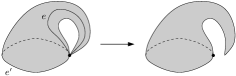
  (a) Pushing away from the boundary vertex

  

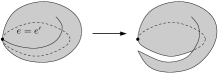
  (b) Pushing away from the boundary edge

  Figure 14. Pushing the interior of a cone away from its boundary

• If edges $e^{\prime}$ and $e$ are identified, then the edge on the boundary of the cone is identified with the “radius” edge leading to the apex of the cone, as illustrated in Figure 14(b). Once again we make the disc embedded, this time by pushing the interior of the disc away from the boundary edge, as illustrated.

In either case we obtain an embedded disc bounded by the edge $e^{\prime}$, which contradicts the first result above. ∎

References

- [1] M. V. Andreeva, I. A. Dynnikov, and K. Polthier, A mathematical webservice for recognizing the unknot, Mathematical Software: Proceedings of the First International Congress of Mathematical Software, World Scientific, 2002, pp. 201–207.
- [2] Benjamin A. Burton, Face pairing graphs and 3-manifold enumeration, J. Knot Theory Ramifications 13 (2004), no. 8, 1057–1101.
- [3] by same author, Introducing Regina, the 3-manifold topology software, Experiment. Math. 13 (2004), no. 3, 267–272.
- [4] by same author, Quadrilateral-octagon coordinates for almost normal surfaces, Experiment. Math. 19 (2010), no. 3, 285–315.
- [5] by same author, Computational topology with Regina: Algorithms, heuristics and implementations, Geometry and Topology Down Under (Craig D. Hodgson, William H. Jaco, Martin G. Scharlemann, and Stephan Tillmann, eds.), Contemporary Mathematics, no. 597, Amer. Math. Soc., Providence, RI, 2013.
- [6] Benjamin A. Burton, Ryan Budney, William Pettersson, et al., Regina: Software for 3-manifold topology and normal surface theory, http://regina.sourceforge.net/, 1999–2013.
- [7] Benjamin A. Burton, Alexander Coward, and Stephan Tillmann, Computing closed essential surfaces in knot complements, SCG ’13: Proceedings of the 29th Annual Symposium on Computational Geometry, ACM, 2013, pp. 405–414.
- [8] Benjamin A. Burton and Melih Ozlen, A fast branching algorithm for unknot recognition with experimental polynomial-time behaviour, Preprint, arXiv:1211.1079, November 2012.
- [9] Benjamin A. Burton, J. Hyam Rubinstein, and Stephan Tillmann, The Weber-Seifert dodecahedral space is non-Haken, Trans. Amer. Math. Soc. 364 (2012), no. 2, 911–932.
- [10] Bruce Randall Donald and David Renpan Chang, On the complexity of computing the homology type of a triangulation, 32nd Annual Symposium on Foundations of Computer Science (San Juan, PR, 1991), IEEE Comput. Soc. Press, Los Alamitos, CA, 1991, pp. 650–661.
- [11] Jean-Guillaume Dumas, Frank Heckenbach, David Saunders, and Volkmar Welker, Computing simplicial homology based on efficient Smith normal form algorithms, Algebra, Geometry, and Software Systems, Springer, Berlin, 2003, pp. 177–206.
- [12] Jim Fowler, Finding 0-efficient triangulations of 3-manifolds, Senior honors thesis, Harvard University, 2003.
- [13] Wolfgang Haken, Theorie der Normalflächen, Acta Math. 105 (1961), 245–375.
- [14] by same author, Über das Homöomorphieproblem der 3-Mannigfaltigkeiten. I, Math. Z. 80 (1962), 89–120.
- [15] William Jaco, The homeomorphism problem: Classification of 3-manifolds, Lecture notes, Available from http://www.math.okstate.edu/~jaco/pekinglectures.htm, 2005.
- [16] William Jaco and J. Hyam Rubinstein, 0-efficient triangulations of 3-manifolds, J. Differential Geom. 65 (2003), no. 1, 61–168.
- [17] William Jaco and Eric Sedgwick, Decision problems in the space of Dehn fillings, Topology 42 (2003), no. 4, 845–906.
- [18] William Jaco and Jeffrey L. Tollefson, Algorithms for the complete decomposition of a closed -manifold, Illinois J. Math. 39 (1995), no. 3, 358–406.
- [19] Tao Li, An algorithm to determine the Heegaard genus of a 3-manifold, Geom. Topol. 15 (2011), no. 2, 1029–1106.
- [20] Bruno Martelli and Carlo Petronio, Three-manifolds having complexity at most 9, Experiment. Math. 10 (2001), no. 2, 207–236.
- [21] by same author, A new decomposition theorem for 3-manifolds, Illinois J. Math. 46 (2002), 755–780.
- [22] Sergei Matveev, Algorithmic topology and classification of 3-manifolds, Algorithms and Computation in Mathematics, no. 9, Springer, Berlin, 2003.
- [23] Sergei V. Matveev, Complexity theory of three-dimensional manifolds, Acta Appl. Math. 19 (1990), no. 2, 101–130.
- [24] by same author, Tables of 3-manifolds up to complexity 6, Max-Planck-Institut für Mathematik Preprint Series (1998), no. 67, available from http://www.mpim-bonn.mpg.de/html/preprints/preprints.html.
- [25] J. Hyam Rubinstein, An algorithm to recognize the -sphere, Proceedings of the International Congress of Mathematicians (Zürich, 1994), vol. 1, Birkhäuser, 1995, pp. 601–611.
- [26] by same author, An algorithm to recognise small Seifert fiber spaces, Turkish J. Math. 28 (2004), no. 1, 75–87.
- [27] William P. Thurston, The geometry and topology of 3-manifolds, Lecture notes, Princeton University, 1978.