New limits on neutrino magnetic moment through non-vanishing 13-mixing

Abstract

The relatively large value of neutrino mixing angle $\theta_{13}$ set by recent measurements allows us to use solar neutrinos to set a limit on neutrino magnetic moment involving second and third families, $\mu_{\mu\tau}$. The existence of a random magnetic field in solar convective zone can produce a significant anti-neutrino flux when a non-vanishing neutrino magnetic moment is assumed. Even if we consider a vanishing neutrino magnetic moment involving the first family, electron anti-neutrinos are indirectly produced through the mixing between first and third families and $\mu_{\mu\tau}\neq 0$. Using KamLAND limits on the solar flux of electron anti-neutrino, we set the limit $\mu_{\mu\tau}<0.5\times 10^{-11}\mu_{B}$ for a reasonable assumption on the behavior of solar magnetic fields. This is the first time a limit on $\mu_{\mu\tau}$ is established in the literature directly from neutrino interaction with magnetic fields, and, interestingly enough, is comparable with the limits on neutrino magnetic moment involving the first family and with the ones coming from modifications on electroweak cross section.

I Introduction

In a recent paper Guzzo:2005rr we performed an analysis of how a non-vanishing neutrino transition magnetic moment involving second and third families, $\mu_{\mu\tau}$, could affect the flavour conversion of solar neutrinos. At that time we assumed a vanishing $\theta_{13}$, which allowed to produce a large flux of non-electronic anti-neutrinos, and our model was not limited by the absence of electron anti-neutrinos $\bar{\nu}_{e}$ in solar neutrino flux, as required by Kamland Eguchi:2003gg .

However, in that paper it was argued that a non-vanishing $\theta_{13}$ would open a channel for the production of electron anti-neutrinos, and then a limit on $\mu_{\mu\tau}$ could be established from the absence of a signal of $\bar{\nu}_{e}$ in solar neutrino flux. Since recent data indicates a relatively large value for this angle, we examine such limits in light of this new measurements.

II Conversion Probabilities

To calculate the probability that a electron neutrino produced at the sun evolves into an electron anti-neutrino in the presence of transition magnetic moments, in principle we would have to work using a 6$\times$6 evolution matrix formalism, involving $\nu_{a}=(\nu_{e},\nu_{\mu},\nu_{\tau},\bar{\nu}_{e},\bar{\nu}_{\mu},\bar{\nu}_{\tau})^{T}$. But the system can be simplified in specific cases. For instance, in Guzzo:2005rr we assumed a vanishing value for $\theta_{13}$, and rotating out the $23$-mixing with the definition $\nu^{\prime}=U_{23}^{-1}\nu$, the system was decoupled into two 3$\times$3 systems, which can be presented with a convenient reordering of eigenstates as:

$$i{\frac{\displaystyle{\ d}}{\displaystyle{\ dt}}}\left(\begin{array}[]{c}\nu_{e}\\ \nu_{\mu}^{\prime}\\ \bar{\nu}^{\prime}_{\tau}\\ \bar{\nu}_{e}\\ \bar{\nu}^{\prime}_{\mu}\\ \nu_{\tau}^{\prime}\end{array}\right)= \left(\begin{array}[]{cc}\left[\begin{array}[]{ccc}&&\\ &A&\\ &&\end{array}\right]&\begin{array}[]{ccc}&&\\ &0&\\ &&\end{array}\\ \begin{array}[]{ccc}&&\\ &0&\\ &&\end{array}&\left[\begin{array}[]{ccc}&&\\ &\tilde{A}&\\ &&\end{array}\right]\end{array}\right)\left(\begin{array}[]{c}\nu_{e}\\ \nu_{\mu}^{\prime}\\ \bar{\nu}^{\prime}_{\tau}\\ \bar{\nu}_{e}\\ \bar{\nu}^{\prime}_{\mu}\\ \nu_{\tau}^{\prime}\end{array}\right)$$ (27)

where

$$A=\left(\begin{array}[]{ccc}-\delta\cos 2\theta_{12}+V_{CC}+V_{NC}&\delta\sin 2\theta_{12}&0\\ \delta\sin 2\theta_{12}&\delta\cos 2\theta_{12}+V_{NC}&\mu_{\mu\tau}B\\ 0&\mu_{\mu\tau}B&-\Delta-V_{NC}\end{array}\right)$$ (28)

and $\tilde{A}$ is the same as $A$ with a change of sign on matter potentials. $\nu_{\mu}^{\prime}$ and $\nu_{\tau}^{\prime}$ are linear combinations of weak states as $\nu_{\mu}^{\prime}=cos\,\theta_{23}\,\nu_{\mu}-sin\,\theta_{23}\,\nu_{\tau}$, $\nu_{\tau}^{\prime}=sin\,\theta_{23}\,\nu_{\mu}+cos\,\theta_{23}\,\nu_{\tau}$, and with similar definitions to anti-neutrinos $\bar{\nu}$. Also, $\delta=\Delta m^{2}_{21}/4E$, $\Delta=\Delta m^{2}_{32}/4E$, and $V_{CC}$ and $V_{NC}$ are the charged current and neutral current interaction potentials with matter. Since all neutrinos in the sun are produced as electron neutrinos and the two systems are completely decoupled, no $\bar{\nu}_{e}$ was produced. For a regular magnetic field in the convective zone of the order of $100$ kG and for magnetic moments of the order of $10^{-11}$ $\mu_{B}$ we do not expect any transition to anti-neutrinos, since

$$\mu_{\mu\tau}B\sim 5.8\times 10^{-15}~{}{\rm eV}<<\Delta|_{E=10~{}{\rm MeV}}\sim 10^{-10}~{}{\rm eV}~{}.$$ (29)

However, random fluctuations of magnetic fields in convective zone are expected and promote the population of anti-neutrino states families Guzzo:2005rr . This is implemented through symmetric entries in Liouville equation, which induces decoherence, raising the $\nu\rightarrow\bar{\nu}$ conversion probability.

Nevertheless, when a non-vanishing value of $\theta_{13}$ is assumed, we can not decouple the system, and have to solve the full 6$\times$6 evolution equation. Rotating out both the mixing angles $\theta_{13}$ and $\theta_{23}$, we would have the following evolution matrix in the basis $\nu^{\prime}=U_{13}^{-1}U_{23}^{-1}\nu$ conveniently rearranged as in Eq. (27):

$$i{\frac{\displaystyle{\ d}}{\displaystyle{\ dt}}}\nu^{\prime}=\left(\begin{array}[]{cc}\left[A\right]&\left[\tilde{B}\right]\\ \left[B\right]&\left[\tilde{A}\right]\end{array}\right)\nu^{\prime}$$ (30)

with

$$A=\left(\begin{array}[]{ccc}-\delta\cos 2\theta_{12}+c_{13}^{2}V_{CC}+V_{NC}&\delta\sin 2\theta_{12}&0\\ \delta\sin 2\theta_{12}&+\delta\cos 2\theta_{12}+V_{NC}&\mu_{\mu\tau}Bc_{13}\\ 0&\mu_{\mu\tau}Bc_{13}&-\Delta-s^{2}_{13}V_{CC}-V_{NC}\\ \end{array}\right)$$ (31)

and

$$B=\left(\begin{array}[]{ccc}0&-\mu_{\mu\tau}Bs_{13}&-s_{13}c_{13}V_{CC}\\ -\mu_{\mu\tau}Bs_{13}&0&0\\ s_{13}c_{13}V_{CC}&0&0\end{array}\right)~{}.$$ (32)

where $s_{13}=\sin\theta_{13}$ and $c_{13}=\cos\theta_{13}$. $\tilde{A}$ ($\tilde{B}$) equals $A$ ($B$) by changing sign in matter potential terms. We will assume that the magnetic field is composed by a regular part and a random part. Again, for a regular magnetic field we do not expect significant production of anti-neutrinos. However, assuming a random component of the magnetic field, anti-neutrinos can be produced through different channels.

To include the random magnetic fields with the same procedure, we should use the density matrix formalism. From the $6\times 6$ Hamiltonian matrix, we get in the matrix density formalism a 35$\times$35 evolution system. Due to the complications of this procedure we will present later the full analysis of the system future , but we can get a good estimative assuming for now that the antineutrino production process will not be very different than in the scenario with vanishing $\theta_{13}$. Our procedure then would be to calculate the anti-neutrino production by the same assumption of last paper, a vanishing $\theta_{13}$, and then calculate the amount of $\bar{\nu}_{e}$ which is present in this anti-neutrino state in accordance with the measured value of $\theta_{13}$ An:2012eh ; Ahn:2012nd ; Abe:2011fz .

III Results

When we considered in Guzzo:2005rr that $\theta_{13}=0$, the $\bar{\nu}_{\tau}^{\prime}$ in Eq. (27) was identical to the mass eigenstate $\bar{\nu}_{3}$. As mentioned before, we will consider that the inclusion of a non-vanishing $\theta_{13}$ will not strongly change this production probability. However, the distribution of such anti-neutrino in the mass eigenstates is now:

$$\bar{\nu}_{\tau}^{\prime}=-(s_{13}c_{12})\nu_{1}-(s_{13}s_{12})\nu_{2}+(c_{13})\nu_{3}~{}.$$ (33)

Averaging out all terms involving oscillation between different mass scales when calculating the probabilities and assuming large values of the other mixing angles, we can write the electron anti-neutrino production as:

$$P(\nu_{e}\to\bar{\nu}_{e})\sim\sin^{2}\theta_{13}P(\nu_{e}\to\bar{\nu}_{\tau}^{\prime})|_{\theta_{13}=0}~{}.$$ (34)

KamLAND Eguchi:2003gg sets the strongest limit in the electronic anti-neutrino flux from the sun, given by $\phi(\bar{\nu}_{e})<3.7\times 10^{2}$ cm^-2s^-1. Writing in terms of a production probability and using solar model labeled GS98 in Serenelli:2011py where $\phi_{{}^{8}B}=5.6\times 10^{6}$ cm^-2s^-1, we obtain an upper limit of the electronic anti-neutrino production of $P<6.6\times 10^{-5}$. Considering all recent measurements of $\sin^{2}\theta_{13}$ An:2012eh ; Ahn:2012nd ; Abe:2011fz , we will use the value of best fit point GonzalezGarcia:2012sz $\sin^{2}\theta_{13}=2.5\times 10^{-2}$ in our analysis. This translates into a limit on anti-neutrino production of:

$$P(\nu_{e}\to\bar{\nu}^{\prime}_{\tau})|_{\theta_{13}=0}<2.7\times 10^{-3}~{}.$$ (35)

To calculate the anti-neutrino production probability we follow the procedure presented at Guzzo:2005rr . The probability is a function of the parameter

$$k=<(\mu B_{\perp})^{2}>L_{0}$$ (36)

where $L_{0}$ is a length scale related to the spatial coherence of the magnetic fluctuations. Rewriting $k$ in convenient units, we have:

$$k=3.4\times 10^{-17}\left[\frac{\mu}{10^{-11}\mu_{B}}\right]^{2}\left[\frac{B}{100\,{\rm kG}}\right]\left[\frac{L_{0}}{200\,{\rm km}}\right]\,{\rm eV}~{}.$$ (37)

We solved the evolution equation numerically assuming a vanishing $\theta_{13}$, as in Guzzo:2005rr . In Fig. 1 we present the conversion probability of anti-neutrinos if we assume a vanishing $\theta_{13}$, together with the limits on this probability that can be inferred from KamLAND data and the measured values of $\theta_{13}$, as presented in Eq. (35). The parameter region where the anti-neutrino production probability is larger than the KamLAND limit is excluded.

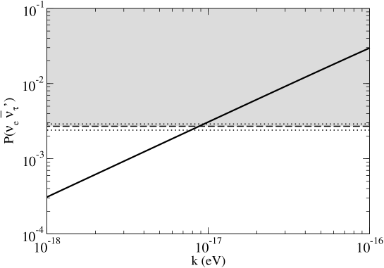
Figure 1: We present here the comparison between KamLAND limits on anti-neutrino production with the predictions of such production in our model. The solid line corresponds to the anti-neutrino production probability in the Sun, in the assumption of a vanishing $\theta_{13}$. The dashed line corresponds to the limits set by KamLAND on solar electronic anti-neutrino flux, converted to a limit on non-electronic anti-neutrino probability conversion, using $\sin^{2}\theta_{13}=0.025\pm 0.0023$ (1$\sigma$) GonzalezGarcia:2012sz . The dotted lines are obtained with the 1$\sigma$ limits for this angle.

From Fig. 1 we can extract a limit on $k$:

$$k<8\times 10^{-18}\,{\rm eV}~{},$$ (38)

which leads, from Eq. 37 to the following limit on magnetic field parameters:

$$\left[\frac{\mu}{10^{-11}\mu_{B}}\right]^{2}\left[\frac{B}{100\,{\rm kG}}\right]\left[\frac{L_{0}}{200\,{\rm km}}\right]\,{\rm eV}<0.24$$ (39)

For a reasonable assumption on magnetic field profile, i.e. a $100$ kG regular magnetic field with random fluctuations proportional to the regular one, and a $200$ km coherent length scale for such fluctuations, we translate this limit to:

$$\mu_{\mu\tau}<0.5\times 10^{-11}\mu_{B}~{}.$$ (40)

Such a limit can be compared with the ones coming from modifications on neutrino electroweak cross section Grimus:2002vb ; Liu:2004ny ; Montanino:2008hu ; Arpesella:2008mt , which applies for a combination on all neutrino magnetic moment elements. Although our limit is more stringent then the one reported for instance in Arpesella:2008mt , it depends on both the solar magnetic field profile and the characteristics of its random fluctuations.

IV Conclusions

In this work we set a limit on the neutrino transition magnetic moment involving the second and third families using solar neutrino data and assuming a specific profile for the solar magnetic field. For a vanishing mixing angle $\theta_{13}$ we could only set loose bounds on such magnetic moment due to the electron anti-neutrino flavour decoupling on neutrino evolution equation. Now with a reasonable high measured value for such angle, a stringent limit was established, for the first time from the direct interaction of neutrinos with magnetic fields, at the same order of magnitude of the limits involving the first neutrino family and the limits coming from modifications on electroweak cross section.

Some approximations were made in the calculations that allowed us to use a previous study to calculate the anti-neutrino appearance probability. We plan to critically evaluate such approximations in a future work, but we expect that the limits established here are conservative, and a more detailed analysis could open other channels of anti-neutrino production, improving the limit presented here.

References

- (1) M. M. Guzzo, P. C. de Holanda and O. L. G. Peres, Phys. Rev. D 72, 073004 (2005) [hep-ph/0504185].
- (2) K. Eguchi et al. [KamLAND Collaboration], Phys. Rev. Lett. 92, 071301 (2004) [hep-ex/0310047].
- (3) A. M. Serenelli, W. C. Haxton, C. Peña-Garay, Astrophys.J. 743 (2011) 24.
- (4) M. M Guzzo, P. C. de Holanda,O. L. G. Peres and R. Picoreti, work in preparation.
- (5) M. C. Gonzalez-Garcia, M. Maltoni, J. Salvado and T. Schwetz, arXiv:1209.3023 [hep-ph].
- (6) F. P. An et al. [DAYA-BAY Collaboration], Phys. Rev. Lett. 108, 171803 (2012) [arXiv:1203.1669 [hep-ex]].
- (7) J. K. Ahn et al. [RENO Collaboration], Phys. Rev. Lett. 108, 191802 (2012) q [arXiv:1204.0626 [hep-ex]].
- (8) Y. Abe et al. [DOUBLE-CHOOZ Collaboration], Phys. Rev. Lett. 108, 131801 (2012) [arXiv:1112.6353 [hep-ex]].
- (9) W. Grimus, M. Maltoni, T. Schwetz, M. A. Tortola and J. W. F. Valle, Nucl. Phys. B 648, 376 (2003) [hep-ph/0208132].
- (10) D. W. Liu et al. [Super-Kamiokande Collaboration], Phys. Rev. Lett. 93, 021802 (2004) [hep-ex/0402015].
- (11) D. Montanino, M. Picariello and J. Pulido, Phys. Rev. D 77, 093011 (2008) [arXiv:0801.2643 [hep-ph]].
- (12) C. Arpesella et al. [Borexino Collaboration], Phys. Rev. Lett. 101, 091302 (2008) [arXiv:0805.3843 [astro-ph]].