Solution to the Sigma-Problem of Pulsar Wind Nebulae.

Abstract

We present first results of three dimensional relativistic magnetohydrodynamical simulations of Pulsar Wind Nebulae. They show that the kink instability and magnetic dissipation inside these nebulae may be the key processes allowing to reconcile their observations with the theory of pulsar winds. In particular, the size of the termination shock, obtained in the simulations, agrees very well with the observations even for Poynting-dominated pulsar winds. Due to magnetic dissipation the total pressure in the simulated nebulae is particle-dominated and more or less uniform. While in the main body of the simulated nebulae the magnetic field becomes rather randomized, close to the termination shock, it is dominated by the regular toroidal field freshly-injected by the pulsar wind. This field is responsible for driving polar outflows and may explain the high polarization observed in pulsar wind nebulae.

1 Introduction

It is now well established that Pulsar Wind Nebulae (PWN) are powered by relativistic winds from neutron stars, formed during violent deaths of massive normal stars. Theory of such winds, based on the physical processes in the magnetospheres of neutron stars, predicts that they are strongly Poynting-dominated at their base (see Arons, 2012, and references therein).

However, simple one-dimensional models of PWN fit the observations only if pulsar winds are particle-dominated. Quantitatively this conflict is best described using the wind magnetization parameter $\sigma$ defined as the ratio of the wind Poynting flux to its kinetic energy flux. Theoretical models of pulsar magnetospheres and wind predict $\sigma\gg 1$, whereas the 1D models of PWN suggest $\sigma\sim 10^{-3}$ (Rees & Gunn, 1974; Kennel & Coroniti, 1984; Emmering & Chevalier, 1987; Begelman & Li, 1992). A slightly higher magnetization, $\sigma\sim 10^{-2}$, was later suggested by axisymmetric numerical simulations (Komissarov & Lyubarsky, 2003, 2004; Del Zanna et al., 2004; Bogovalov et al., 2005).

Several possible explanations of this $\sigma$-problem have been put forward over the years. The simplest one is that the electromagnetic energy of the pulsar wind is converted into kinetic energy of the wind on its way from the pulsar to the wind termination shock, where freshly supplied plasma is injected into the PWN. Although claims have been made that ideal MHD acceleration mechanisms can provide the required energy conversion (e.g. Vlahakis, 2004), it has now become clear that this is not the case (e.g. Komissarov et al., 2009; Lyubarsky, 2009, 2010).

The acceleration can be facilitated via non-ideal processes, involving magnetic dissipation, in pulsar winds (Coroniti, 1990). For the wind of the Crab pulsar, the dissipation length scale still significantly exceeds the radius of the wind termination shock (Lyubarsky & Kirk, 2001), unless the pulsar produces much more plasma compared to the predictions of the current models of pair-production in pulsar magnetospheres (see Arons, 2012, and references therein). Alternatively, the energy associated with the alternating component of magnetic field of the striped wind can be rapidly dissipated at the termination shock itself (Lyubarsky, 2003; Sironi & Spitkovsky, 2011). Although the striped-wind model allows conversion of a large fraction of the total Poynting flux into the internal energy of PWN plasma, much more is needed to approach the target value of $\sigma\sim 10^{-3}\div 10^{-2}$. Indeed, the dissipation is confined to the striped zone of the wind and only the alternating component of magnetic field dissipates. Closer to the poles, the magnetization of pulsar wind plasma remains very high even after it crosses the termination shock and, as a result, the overall magnetization of plasma injected into the nebula is much higher than that of the Kennel-Coroniti model, unless the striped zone spreads over almost the entire wind, implying that the pulsar is an almost orthogonal rotator (Coroniti, 1990; Komissarov, 2012).

In contrast to these ideas, Begelman (1998) argued that the 1D models of PWN could be highly unrealistic and their predictions not trustworthy. He has shown that the plasma configuration assumed in these models is unstable to the magnetic kink instability and speculated that the disrupted configuration may be less demanding on the magnetization of pulsar winds. Indeed, one would expect the magnetic pressure due to randomized magnetic field to dominate the mean Maxwell stress tensor, and the adiabatic compression to have the same effect on the magnetic pressure as on the thermodynamic pressure of relativistic gas. Under such conditions, the global dynamics of PWN produced by high-$\sigma$ winds may not be that much different from those of PWN produced by particle-dominated winds. These expectations have received strong support from the recent numerical studies (Mizuno et al., 2011) of magnetic kink-instability of the cylindrical magnetostatic configuration, which was used in Begelman & Li (1992) to model PWN. These simulations have shown a relaxation towards quasi-uniform total pressure distribution inside the computational domain on the dynamical time-scale. Mizuno et al. (2011) also reported a significant magnetic dissipation.

The most important factor missing in the simulations by Mizuno et al. (2011) is the continuous injection of magnetic flux and energy in PWN by their pulsar winds. As a result, there is no termination shock whose size is an important parameter used to test theories of PWN against the observational data. The observed strong polarization of PWN is suggestive of significant regular magnetic field in the form of concentric loops in their central regions, which could have been supplied by the pulsar wind relatively recently. The polar jets, most prominent in the Crab and Vela nebulae are best explained by the action of magnetic hoop stress of such fields (Lyubarsky, 2002; Komissarov & Lyubarsky, 2003; Del Zanna et al., 2004; Bogovalov et al., 2005). Thus, the next logical step is to carry out 3D numerical simulations of PWN proper, similar in their setup to the previous axisymmetric simulations. We are currently conducting such studies and here report its first most interesting results.

2 Simulation setup

Initially, the computational domain is split in two zones separated by a spherical boundary of radius $r_{i}=10^{18}$cm. The outer zone is filled with radially-expanding cold supernova ejecta. The solution in this zone has Hubble’s velocity profile

$$v=v_{\rm{i}}\left(\frac{r}{r_{\rm{i}}}\right)$$ (1)

and constant density $\rho_{\rm{e}}$. The values of parameters $\rho_{\rm{e}}$ and $v_{\rm{i}}$ are determined using the observed expansion rate of the Crab nebula and typical parameters of type-II supernovae. The inner zone is initially filled with unshocked pulsar wind. In our model of the wind, we assume that the alternating component of magnetic field in its striped zone has completely dissipated along the way from the pulsar to the PWN. Although this may not be the case and most of the dissipation occurs instead at the termination shock, dynamically this makes no difference (Lyubarsky, 2003). The total energy flux density of the wind follows that of the monopole model (Michel, 1973)

$$f_{\rm tot}(r,\theta)\propto\left(\frac{1}{r^{2}}\right)\left(\sin^{2}\theta+b\right)\,.$$ (2)

The parameter $b=0.03$ is added for numerical reasons. This energy is divided into magnetic, $f_{\rm m}$, and kinetic, $f_{\rm k}$, terms

$$f_{\rm m}(r,\theta)=\sigma(\theta)\frac{f_{\rm tot}(\theta,r)}{1+\sigma(\theta)},\quad f_{\rm k}(r,\theta)=\frac{f_{\rm tot}(r,\theta)}{1+\sigma(\theta)}\,,$$ (3)

where $\sigma(\theta)$ is the latitude dependent wind magnetization.

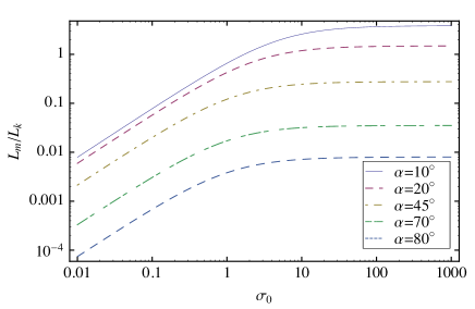
Figure 1: Electromagnetic luminosity over kinetic luminosity injected into the PWN against value before reconnection $\sigma_{0}$ for various angles of obliqueness $\alpha$. If the obliqueness is larger than $\sim 45^{\circ}$, the luminosity fraction saturates at approximately this value. This is why our dynamical simulations can also provide reasonable models for highly magnetized cases with $\sigma_{0}>10^{3}$.

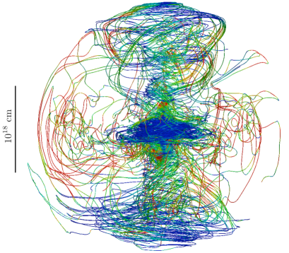
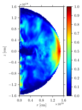
Figure 2: Left panel: 3D rendering of the magnetic field structure in the model with $\sigma_{0}=3$ at $t\simeq 70\rm~{}years$ after the start of the simulation. Magnetic field lines are integrated from sample points starting at $r=3\times 10^{17}\rm cm$. Colors indicate the dominating field component, blue for toroidal and red for poloidal. Right panel: Azimuthally averaged $\bar{\alpha}\equiv\langle B_{p}^{2}/B^{2}\rangle_{\phi}$ for the same model.

For simplicity, we assume that before dissipation of magnetic stripes the wind magnetization saturates at

$$\tilde{\sigma}_{0}(\theta)=\left\{\begin{array}[]{ll}\left(\theta/\theta_{\rm 0}\right)^{2}\ \sigma_{0};&\theta\leq\theta_{\rm 0}\\ \sigma_{0};&\theta>\theta_{\rm 0}\end{array}\right.$$ (6)

where the additional (small) parameter $\theta_{0}=10^{\circ}$ was introduced to ensure that the Poynting flux vanishes on the axis for an axisymmetric model. Dissipation of magnetic stripes changes the magnetization of the striped wind zone so that

$$\sigma(\theta)=\frac{\tilde{\sigma}_{0}(\theta)\chi_{\alpha}(\theta)}{1+\tilde{\sigma}_{0}(\theta)(1-\chi_{\alpha}(\theta))}\,,$$ (7)

where

$$\chi_{\alpha}(\theta)=\left\{\begin{array}[]{ll}(2\phi_{\alpha}(\theta)/\pi-1)^{2},&\pi/2-\alpha<\theta<\pi/2+\alpha\\ 1,&\mbox{otherwise}\end{array}\right.,$$ (8)

with $\phi_{\alpha}(\theta)\equiv\arccos(-\cot(\theta)\cot(\alpha))$. Here, $\alpha$ signifies the magnetic inclination angle of the pulsar which determines the size of the striped wind zone (Komissarov, 2012). Figure 1 shows the ratio of the wind total electromagnetic luminosity to its total kinetic luminosity, obtained via integration of the fluxes given by Eqs. 3, as a function of $\sigma_{0}$ for different values of the magnetic inclination angle. In this letter we present simulations with $\sigma_{0}=0.01,1,3$ and $\alpha=45^{o}$. As one can see in Fig. 1, for $\sigma_{0}=3$ the luminosity ratio is already very close to the asymptotic value in the limit $\sigma_{0}\to\infty$, which is determined by the extent of the striped wind zone for all except very small values of $\alpha$. This is why we expect our models with $\sigma_{0}=3$ not to be very different from those with much higher $\sigma_{0}$, which can be found in real pulsar winds.

The wind’s magnetic field is purely azimuthal and changes direction at the equatorial plane. Its strength, as measured in the pulsar frame, is found via

$$B_{\phi}(r,\theta)=\pm\sqrt{4\pi f_{\rm m}(r,\theta)/v}\,,$$ (9)

where $v$ is the radial wind velocity. For simplicity, we adopt the same value of the wind Lorentz factor, $\Gamma=10$, for all its streamlines. Hence the numerical wind density follows as

$$\rho(r,\theta)=f_{\rm k}(r,\theta)/(\Gamma^{2}c^{2}v).$$ (10)

When the simulations begin, the discontinuity at $r_{\rm{i}}$ between these two initial zones splits and the termination shock first rapidly moves inside towards the wind origin, reflecting the artificial nature of our initial configuration. Soon after, it re-bounces and begins to expand at a much slower rate, gradually approaching its asymptotic self-similar position (Rees & Gunn, 1974). For an unmagnetized wind, $\sigma_{0}=0$, its equatorial radius at this stage evolves as

$$r_{0}\simeq\sqrt{2}r_{\rm n}\left(\frac{v_{\rm n}}{c}\right)^{1/2}\left(1-\left(1+\frac{v_{\rm{n}}t}{r_{\rm{i}}}\right)^{-2}\right)^{-1/2}\,,$$ (11)

where $v_{\rm{n}}$ is the expansion rate of the PWN, and $t$ is the time since the start of the simulations. One can see that the time-scale of transition to the self-similar expansion is $\sim r_{\rm{i}}/v_{\rm{i}}$, which is $\simeq 210~{}$yr for the parameters of our simulations. We do not yet fully reach the self-similar phase in 3D simulations and hence use this solution as a reference.

The simulations are performed with MPI-AMRVAC (Keppens et al., 2012), solving the set of special relativistic magneto-hydrodynamic conservation laws in cartesian geometry. We employ a cubic domain with edge length of $2\times 10^{19}\rm cm$, large enough to contain today’s Crab nebula. Outflow boundary conditions allow plasma to leave the simulation box. The adaptive mesh refinement starts at a base level of $64^{3}$ cells and is used to resolve the expanding nebula bubble with a cell-size of $\Delta x=1.95\times 10^{16}\rm cm$ (on the fifth level). Special action is taken to properly resolve the termination shock and the flow near the origin. To this end, additional grid levels centered on the termination shock are automatically activated, depending on the shock size. For the simulations shown here, the shock is thus resolved by $3-4$ extra grid-levels (resulting in $8-9$ levels in total) on which we employ a more robust minmod reconstruction in combination with Lax-Friedrich flux splitting. 2D comparison simulations are performed with equivalent numerical setup and differ only in the use of cylindrical coordinates in the $r,z$-plane.

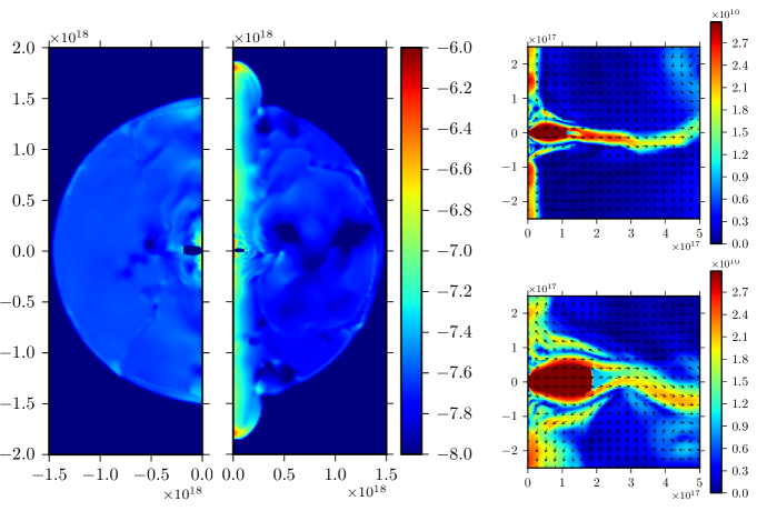
Figure 3: Left panel: The total pressure distribution in the 3D (left hemisphere) and the corresponding 2D (right hemisphere) solutions for the same model with $\sigma_{0}=3$ at $t\simeq 70\rm~{}years$. Right panels: Velocity magnitude and direction for the same solutions, with the 2D one at the top and 3D one at the bottom. Note the scale difference between left/right panels.

3 Results

In basic agreement with the simulations by Mizuno et al. (2011), the highly organized coaxial configuration of magnetic field, characteristic of previous 2D simulations of PWN, is largely destroyed in our 3D models. However, the azimuthal component is still dominant in the vicinity of the termination shock, in the region roughly corresponding to Crab’s torus (see Figure 2), which is filled mainly with “fresh” plasma which is just on its way from the termination shock to the main body of the nebula. As we have pointed out in the introduction, the emission of this plasma could be behind the strong polarization observed in the central region of the Crab nebula. This figure also shows predominantly poloidal magnetic field in the outskirts of PWN, close to the equator. However, the magnetic field is rather weak in this region.

Also in agreement with Mizuno et al. (2011), the total pressure distribution of our 3D solutions is much more uniform compared to 2D solutions of the same problem. As a result, the expansion of PWN in 3D is more or less isotropic, whereas in 2D the artificially enhanced axial compression due to the magnetic hoop stress promotes noticeably faster expansion in the polar direction. As one can see in Figure 3, by the end of the simulations, the 2D solution with $\sigma_{0}=3$ begins to exhibit a jet breakout, similar to those observed in the earlier 2D simulations of highly-magnetized young PWN of magnetars (Bucciantini et al., 2007, 2008), with application to Gamma Ray Bursts.

Figure 4 shows the evolution of the equatorial radius of the termination shock with time in all our simulations together with the analytical prediction from Eq. 11. We anticipated that in 3D the shock radius turns out similar to that given by the analytical model for unmagnetized wind, as this was suggested in Begelman (1998). This is indeed the case, but Figure 4 also shows that the size of the termination shock exhibits only a weak dependence on the initial magnetization $\sigma_{0}$, once $\sigma_{0}\geq 1$. However, we also expected to find a much smaller shock radius in 2D simulations, as their symmetry prevents the development of the key process in the Begelman’s theory, the kink instability. What we have actually found is that, although in our 2D simulations the shock radius is indeed smaller, the difference is not dramatic.

An explanation for this result is suggested by Figure 5, which shows the ratio of magnetic to thermal energy of simulated PWN in our numerical models. One can see that, not only do our 3D solutions exhibit significant magnetic dissipation, which agrees with Mizuno et al. (2011), but the 2D solutions do as well. Indeed, for 2D models with $\sigma_{0}=1,3$ this parameter decreases from $\sim 0.3$, which is close to the mean value of freshly-injected plasma (Komissarov, 2012), to $\sim 0.03$. Such a low value means that the total pressure in the nebula is dominated by the gas pressure, just like in models with particle-dominated winds, and this is why the shock radius is close to that of the unmagnetized model. The property of our 2D models which makes magnetic dissipation possible is the opposite orientation of magnetic loops in the northern and southern hemispheres, in contrast with most previous 2D simulations which were limited to only one hemisphere. Strong mixing between the two hemispheres, discovered already in Camus et al. (2009), reduces the characteristic length scale of magnetic inhomogeneities and speeds up the magnetic dissipation. The displacement of magnetic loops near the polar axis via the kink instability is an additional way of facilitating magnetic dissipation in 3D models. This agrees with the observed lower level of magnetic energy inside PWN in these models (see Figure 5).

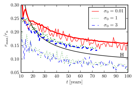
Figure 4: Shock size in the equatorial plane for the two- (thin lines) and three-dimensional case (thick lines). The solid black curve labeled “H” follows the hydrodynamic prediction according to Eq. 11.

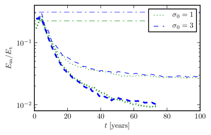
Figure 5: Ratio of the total magnetic energy to the total thermal energy of PWN as a function of time for 2D (thin lines) and 3D (thick lines) models. Horizontal dash-dotted lines indicate the expected ratios at the self-similar phase in the absence of magnetic dissipation (Komissarov, 2012).

The data presented in Figure 3 show that the axial compression remains a feature of our 3D-solution near the termination shock and that the “tooth-paste” effect of hoop-stress due to freshly-injected azimuthal magnetic field of the pulsar wind is still capable of driving polar jets. But compared to the 2D models, the region of operation of this jet-production mechanism is much more compact.

4 Discussion

The results of our simulations provide strong support to Begelman’s hypothesis that the essence of the sigma-problem of PWN relies in the inadequacy of using over-simplified models. He argued that these models were unstable to kink modes and that randomization of magnetic field, resulting from this instability, would lead to a termination shock of size similar to that of weakly-magnetized models, even if the actual magnetization was still very high. Our results confirm, and augment this by showing that the magnetization may actually be significantly reduced via onset of magnetic dissipation accompanying randomization of magnetic field. The observed properties of PWN may mimic those of models with weakly magnetized winds not because magnetic stress of randomized magnetic field effectively reduces to pressure but because the magnetic dissipation renders the PWN gas-pressure-dominated (high-$\beta$ plasma). In fact, high-magnetization of PWN plasma seems to be ruled out by the observations of synchrotron and inverse-Compton emission of the Crab nebula, which show that the magnetic field is energetically sub-dominant to the population of relativistic electrons by a factor of $\sim 30$ (Hillas, 1998).

Although the dissipation in the simulations ultimately is of numerical origin and occurs at the cell-size scale, the extreme resolution employed in a fully conservative, grid-adaptive computation can mimic processes creating such fine magnetic structures and hence the energy conversion has to be taken seriously. Moreover, the observed energy content of the Crab nebula does suggest efficient magnetic dissipation on a time scale which is significantly shorter than the age of the nebula but much longer compared to its Alfvén crossing time (Komissarov, 2012).

The dynamics of the inner region of our 3D numerical models is still strongly influenced by the regular magnetic field of freshly-injected plasma. The hoop stress of this field is still capable of producing noticeable axial compression close to the termination shock and driving polar outflows, required to explain the Crab jet, and jets of other PWN. However, these are much more moderate than in 2D models. It appears that the strong relativistic jets emerging in previous 2D simulations of magnetar bubbles, with application to Gamma Ray Bursts, may well be artifacts of the imposed axial symmetry.

5 Acknowledgments

SSK and OP are supported by STFC under the standard grant ST/I001816/1. SSK acknowledges support by the Russian Ministry of Education and Research under the state contract 14.B37.21.0915 for Federal Target-Oriented Program. RK acknowledges FWO-Vlaanderen, grant G.0238.12, and BOF F+ financing related to EC FP7/2007-2013 grant agreement SWIFF (no.263340).

References

- Arons (2012) Arons J., 2012, Sp.Sci.Rev., 33
- Begelman (1998) Begelman M. C., 1998, ApJ, 493, 291
- Begelman & Li (1992) Begelman M. C., Li Z.-Y., 1992, ApJ, 397, 187
- Bogovalov et al. (2005) Bogovalov S. V., Chechetkin V. M., Koldoba A. V., Ustyugova G. V., 2005, MNRAS, 358, 705
- Bucciantini et al. (2007) Bucciantini N., Quataert E., Arons J., Metzger B. D., Thompson T. A., 2007, MNRAS, 380, 1541
- Bucciantini et al. (2008) Bucciantini N., Quataert E., Arons J., Metzger B. D., Thompson T. A., 2008, MNRAS, 383, L25
- Camus et al. (2009) Camus N. F., Komissarov S. S., Bucciantini N., Hughes P. A., 2009, MNRAS, 400, 1241
- Coroniti (1990) Coroniti F. V., 1990, ApJ, 349, 538
- Del Zanna et al. (2004) Del Zanna L., Amato E., Bucciantini N., 2004, A&A, 421, 1063
- Emmering & Chevalier (1987) Emmering R. T., Chevalier R. A., 1987, ApJ, 321, 334
- Hillas (1998) Hillas A. M., 1998, ApJ, 503, 744
- Kennel & Coroniti (1984) Kennel C. F., Coroniti F. V., 1984, ApJ, 283, 694
- Keppens et al. (2012) Keppens R., Meliani Z., van Marle A., Delmont P., Vlasis A., van der Holst B., 2012, J.Comput.Phys., 231, 718
- Komissarov (2012) Komissarov S. S., 2012, ArXiv e-prints
- Komissarov & Lyubarsky (2003) Komissarov S. S., Lyubarsky Y. E., 2003, MNRAS, 344, L93
- Komissarov & Lyubarsky (2004) Komissarov S. S., Lyubarsky Y. E., 2004, MNRAS, 349, 779
- Komissarov et al. (2009) Komissarov S. S., Vlahakis N., Königl A., Barkov M. V., 2009, MNRAS, 394, 1182
- Lyubarsky (2009) Lyubarsky Y., 2009, ApJ, 698, 1570
- Lyubarsky & Kirk (2001) Lyubarsky Y., Kirk J. G., 2001, ApJ, 547, 437
- Lyubarsky (2002) Lyubarsky Y. E., 2002, MNRAS, 329, L34
- Lyubarsky (2003) Lyubarsky Y. E., 2003, MNRAS, 345, 153
- Lyubarsky (2010) Lyubarsky Y. E., 2010, MNRAS, 402, 353
- Michel (1973) Michel F. C., 1973, ApJ Lett., 180, L133
- Mizuno et al. (2011) Mizuno Y., Lyubarsky Y., Nishikawa K.-I., Hardee P. E., 2011, ApJ, 728, 90
- Rees & Gunn (1974) Rees M. J., Gunn J. E., 1974, MNRAS, 167, 1
- Sironi & Spitkovsky (2011) Sironi L., Spitkovsky A., 2011, ApJ, 741, 39
- Vlahakis (2004) Vlahakis N., 2004, ApJ, 600, 324