Adaptive tuning of Majorana fermions in a quantum dot chain.

Abstract

We suggest a way to overcome the obstacles that disorder and high density of states pose to the creation of unpaired Majorana fermions in one-dimensional systems. This is achieved by splitting the system into a chain of quantum dots, which are then tuned to the conditions under which the chain can be viewed as an effective Kitaev model, so that it is in a robust topological phase with well-localized Majorana states in the outermost dots. The tuning algorithm that we develop involves controlling the gate voltages and the superconducting phases. Resonant Andreev spectroscopy allows us to make the tuning adaptive, so that each pair of dots may be tuned independently of the other. The calculated quantized zero bias conductance serves then as a natural proof of the topological nature of the tuned phase.

I Introduction

Majorana fermions are the simplest quasiparticles predicted to have non-Abelian statistics.Ali12 ; Bee11 These topologically protected states can be realized in condensed matter systems, by making use of a combination of strong spin-orbit coupling, superconductivity, and broken time-reversal symmetry.Sau10 ; Ore10 ; Lut10 Recently, a series of experiments have reported the possible observation of Majorana fermions in semiconducting nanowires,Mou12 ; Den12 ; Das12 ; Rok12 attracting much attention in the condensed matter community.

Associating the observed experimental signatures exclusively with these non-Abelian quasiparticles, however, is not trivial. The most straightforward signature, the zero bias peak in Andreev conductanceBol07 ; Law09 is not unique to Majorana fermions, but can appear as a result of various physical mechanisms,Sas00 ; Pik12 ; Fle10 ; Kel12 ; Tew12 ; Pie12 ; Liu12 such as the Kondo effect or weak anti-localization. It has also been pointed out that disorder has a detrimental effect on the robustness of the topological phase, since in the absence of time-reversal symmetry it may close the induced superconducting gap.And59 This requires experiments performed with very clean systems. Additionally, the presence of multiple transmitting modes reduces the amount of control one has over such systems,Pot10 ; Sta11 ; Bro11 ; Rie12 and the contribution of extra modes to conductance hinders the observation of Majorana fermions.Wim11 Thus, nanowire experiments need setups in which only few modes contribute to conductance.

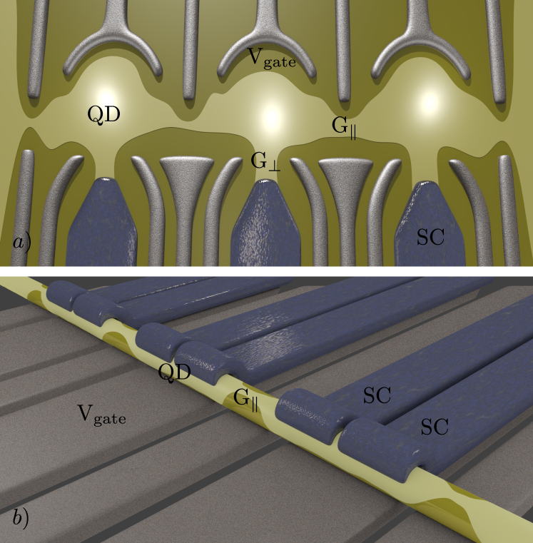
Figure 1: Examples of systems allowing implementation of a Kitaev chain. Panel (a): a chain of quantum dots in a 2DEG. The QDs are connected to each other, and to superconductors (labeled SC), by means of quantum point contacts. The first and the last dots are also coupled to external leads. The normal state conductance of quantum point contacts (QPCs) between adjacent dots or between the end dots and the leads is $G_{\parallel}$, and of the QPCs linking a dot to a superconductor is $G_{\perp}$. The confinement energy inside each QD can be controlled by varying the potential $V_{\rm gate}$. Panel (b): Realization of the same setup using a nanowire, with the difference that each dot is coupled to two superconductors in order to control the strength of the superconducting proximity effect without the use of QPCs.

In this work we approach the problem of realizing systems in a non-trivial topological phase from a different angle. We wish to emulate the Kitaev chain modelKit01 which is the simplest model exhibiting unpaired Majorana bound states. The proposed system consists of a chain of quantum dots (QDs) defined in a two-dimensional electron gas (2DEG) with spin orbit coupling, in proximity to superconductors and subjected to an external magnetic field. Our geometry enables us to control the parameters of the system to a great extent by varying gate potentials and superconducting phases. We will show how to fine tune the system to the so-called “sweet spot” in parameter space, where the Majorana fermions are well-localized at the ends of the system, making the topological phase maximally robust. A sketch of our proposed setup is presented in Fig. 1a).

The setup we propose and the tuning algorithm is not restricted solely to systems created in a two-dimensional electron gas. The essential components are the ability to form a chain of quantum dots and tune each dot separately. In semiconducting nanowires the dots can be formed from wire segments separated by gate-controlled tunnel barriers, and all the tuning can be done by gates, except for the coupling to a superconductor. This coupling, in turn, can be controlled by coupling two superconductors to each dot and applying a phase difference to these superconductors. The layout of a nanowire implementation of our proposal is shown in Fig. 1b).

This geometry has the advantage of eliminating many of the problems mentioned above. By using single level quantum dots, and also quantum point contacts (QPC) in the tunneling regime, we solve issues related to multiple transmitting modes. Additional problems, such as accidental closings of the induced superconducting gap due to disorder, are solved because our setup allows us to tune the system to a point where the topological phase is most robust, as we will show.

We present a step-by-step tuning procedure which follows the behavior of the system in parallel to that expected for the Kitaev chain. As feedback required to control every step we use the resonant Andreev conductance, which allows to track the evolution of the system’s energy levels. We expect that the step-by-step structure of the tuning algorithm should eliminate the large number of non-Majorana explanations of the zero bias peaks.

A related layout together with the idea of simulating a Kitaev chain was proposed recently by J. D. Sau and S. Das Sarma.Sau12 Although similar in nature, the geometry which we consider has several advantages. First of all, coupling the superconductors to the quantum dots in parallel, allows us to not rely on crossed Andreev reflection. More importantly, being able to control inter-dot coupling separately from all the other properties allows to address each dot or each segment of the chain electrically. This can be achieved by opening all the QPCs except for the ones that contact the desired dots.

This setup can also be extended to more complicated geometries which include T-junctions of such chains. Benefiting from the high tunability of the system and the localization of the Majorana fermions, it might then be possible to implement braidingAli11 ; Sau11 and demonstrate their non-Abelian nature.

The rest of this work is organized as follows. In section II we briefly review a generalized model of Kitaev chain, and identify the ”sweet spot” in parameter space in which the Majorana fermions are the most localized. The system of coupled quantum dots is described in section III. For the purpose of making apparent the resemblance of the system to the Kitaev chain, we present a simple model which treats each dot as having a single spinful level. We then come up with a detailed tuning procedure describing how one can control the parameters of the simple model, in order to bring it to the desired point in parameter space. In section IV our tuning prescription is applied to the suggested system of a chain of QDs defined in a 2DEG, and it is shown using numerical simulations that at the end of the process the system is indeed in a robust topological phase. We conclude in section V.

II Generalized Kitaev chain

In order to realize unpaired Majorana bound states, we start from the Kitaev chainKit01 generalized to the case where the on-site energies as well as the hopping terms are not uniform and can vary from site to site. The generalized Kitaev chain Hamiltonian is defined as

$$H_{\text{K}}=\sum_{n=1}^{L-1}\Big{[}\Big{(} t_{n}e^{i\theta_{n}}a^{\dagger}_{n+1}a_{n}+\Delta_{n}e^{i\phi_{n}}a^{\dagger}_{n+1}a^{\dagger}_{n}$$

$$+{h.c.}\Big{)}+\varepsilon_{n}a^{\dagger}_{n}a_{n}\Big{]},$$ (1)

where $a_{n}$ are fermion annihilation operators, $\varepsilon_{n}$ are the on-site energies of these fermions, $t_{n}\exp(i\theta_{n})$ are the hopping terms, and $\Delta_{n}\exp(i\phi_{n})$ are the p-wave pairing terms.

The chain supports two Majorana bound states localized entirely on the first and the last sites, when (i): $\varepsilon_{n}=0$, (ii): $\Delta_{n}=t_{n}$, and (iii) $\phi_{n+1}-\phi_{n}-\theta_{n+1}-\theta_{n}=0$. The larger values of $t_{n}$ lead to a larger excitation gap. The condition (iii) is equivalent, up to a gauge transformation, to the case where the hopping terms are all real, and the phases of the p-wave terms are uniform. The energy gap separating the Majorana modes from the first excited state then equals

$$E_{\text{gap}}=2\min\left\{t_{n}\right\}_{n}.$$ (2)

The above conditions (i)–(iii), constitute the “sweet spot” in parameter space to which we would like to tune our system. Since all of these conditions are local and only involve one or two sites, our tuning procedure includes isolating different parts of the system and monitoring their energy levels. For that future purpose we will use the expression for excitation energies of a chain of only two sites with $\varepsilon_{1}=\varepsilon_{2}=0$:

$$E_{12}=\pm(t_{1}\pm\Delta_{1}).$$ (3)

III System description and the tuning algorithm

The most straightforward way to emulate the Kitaev chain is to create an array of spinful quantum dots, and apply a sufficiently strong Zeeman field such that only one spin state stays close to the Fermi level. Then the operators of these spin states span the basis of the Hilbert space of the Kitaev chain. If we require normal hopping between the dots and do not utilize crossed Andreev reflection, then in order to have both $t_{n}$ and $\Delta_{n}$ nonzero we need to break the particle number conservation and spin conservation. The former is achieved by coupling each dot to a superconductor, the latter can be achieved by spatially varying Zeeman coupling,Cho11 ; Kja12 or more conventionally by using a material with a sufficiently strong spin-orbit coupling. Examples of implementation of such a chain of quantum dots in a two dimensional electron gas and in semiconducting nanowires are shown in Fig. 1.

We neglect all the levels in the dots except for the one closest to the Fermi level, which is justified if the level spacing in the dot is larger than all the other Hamiltonian terms. We neglect the Coulomb blockade, since we assume that the dot is strongly coupled to the superconducting lead. The general form of the BdG Hamiltonian describing such a chain of spinful single-level dots is then given by:

$$\begin{split}H_{\text{S}}&=\sum_{n,s,s^{\prime}}\left(\mu_{n}\sigma_{0}+V_{z}\sigma_{z}\right)c_{n,s}^{\dagger}c_{n,s^{\prime}}\\ &+\frac{1}{2}\left(\Delta_{\text{ind},n}e^{i\Phi_{n}}i\sigma_{y}c_{n,s}^{\dagger}c_{n,s^{\prime}}^{\dagger}+\textrm{h.c.}\right)\\ &+\left(w_{n}e^{i\bm{\lambda}_{n}\bm{\sigma}}c_{n,s}^{\dagger}c_{n+1,s^{\prime}}+\textrm{h.c.}\right),\end{split}$$ (4)

where $c_{n,s}^{\dagger}$ and $c_{n,s}$ are creation and annihilation operators of a fermion with spin $s$ in the $n$-th dot, and $\sigma_{i}$ are Pauli matrices in spin space. The physical quantities entering this Hamiltonian are the chemical potential $\mu_{n}$, the Zeeman energy $V_{z}$, the proximity-induced pairing $\Delta_{\textrm{ind},n}\exp(i\Phi_{n})$, and the inter-dot hopping $w_{n}$. The vector $\bm{\lambda}_{n}$ characterizes the amount of spin rotation happening during a hopping between the two neighboring dots (the spin rotates by a $2|\lambda|$ angle). This term may be generated either by a spin-orbit coupling, or by a position-dependent spin rotation, required to make the Zeeman field point in the local $z$-direction.Bra10 ; Cho11 ; Kja12 The induced pairing in each dot $\Delta_{\text{ind},n}\exp(i\Phi_{n})$ is not to be confused with the p-wave pairing term $\Delta_{n}\exp(i\phi_{n})$ appearing in the Kitaev chain Hamiltonian (1).

In order for the dot chain to mimic the behavior of the Kitaev chain in the sweet spot, each dot should have a single fermion level with zero energy, so that $\varepsilon_{n}=0$. Diagonalizing a single dot Hamiltonian yields the condition for this to happen:

$$\mu_{n}=\sqrt{V_{z}^{2}-\Delta_{\text{ind},n}^{2}}.$$ (5)

When this condition is fulfilled, each dot has two fermionic excitations

$$a_{n}=\frac{e^{i\frac{\Phi_{n}}{2}}}{\sqrt{2V_{z}}}\left(\sqrt{V_{z}-\mu_{n}}\,\,c_{n\uparrow}^{\dagger}-e^{-i\Phi_{n}}\sqrt{V_{z}+\mu_{n}}\,\,c_{n\downarrow}\right)$$ (6)

$$\,\,\,b_{n}=\frac{e^{i\frac{\Phi_{n}}{2}}}{\sqrt{2V_{z}}}\left(\sqrt{V_{z}-\mu_{n}}\,\,c_{n\downarrow}^{\dagger}+e^{-i\Phi_{n}}\sqrt{V_{z}+\mu_{n}}\,\,c_{n\uparrow}\right).$$ (7)

The energy of $a_{n}$ is zero, the energy of $b_{n}$ is $2V_{z}$. If the hopping is much smaller than the energy of the excited state, $w_{n}\ll V_{z}$, we may project the Hamiltonian (4) onto the Hilbert space spanned by $a_{n}$. The resulting projected Hamiltonian is identical to the Kitaev chain Hamiltonian of Eq. (1), with the following effective parameters:

$$\varepsilon_{n} =0,$$ (8a)

$$t_{n}e^{i\theta_{n}} =w_{n}\left(\cos\lambda_{n}+i\sin\lambda_{n}\cos\rho_{n}\right)\times$$

$$\bigg{[} \sin\left(\alpha_{n+1}+\alpha_{n}\right)\cos(\delta\Phi_{n}/2)$$ (8b)

$$+i \cos\left(\alpha_{n+1}-\alpha_{n}\right)\sin(\delta\Phi_{n}/2)\bigg{]},$$

$$\Delta_{n}e^{i\phi_{n}} =iw_{n}\sin\lambda_{n}\sin\rho_{n}e^{i\xi_{n}}\times$$

$$\bigg{[} \cos\left(\alpha_{n+1}+\alpha_{n}\right)\cos\left(\delta\Phi_{n}/2\right)$$ (8c)

$$+i \,\sin\left(\alpha_{n+1}-\alpha_{n}\right)\sin\left(\delta\Phi_{n}/2\right)\bigg{]},$$

where

$$\mu_{n}=V_{z}\sin(2\alpha_{n})\text{, }\Delta_{\textrm{ind},n}=V_{z}\cos(2\alpha_{n}),$$ (9)

$$\bm{\lambda}_{n}=\lambda_{n}\left(\sin\rho_{n}\cos\xi_{n},\>\sin\rho_{n}\sin\xi_{n},\>\cos\rho_{n}\right)^{T},$$ (10)

and $\delta\Phi_{n}=\Phi_{n}-\Phi_{n+1}$.

It is possible to extract most of the parameters of the dot Hamiltonian from level spectroscopy, and then tune the effective Kitaev chain Hamiltonian to the sweet spot. The tuning, however, becomes much simpler if two out of three of the dot linear dimensions are much smaller than the spin-orbit coupling length. Then the direction of spin-orbit coupling does not depend on the dot number, and as long as the magnetic field is perpendicular to the spin-orbit field, the phase of the prefactors in Eqs. (8) becomes position-independent. Additionally, if the dot size is not significantly larger than the spin-orbit length, the signs of these prefactors are constant. This ensures that if $\delta\Phi_{n}=0$, the phase matching condition of the Kitaev chain is fulfilled. Since $\delta\Phi_{n}=0$ leads to both $t_{n}$ and $\Delta_{n}$ having a minimum or maximum as a function of $\delta\Phi_{n}$, this point is straightforward to find. The only remaining condition, $t_{n}=\Delta_{n}$ at $\delta\Phi=0$, requires that $\alpha_{n}+\alpha_{n+1}=\lambda_{n}$.

The above calculation leads to the following tuning algorithm:

1. Open all the QPCs, except for two contacting a single dot. By measuring conductance while tuning the gate voltage of a nearby gate, ensure that there is a resonant level at zero bias. After repeating for each dot the condition $\varepsilon_{n}=0$ is fulfilled.

2. Open all the QPCs except the ones near a pair of neighboring dots. Keeping the gate voltages tuned such that $\varepsilon_{n}=0$, vary the phase difference between the neighboring superconductors until the lowest resonant level is at its minimum as a function of phase difference, and the next excited level at a maximum. This ensures that the phase tuning condition $\phi_{n+1}-\phi_{n}-\theta_{n+1}-\theta_{n}=0$ is fulfilled. Repeat for every pair of neighboring dots.

3. Start from one end of the chain, and isolate pairs of dots like in the previous step. In the pair of $n$-th and $n+1$-st dots tune simultaneously the coupling of the $n+1$-st dot to the superconductor and the chemical potential in this dot, such that $\varepsilon_{n+1}$ stays equal to 0. Find the values of these parameters such that a level at zero appears in two dots when they are coupled. After that proceed to the following pair.

Having performed the above procedures, the coupling between all of the dots in the chain is resumed, at which point we expect the system to be in a robust topological phase, with two Majorana fermions located on the first and last dots. In practice one can also resume the coupling gradually by, for instance, isolating triplets of adjacent dots, making sure they contain a zero-energy state, and making fine-tuning corrections if necessary, and so on.

IV Testing the tuning procedure by numerical simulations

We now test the tuning procedure by applying it to a numerical simulation of a chain of three QDs in a 2DEG. The two-dimensional BdG Hamiltonian describing the entire system of the QD chain reads:

$$\begin{split}\mathcal{H}_{\text{QDC}}&=\left(\frac{p^{2}}{2m}+V(x,y)\right)\tau_{z}+\frac{\alpha}{\hbar}(\sigma_{x}p_{y}-\tau_{z}\sigma_{y}p_{x})\\ &+\Delta_{\text{ind}}\left(\cos(\Phi)\tau_{y}+\sin(\Phi)\tau_{x}\right)\sigma_{y}+V_{z}\tau_{z}\sigma_{z}.\end{split}$$ (11)

Here, $\sigma_{i}$ and $\tau_{i}$ are Pauli matrices acting on the spin and particle-hole degrees of freedom respectively. The term $V(x,y)$ describes both potential fluctuations due to disorder, and the confinement potential introduced by the gates. The second term represents Rashba spin-orbit coupling, $\Delta_{\text{ind}}(x,y)\cdot\exp\left(\Phi(x,y)\right)$ is the s-wave superconductivity induced by the coupled superconductors, and $V_{z}$ is the Zeeman splitting due to the magnetic field. Full description of the tight-binding equations used in the simulation is presented in Appendix A.

The chemical potential of the dot levels $\mu_{n}$ is tuned by changing the potential $V(x,y)$. For simplicity we used a constant potential $V_{n}$ added to the disorder potential, such that $V(x,y)=V_{n}+V_{0}(x,y)$ in each dot. Varying the magnitude of $\Delta_{\text{ind},n}$ is done by changing conductance $G_{\perp}$ of the quantum point contacts, which control the coupling between the dots and the superconductors. Finally, varying the superconducting phase $\Phi(x,y)$ directly controls the parameter $\Phi_{n}$ of the dot to which the superconductor is coupled, although they need not be the same.

The tuning algorithm required monitoring the energy levels of different parts of the system. This can be achieved by measuring the resonant Andreev conductance from one of the leads. The Andreev conductance is given byShe80 ; Blo82

$$G/G_{0}=N-\operatorname{Tr}(r_{ee}r^{\dagger}_{ee})+\operatorname{Tr}(r_{he}r^{\dagger}_{he}),$$ (12)

where $G_{0}=e^{2}/h$, $N$ is the number of modes in a given lead, and $r_{ee}$ and $r_{he}$ are normal and Andreev reflection matrices. Accessing parts of the chain (such as a single dot or a pair of dots) can be done by opening all inter-dot QPCs, and closing all the ones between dots and superconductors, except for part of the system that is of interest.

We begin by finding such widths of QPCs that $G_{\parallel}\approx 0.02$ and $G_{\perp}\approx 4G_{0}$. This ensures that conductance between adjacent dots, is in tunneling regime and that the dots are strongly coupled to the superconductors such that the effect of Coulomb blockade is reduced.Gra92 The detailed properties of QPCs are descrbed in App. A and their conductance is shown in Fig. 8.

First step: tuning chemical potential. We sequentially isolate each dot, and change the dot potential $V_{n}$. The Andreev conductance as a function of $V_{n}$ and bias voltage for the second dot is shown in Fig. 2. We tune $V_{n}$ to the value where a conductance resonance exists at zero bias. This is repeated for each of the dots and ensures that $\mu_{n}=0$.

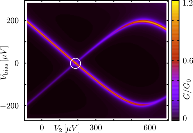
Figure 2: Andreev conductance measured from the left lead as a function of bias voltage and QD potential (measured relative to quarter filling) for the second dot. Changing the chemical potential allows to tune quasi-bound states to zero energy (white circle).

Second step: tuning the superconducting phases. We now set the phases of the induced pairing potentials $\Phi_{n}$ to constant. As explained in the previous section, this occurs when $\Delta_{n}$ and $t_{n}$ experience their maximal and minimal values. According to Eq. (3) this happens when the separation between the energy levels of the pair of dots subsection is maximal. Fig. 3 shows the evolution of these levels as a function of the phase difference between the two superconductors. The condition $\delta\Phi_{1}=0$ is then satisfied at the point where their separation is maximal.

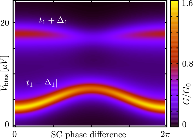
Figure 3: Conductance as a function of bias voltage and superconducting phase difference for a two-dot system. The two lowest energy levels are given by Eq. (3) of a two site Kitaev chain, as indicated. At the point where their separation is maximal (SC phase difference 0 in the plot), the phase difference $\delta\Phi_{n}$ of the induced superconducting gaps vanishes.

Third step: tuning the couplings. Finally we tune $t_{n}=\Delta_{n}$. This is achieved by varying $G_{\perp}$, while tracking the Andreev conductance peak corresponding to the $t_{n}-\Delta_{n}$ eigenvalue of the Kitaev chain we are emulating. After every change of $G_{\perp}$ we readjust $V_{n}$ in order to make sure that the condition $\varepsilon_{n}=0$ (or equivalently $V_{z}^{2}=\mu_{n}^{2}+\Delta_{n}^{2}$) is maintained. This is necessary because not just $\Delta_{n}$, but also $\mu_{n}$ depend on $G_{\perp}$. Therefore, successive changes of $G_{\perp}$ and $V_{n}$ are performed until the smallest bias peak is located at zero bias. The tuning steps of the first two dots are shown in Fig. 4. We repeat steps 2 and 3 for each pair of dots in the system.

Figure 4: Conductance as a function of bias voltage during simultaneous tuning of $G_{\perp}$ and $V_{n}$ for the first pair of dots. The three different plots represent the situation before (dotted line), at an intermediate stage (dashed line), and after (solid line) the tuning. The arrow indicates the evolution of the first peak upon tuning, and the number of successive changes of $G_{\perp}$ and $V_{n}$ are shown for each curve. By bringing the first peak to zero, the third tuning step is achieved.

Finally, having full all three conditions required for a robust topologically non-trivial phase, we probe the presence of localized Majorana bound state in the full three-dot system by measuring Andreev conductance (see Fig. 5). In this specific case, the height of the zero bias peak is approximately $1.85\,G_{0}$, signaling that the end states are well but not completely decoupled. Increasing the transparency of the QPC connecting the first dot to the lead brings this value to $G=1.98\,G_{0}$.

Figure 5: Conductance as a function of bias voltage for a system composed of three tuned quantum dots (dashed line). The zero bias peak signals the presence of Majorana bound states at the ends of the chain. The first and second excited states are consistent with those expected for a three-site Kitaev chain, namely $E_{1}=2t_{1}$ and $E_{2}=2t_{2}$ (vertical dashed lines), given the measured values of $t_{1}=\Delta_{1}$ and $t_{2}=\Delta_{2}$, obtained after finalizing the two dot tuning process. As described in the main text, after increasing the transparency of the lead QPC leads to a zero bias peak having a height $G=1.98G_{0}$ (solid line).

V Conclusion

In conclusion, we have demonstrated how to tune a linear array of quantum dots coupled to superconductors in presence of Zeeman field and spin-orbit coupling to resemble the Kitaev chain that hosts Majorana bound states at its ends. Furthermore, we have presented a detailed procedure by which the system is brought to the so-called “sweet spot” in parameter space, where the Majorana bound states are the most localized. This procedure involves varying the gates potentials and superconducting phases, as well as monitoring of the excitation spectrum of the system by means of resonant Andreev conductance.

We have tested our procedure using numerical simulations of a system of three QDs, defined in a 2DEG, and found that it works in systems with experimentally reachable parameters. It can be also applied to systems where quantum dots are defined by other means, for example formed in a one-dimensional InAs or InSb wire.

Appendix A System parameters in numerical simulations

In this section, we describe the parameters used throughout the numerical simulations. The quantum dots and quantum point contacts are modeled using a tight-binding model defined on a square lattice, with leads and superconductors taken as semi-infinite.

The characteristic length and energy scales of this system are the spin-orbit length $l_{\text{SO}}=\hbar^{2}/m\alpha$, and the spin-orbit energy $E_{\text{SO}}=m\alpha^{2}/\hbar^{2}$. We simulate an InAs system in which the effective electron mass is $m=0.015m_{e}$, where $m_{e}$ is the bare electron mass, taking values of $E_{\text{SO}}=1\,\text{K}=86\,\mu eV$ and $l_{\text{SO}}=250\,\text{nm}$.

We consider a setup composed of three quantum dots, like the one shown in Fig. 6. Each of the three dots has a length of $L_{\rm DOT}=208\,\text{nm}$ and a width $W_{\rm DOT}=104\,\text{nm}$. Quantum point contacts have a longitudinal dimension of $L_{\rm QPC}=42\,\text{nm}$, which is the same as the Fermi wavelength at quarter filling.

Figure 6: Geometry of the quantum dot chain. The quantum dots have a width $W_{\rm DOT}$ and length equal to $L_{\rm DOT}$. Quantum point contacts have a longitudinal size $L_{\rm QPC}$ and a transverse dimension equal to either $L_{\rm DOT}$ or $W_{\rm DOT}$. Leads are semi-infinite in the $x$ direction, and superconductors are modeled as semi-infinite systems in the $y$ direction.

The value of the hopping integral becomes $t=\hbar^{2}/(2ma^{2})=55.8\,\text{meV}$, with $a=7\,\text{nm}$. Disorder is introduced in the form of random uncorrelated onsite potential fluctuations, leading to a mean free path $l_{\text{mfp}}=218.8\,\text{nm}$. The system is placed in a perpendicular magnetic field characterized by a Zeeman splitting $V_{z}=336\,\mu\text{eV}$, which, given a $g$-factor of $35K/T$, corresponds to a magnetic field $B_{z}=111\,\text{mT}$. Each dot is additionally connected to a superconductor characterized by a pairing potential $|\Delta_{\text{SC}}|=0.86\,\text{meV}$.

The potential profile across a quantum point contact is given by

$$V_{\rm QPC}(x) = \frac{\widetilde{h}}{2}\left(2-\tanh\left(\frac{\widetilde{s}}{\widetilde{L}}\left(x+\frac{\widetilde{w}}{2}\right)\right)\right.$$ (13)

$$\left.+\tanh\left({\frac{\widetilde{s}}{\widetilde{L}}\left(x-\frac{\widetilde{w}}{2}\right)}\right)\right),$$

where $x\in[-\widetilde{L}/2,\widetilde{L}/2]$ is the transverse coordinate across the quantum point contact, $\widetilde{h}$ is the maximum height of $V_{\rm QPC}$, $\widetilde{s}$ fixes the slope at which the potential changes, and $\widetilde{w}$ is used to tune the QPC transparency. Two examples of potential profiles are shown in Fig. 7.

Figure 7: Potential profile $V_{\rm QPC}(x)$ across the transverse direction of a quantum point contact. For the maximum value of this potential, no states are available for quasiparticles in the 2DEG. The two curves show potential profiles for two different QPC transparencies, corresponding to $\widetilde{s}=17$ and $\widetilde{w}=87.4$, $39.5$ nm for the solid and dashed curves respectively.

Figure 8: Conductance of a quantum point contact as a function of $\widetilde{w}$ of Eq. (13), for a single QPC. The vertical lines indicate the values at which QPCs are set after tuning. The inter-dot QPCs are all set to the tunneling regime while the ones connecting the dots to the superconductors are set to higher transparencies.

References

- (1) J. Alicea, Rep. Prog. Phys. 75, 076501 (2012).
- (2) C. W. J. Beenakker, arXiv:1112.1950 (2011).
- (3) J. D. Sau, R. M. Lutchyn, S. Tewari, and S. Das Sarma, Phys. Rev. Lett. 104, 040502 (2010).
- (4) R. M. Lutchyn, J. D. Sau and S. Das Sarma, Phys. Rev. Lett. 105, 077001 (2010).
- (5) Y. Oreg, G. Refael and F. Von Oppen, Phys. Rev. Lett. 105, 177002 (2010)
- (6) V. Mourik, K. Zuo, S. M. Frolov, S. R. Plissard, E. P. A. M. Bakkers, and L. P. Kouwenhoven, Science 336, 1003 (2012).
- (7) M. T. Deng, C. L. Yu, G. Y. Huang, M. Larsson, P. Caroff, and H. Q. Xu, arXiv:1204.4130.
- (8) A. Das, Y. Ronen, Y. Most, Y. Oreg, M. Heiblum, and H. Shtrikman, arXiv:1205.7073.
- (9) L. P. Rokhinson, X. Liu, and J. K. Furdyna, arXiv:1204.4212 (2012).
- (10) C. J. Bolech and E. Demler, Phys. Rev. Lett. 98, 237002 (2007).
- (11) K. T. Law, P. A. Lee, and T. K. Ng, Phys. Rev. Lett. 103, 237001 (2009).
- (12) S. Sasaki, S. De Franceschi, J. M. Elzerman, W. G. van der Wiel, M. Eto, S. Tarucha, and L. P. Kouwenhoven, Nature 405, 764 (2000).
- (13) D. I. Pikulin, J. P. Dahlhaus, M. Wimmer, H. Schomerus, and C. W. J. Beenakker, arXiv:1206.6687.
- (14) K. Flensberg, Phys. Rev. B 82, 180516(R) (2010).
- (15) G. Kells, D. Meidan, and P. W. Brouwer, Phys. Rev. B 85, 060507(R) (2012).
- (16) S. Tewari, T. D. Stanescu, J. D. Sau, and S. Das Sarma, Phys. Rev. B 86, 024504 (2012).
- (17) F. Pientka, G. Kells, A. Romito, P. W. Brouwer, and F. von Oppen, arXiv:1206.0723.
- (18) J. Liu, A. C. Potter, K. T. Law, and P. A. Lee, arXiv:1206.1276.
- (19) P. W. Anderson, J. Phys. Chem. Solids 11, 26 (1959).
- (20) A. C. Potter and P. A. Lee, Phys. Rev. Lett. 105, 227003 (2010).
- (21) T. D. Stanescu, R. M. Lutchyn, and S. Das Sarma, Phys. Rev. B 84, 144522 (2011).
- (22) P. W. Brouwer, M. Duckheim, A. Romito and F. von Oppen, Phys. Rev. Lett. 107, 196804 (2011).
- (23) M.-T. Rieder, G. Kells, M. Duckheim, D. Meidan, and P. W. Brouwer, Phys. Rev. B 86, 125423 (2012).
- (24) M. Wimmer, A.R. Akhmerov, J.P. Dahlhaus, C.W.J. Beenakker, New J. Phys. 13, 053016 (2011).
- (25) A. Yu. Kitaev, Phys.-Usp. 44, 131 (2001).
- (26) J. D. Sau, S. Das Sarma, Nat. Comm. 3, 964 (2012).
- (27) J. Alicea, Y. Oreg, G. Refael, F. Von Oppen, M. P. A. Fisher, Nat. Phys. 7, 412 (2011).
- (28) J. D. Sau, D. J. Clarke, S. Tewari, Phys. Rev. B 84, 094505 (2011).
- (29) T.-P. Choy, J. M. Edge, A. R. Akhmerov, C. W. J. Beenakker, Phys. Rev. B 84, 195442 (2011).
- (30) M. Kjaergaard, K. Wölms, K. Flensberg, Phys. Rev. B 85, 020503(R) (2012).
- (31) B. Braunecker, G. I. Japaridze, J. Klinovaja, D. Loss, Phys. Rev. B 82, 045127 (2010).
- (32) Q.-F. Sun, J. Wang, H. Guo, Phys. Rev. B 71, 165310 (2005).
- (33) A. L. Shelankov, Zh. Eksp. Teor. Fiz., Pis’ma. 32, 2, 122-125 (1980).
- (34) G. E. Blonder, M. Tinkham, and T. M. Klapwijk, Phys. Rev. B 25, 4515 (1982).
- (35) H. Grabert and M. H. Devoret, Single Charge Tunneling: Coulomb Blockade Phenomena in Nanostructures (Plenum, New York, 1992)