Equilibrium disks, MRI mode excitation, and steady state turbulence in global accretion disk simulations.

Abstract

Global three dimensional magnetohydrodynamic (MHD) simulations of turbulent accretion disks are presented which start from fully equilibrium initial conditions in which the magnetic forces are accounted for and the induction equation is satisfied. The local linear theory of the magnetorotational instability (MRI) is used as a predictor of the growth of magnetic field perturbations in the global simulations. The linear growth estimates and global simulations diverge when non-linear motions - perhaps triggered by the onset of turbulence - upset the velocity perturbations used to excite the MRI. The saturated state is found to be independent of the initially excited MRI mode, showing that once the disk has expelled the initially net flux field and settled into quasi-periodic oscillations in the toroidal magnetic flux, the dynamo cycle regulates the global saturation stress level. Furthermore, time-averaged measures of converged turbulence, such as the ratio of magnetic energies, are found to be in agreement with previous works. In particular, the globally averaged stress normalized to the gas pressure, $\overline{<\alpha_{\rm P}>}=0.034$, with notably higher values achieved for simulations with higher azimuthal resolution. Supplementary tests are performed using different numerical algorithms and resolutions. Convergence with resolution during the initial linear MRI growth phase is found for $23-35~{}$cells per scaleheight (in the vertical direction).

1. Introduction

Accretion disks are ubiquitous in astrophysics and play an essential part in the formation of stars and galaxies. For accretion through a disk to be effective, angular momentum must be transported radially outwards, allowing material to move radially inwards. One means of achieving this is through viscous torques (Lynden-Bell & Pringle 1974), and considerable progress has been made using the phenomenological $\alpha$-viscosity introduced by Shakura & Sunyaev (1973) which assumes that viscosity is provided by turbulent stresses which scale with the gas pressure. However, despite its successes, the $\alpha$-viscosity model provides little physical insight into the mechanism(s) responsible for the turbulent stress.

Even prior to the work of Shakura & Sunyaev (1973), instabilities in magnetized rotating plasmas had been discovered by Velikhov (1959) and Chandrasekhar (1960). Yet, it was not until the seminal work of Balbus & Hawley (1991, 1998) that the so-called magnetorotational instability (MRI) received widespread attention as the agent responsible for the onset of accretion disk turbulence. Linear stability analysis has shown that the MRI will amplify a seed magnetic field indefinitely until confronted by the strong-field limit or the diffusion scale (Balbus & Hawley 1992; Terquem & Papaloizou 1996; Papaloizou & Terquem 1997). Non-linear stability analysis finds that growth of the magnetic field by the linear phase of the MRI is likely to be truncated by saturation resulting from secondary, or parasitic, instabilities (e.g. Goodman & Xu 1994; Pessah 2010). That saturation of the magnetic field occurs was clearly demonstrated by even the very first shearing box simulations (Brandenburg et al. 1995; Hawley et al. 1995; Stone et al. 1996).

Contemplating the next steps in magnetized disks studies is aided by summarising what we have already learned. For example, as mentioned above, it is clear that the magnetic field reaches saturation and that the resulting Maxwell stress dominates the angular momentum transport. In numerical simulations this necessitates high resolution to ensure that the fastest growing MRI modes are sufficiently well resolved (see, e.g., Sano et al. 2004; Fromang & Nelson 2006; Noble et al. 2010; Flock et al. 2011; Hawley et al. 2011). Related to this point is the importance of stratification, which introduces a characteristic length scale, removing the problem of non-convergence with simulation resolution encountered in unstratified simulations (Fromang & Papaloizou 2007; Lesur & Longaretti 2007; Simon et al. 2009; Guan et al. 2009; Davis et al. 2010; Sorathia et al. 2012). Stratification could also play a role in the dynamo process which sets the saturation stress (Brandenburg 2005; Vishniac 2009; Shi et al. 2010; Gressel 2010). However, the shearing box approximation used in a large number of numerical studies to-date has limitations (e.g. Regev & Umurhan 2008; Bodo et al. 2008, 2011), including the use of shearing-periodic boundary conditions in the radial direction, and/or periodic boundary conditions in the vertical direction. There boundary conditions artificially trap magnetic flux, assisting the maintenance of the turbulent dynamo and obscuring the dependence of the saturated state on resolution. This is supported by a comparison of periodic and open boundary conditions in global models by Fromang & Nelson (2006) where the former were found to assist the dynamo by preventing magnetic flux from being expelled from the domain. In this regard global models have the advantage of removing the unphysical influence of the shearing box boundary conditions, albeit at a much larger computational expense.

Other motivations for global models are the results from stability analyses of non-axisymmetric disturbances in magnetized accretion disks, where the most robust MRI modes are localized and the most robust buoyant (Parker) modes are global (Terquem & Papaloizou 1996; Papaloizou & Terquem 1997). Therefore, large radial extents are required to accommodate the more global modes, and in this regard there is a limit to the radial periodicity adopted in most shearing box simulations. These factors point to the need for high resolution, global, stratified disk simulations to further unravel the complexities of magnetorotational turbulence.

Of the global simulation studies that have been performed a large number of the findings from local models have been maintained or have persisted; the ratio of the Maxwell and Reynolds stress is $\sim 3$, and variations in toroidal magnetic field with time are suggestive of a dynamo cycle (Hawley 2000; Hawley & Krolik 2002; Fromang & Nelson 2006, 2009; Lyra et al. 2008; Sorathia et al. 2010, 2012; Flock et al. 2010, 2011, 2012; O’Neill et al. 2011; Hawley et al. 2011; Beckwith et al. 2011; Mignone et al. 2012; McKinney et al. 2012; Romanova et al. 2012). However, a large number of these simulations do not start from fully equilibrium initial conditions where the magnetic field is accounted for in the force balance and in the induction equation. Both local and global models started with poloidal fields which do not satisfy the induction equation show rapid disruption and re-arrangement of the disk (e.g. Miller & Stone 2000; Hawley 2000; Hawley et al. 2011). This introduces a transient phase where channel flows are fueled by rapid shearing of the poloidal field lines. As such, extended run times are required to ensure that transients have subsided. To our knowledge, no previous global simulations of the MRI in stratified disks have used a fully equilibrium initial disk (i.e. satisfying force balance and the induction equation).

We aim to explore the influence of magnetic fields on an accretion disk with global simulations. In this first paper we present equilibrium initial disk models with arbitrary radial density and temperature profiles. We then investigate the saturation (both locally and globally) of the growth of magnetic field perturbations. To this end we excite the MRI in global simulations using linear MRI calculations as a guide, and recover growth of magnetic field perturbations in agreement with estimates. In so doing we show that non-linear gas motions saturate the initial growth of the magnetic field and that at later times the turbulent state retains no knowledge of the initially excited MRI mode(s).

The plan of this paper is as follows: in § 2 we describe the equilibrium initial conditions and details of the numerical calculations and in § 3 we perform a linear perturbation analysis for the non-axisymmetric MRI. We present a suite of global magnetized disk simulations in § 4, which explore the effect of different MRI mode excitation and numerical algorithms. In § 5 we compare our results to previous work, and then close with conclusions in § 6.

2. The model

2.1. Simulation code

For our global disk simulations, we use a 3D spherical $(r,\theta,\phi)$ coordinate system with a domain which closely encapsulates the initial disk (e.g. Fromang & Nelson 2006), and we solve the time-dependent equations of ideal MHD using the PLUTO code (Mignone et al. 2007). We note that throughout this work we describe our results in terms of both spherical $(r,\theta,\phi)$ and/or cylindrical $(R,\phi,z)$ coordinates, with $R=r\sin\theta$ and $z=r\cos\theta$. The relevant equations for mass, momentum, energy conservation, and magnetic field induction are:

$$\frac{\partial\rho}{\partial t}+\nabla\cdot[\rho{\bf v}] = 0,$$ (1)

$$\frac{\partial\rho{\bf v}}{\partial t}+\nabla\cdot[\rho{\bf vv}-{\bf BB}+(P+\frac{1}{2}|{\bf B}|^{2}){\bf I}] = -\rho\nabla\Phi,$$ (2)

$$\frac{\partial E}{\partial t}+\nabla\cdot[(E+P){\bf v}-({\bf v\cdot B}){\bf B}] = -\rho{\bf v}\cdot\nabla\Phi-\rho\Lambda$$

$$\frac{\partial\bf B}{\partial t} = \nabla\times({\bf v\times B}).$$ (4)

Here $E=\rho\epsilon+\frac{1}{2}\rho|{\bf v}|^{2}+\frac{1}{2}|{\bf B}|^{2}$, is the total gas energy density, $\epsilon$ is the internal energy per unit mass, ${\bf v}$ is the gas velocity, $\rho$ is the mass density, and $P$ is the pressure. We use the ideal gas equation of state, $\rho\epsilon=P/(\gamma-1)$, where the adiabatic index $\gamma=5/3$. The adopted scalings for density, velocity, temperature, and length are, respectively,

$$\rho_{\rm scale} = 1.67\times 10^{-7}~{}{\rm gm~{}s^{-1}},$$

$$v_{0} = c,$$

$$T_{\rm scale} = \mu mc^{2}/k_{\rm B}=6.5\times 10^{12}~{}{\rm K},$$

$$l_{\rm scale} = 1.48\times 10^{13}~{}{\rm cm},$$

where $c$ is the speed of light, and the value of $l_{\rm scale}$ corresponds to the gravitational radius of a $10^{8}~{}{\rm M_{\odot}}$ black hole.

The gravitational potential, $\Phi$ of a central point mass (ignoring self-gravity of the disk), $\Phi$ is modelled using the pseudo-Newtonian potential introduced by Paczyńsky & Wiita (1980):

$$\Phi=\frac{-1}{r-2}.$$ (5)

Note that we take the gravitational radius (in scaled units), $r_{\rm g}=1$. The Schwarzschild radius, $r_{\rm s}=2$ for a spherical black hole and the innermost stable circular orbit (ISCO) lies at $r=6$. The $\Lambda$ term on the RHS of Eq (LABEL:eqn:energy) is an ad-hoc cooling term used to keep the scaleheight of the disk approximately constant throughout the simulations; without any explicit cooling in conjunction with an adiabatic equation of state, dissipation of magnetic and kinetic energy leads to an increase in gas pressure and, consequently, the disk scaleheight over time. The form of $\Lambda$ is particularly simple,

$$\Lambda=\frac{\rho}{(\gamma-1)}\frac{T(R,z)-T_{\rm 0}(R)}{2\pi R/v_{\phi}}$$ (6)

where $T_{0}(R)$ and $T(R,z)$ are the position dependent initial and current temperature, respectively, $v_{\phi}$ is the rotational velocity, and $R$ is the cylindrical radius. This cooling function drives the temperature distribution in the disk back towards the initial one over a timescale of an orbital period and is similar in its purpose to the cooling functions used by Shafee et al. (2008), Noble et al. (2010), and O’Neill et al. (2011). Note that we only apply cooling within $|z|<2H$, where $H$ is the scaleheight of the disk, allowing heating via dissipation to occur freely in the corona. Our choice of an orbital period for the cooling timescale is somewhat arbitrary but is chosen as it represents a characteristic timescale for the disk.

The PLUTO code was configured to use the five-wave HLLD Riemann solver of Miyoshi & Kusano (2005), piece-wise parabolic reconstruction (PPM - Colella & Woodward 1984), and second-order Runge-Kutta time-stepping. In order to maintain the ${\bf\nabla\cdot B}=0$ constraint for the magnetic field we use the upwind Constrained Transport (UCT) scheme of Gardiner & Stone (2008). Such a configuration has been shown to be effective in recovering the linear growth rates of the axisymmetric MRI by Flock et al. (2010). In § 4.4 we test a number of different numerical setups: order of reconstruction, slope limiters, and simulation resolution. However, in all of the other global simulations presented in § 4 we use reconstruction on characteristic variables (e.g. Rider et al. 2007). A Courant-Friedrichs-Lewy (CFL) value of 0.35 was used for all simulations.

The grid used for the global simulations is uniform in the $r$ and $\phi$ directions and extends from $r=4-34$ and $\phi=0-\pi/2$. In the $\theta$ direction we use a graded mesh which places slightly more than half of the cells within $|z|\leq 2H$ of the disk mid-plane with a uniform $\Delta\theta$, where $H$ is the thermal disk scaleheight, and the remainder of the cells on a stretched mesh between $2H<|z|<5H$. For example, for simulation gbl-$m10$ the 256 cells in the $\theta$ direction are distributed so that 140 cells are uniformly spaced between $2H<|z|<5H$. The respective grid resolutions and number of cells per scaleheight for the three global simulations are noted in Table 2. The grid cell aspect ratio at the mid-plane of the disk and at a radius of $r=18.5$ (i.e. the disk midpoint) are $r\Delta\theta:\Delta r:r\Delta\phi=1:1.4:8.6$ and $1:1.6:2.5$ for models gbl-$m10$ and gbl-$m10+$, respectively. The $r$ and $\theta$ boundary conditions depend on whether the cell adjacent to the boundary contains $>1\%$ disk material - which we determine using a tracer variable. If this constraint is satisfied we use outflow boundary conditions on all hydrodynamic variables except $v_{\phi}$ which is determined from a zero-shear boundary condition (i.e. $d\Omega/dr=0$) and the normal velocity, for which we enforce zero inflow. If the condition on disk material at the boundary is not satisfied we use outflow boundary conditions on hydrodynamic variables with the limit that the values must lie between the floor values and the initial conditions for the background atmosphere - we find this choice to be useful in setting up a steady background inflow during the early stages of the simulation before material initially in the disk evolves to fill the domain. For the magnetic field we use zero gradient boundary conditions on the tangential field components and allow the UCT algorithm to calculate the normal component so as to satisfy the divergence free constraint, with the exception that at the inner radial boundary we enforce a negative magnetic stress condition (e.g. Stone & Pringle 2001). A periodic boundary condition is used in the $\phi$ direction. Finally, we use floor density and pressure values which scale linearly with radius and have values at the outer radial boundary of $10^{-4}$ and $5\times 10^{-9}$, respectively.

2.2. Initial conditions

Motivated by the fact that magnetorotationally turbulent disks are dominated by toroidal field, we start from an analytic equilibrium disk with a purely toroidal magnetic field. The disk equilibrium is derived in axisymmetric cylindrical coordinates $(R,z)$; further details can be found in Appendix A along with alternative disk solutions which may be of use in future work. In the following we briefly summarise the equations for the isothermal in height, $T=T(R)$, constant ratio of gas-to-magnetic pressure, $\beta=2P/|B|^{2}\equiv 2P/B_{\phi}^{2}$, net magnetic flux disk adopted for the simulations presented in this paper. The choice of temperature and magnetic field lead to a density distribution, in scaled units,

$$\rho(R,z)=\rho(R,0)\exp\left(\frac{-\{\Phi(R,z)-\Phi(R,0)\}}{T(R)}\frac{\beta}{1+\beta}\right),$$ (7)

where the pressure, $P=\rho T$. For the radial profiles $\rho(R,0)$ and $T(R)$ we use simple functions inspired by the Shakura & Sunyaev (1973) disk model, except with an additional truncation of the density profile at a specified outer radius:

$$\rho(R,0) = \rho_{0}f(R,R_{0},R_{\rm out})\left(\frac{R}{R_{0}}\right)^{\epsilon},$$ (8)

$$T(R) = T_{\rm 0}\left(\frac{R}{R_{0}}\right)^{\chi},$$ (9)

where $\rho_{0}$ sets the density scale, $R_{0}$ and $R_{\rm out}$ are the radius of the inner and outer disk edge, respectively, $f(R,R_{0},R_{\rm out})$ is a tapering function and is described in Appendix A, and $\epsilon$ and $\chi$ set the slope of the density and temperature profiles, respectively. In all of the global simulations $R_{0}=7$, $R_{\rm out}=30$, $\rho_{0}=10$, $T_{0}=4.5\times 10^{-4}$, $\epsilon=-33/20$, and $\chi=-9/10$ (consistent with the radial scaling in the gas pressure and Thomson-scattering opacity dominated region from Shakura & Sunyaev 1973), producing disks with an aspect ratio, $H/R=0.05$. The rotational velocity of the disk is close to Keplerian, with a minor modification due to the gas and magnetic pressure gradients,

$$v_{\phi}^{2}(R,z)=v_{\phi}^{2}(R,0)+\{\Phi(R,z)-\Phi(R,0)\}\frac{R}{T}\frac{dT}{dR},$$ (10)

where,

$$v_{\phi}^{2}(R,0)=R\frac{\partial\Phi(R,0)}{\partial R}+\frac{2T}{\beta}+$$

$$\left(\frac{1+\beta}{\beta}\right)\left(\frac{RT}{\rho(R,0)}\frac{\partial\rho(R,0)}{\partial R}+R\frac{dT}{dR}\right).$$ (11)

One advantage using such an equilibrium disk is that one begins with a disk that is close to the expected scale height and density. An isothermal disk, for example, has a scale height that is proportional to $R^{3/2}$.

Finally, the region outside of the disk is set to be an initially stationary, spherically symmetric, hydrostatic atmosphere with a temperature and density given by,

$$T_{\rm atm}(r) = -\frac{\Phi}{2},$$ (12)

$$\rho_{\rm atm}(r) = \rho_{\rm atm}(r_{\rm ref})\left(\frac{\Phi(r)}{\Phi(r_{\rm ref})}\right),$$ (13)

where $\rho_{\rm atm}=4\times 10^{-5}\rho_{0}$ and $r_{\rm ref}$ is a reference radius which we take to be $R_{\rm max}$, the radius of peak disk density (see Appendix A). The transition between the disk and background atmosphere occurs where their total pressures balance.

As an example, model gbl-$m10$ corresponds to a disk with a peak density of $1.67\times 10^{-7}~{}{\rm gm~{}s^{-1}}$ and a peak temperature of $2.9\times 10^{9}~{}{\rm K}$.

2.3. Diagnostics

Turbulence is by its very nature chaotic. Therefore, averaged quantities are particularly useful diagnostics. In this section we describe how we calculate averages, and define the variables used to analyse the simulations.

To compute shell-averaged values (denoted by curly brackets) of a variable $q$ at a radius $r$ we average in the $\theta$ and $\phi$ directions via,

$$\{q\}=\frac{\int qr^{2}\sin\theta d\theta d\phi}{\int r^{2}\sin\theta d\theta d\phi}.$$ (14)

Similarly, we calculate a horizontally averaged value (denoted by square brackets) as,

$$[q]=\frac{\int qr\sin\theta drd\phi}{\int r\sin\theta drd\phi}$$ (15)

To attain a volume-averaged value (denoted by angled brackets) we integrate over the radial profile of shell-averaged values and normalize by the radial extent,

$$<q>=\frac{\int\{q\}dr}{\int dr}$$ (16)

Time averages receive an overbar, such that a volume and time averaged quantity would read $\overline{<q>}$. (Note that density-weighted averages are computed, but only for hydrodynamical variables.) For the analysis presented in § 4 we restrict the integration over $r$ and $\theta$ to the range $10<r<30$ and in $\pi/2-\theta_{2H/R}<\theta<\pi/2+\theta_{2H/R}$, where $\theta_{2H/R}=\tan^{-1}(2H/R)$. We define this region as the “disk body” and limit the integration over this region to allow comparison against recent global (e.g. Fromang & Nelson 2006; Beckwith et al. 2011; Sorathia et al. 2010; Flock et al. 2011, 2012; Hawley et al. 2011; Sorathia et al. 2012) and large local simulations (e.g. Guan & Gammie 2011; Simon et al. 2012).

In order to keep a track of the fluctuations in the scaleheight of the disk during the simulation - which results from the interplay between adiabatic heating and our cooling function - a density-weighted average disk scaleheight is computed, where we take $H/R=c_{\rm s}/v_{\phi}$ (where $c_{\rm s}$ is the sound speed), then perform a density-weighted shell-average followed by a radial averaging to acquire a volume averaged value, $<H/R>$.

For accretion to occur, angular momentum must be transported radially outwards by turbulent stresses, and a major focus of numerical simulations is quantifying the stress. To this end, we define the perturbed flow velocity as $\delta v_{\rm i}=v_{\rm i}-\int v_{\rm i}r\sin\theta d\phi/\int r\sin\theta d\phi$ with ${\rm i}={\rm R},\phi$, and compute the $R-\phi$ component of the combined Reynolds and Maxwell stress,

$$W_{R\phi}=\rho\delta v_{\rm R}\delta v_{\phi}-B_{\rm R}B_{\phi},$$ (17)

which is normalized by the gas pressure to acquire,

$$\{\alpha_{\rm P}\}=\frac{\{W_{R\phi}\}}{\{P\}}.$$ (18)

Furthermore, we calculate the $R-\phi$ component of the Maxwell stress normalized by the magnetic pressure,

$$\{\alpha_{\rm M}\}=\frac{-2\{B_{\rm R}B_{\phi}\}}{\{|B|^{2}\}}.$$ (19)

To examine the operation of dynamo activity in the disk we compute the toroidal magnetic flux, which is defined as,

$$\Psi_{\phi}(\phi)=\int\int B_{\phi}(\phi)r\sin\theta drd\theta.$$ (20)

The ability of the simulations to resolve the fastest growing MRI modes is quantified in the same fashion as Noble et al. (2010) and Hawley et al. (2011). The wavelength of the fastest growing MRI modes with respect to the grid resolution in the $z$ and $\phi$ directions are, respectively,

$$Q_{\rm z}=\frac{\lambda_{\rm MRI-z}}{\Delta z}=\sqrt{\frac{16}{15}}\frac{2\pi|v_{Az}|r\sin\theta}{v_{\phi}\Delta z},$$ (21)

and,

$$Q_{\phi}=\frac{\lambda_{\rm MRI-\phi}}{R\Delta\phi}=\frac{2\pi|v_{A\phi}|}{\Delta\phi},$$ (22)

where $v_{\rm Az}$ and $v_{\rm A\phi}$ are the vertical and azimuthal Alfvén speeds, respectively, $\Delta\theta$ and $\Delta\phi$ are the cell sizes in the $\theta$ and $\phi$ directions, respectively, and $\Delta z=\sqrt{(r\sin\theta\Delta\theta)^{2}+(\Delta r\cos\theta)^{2}}$ is the corresponding cell size in the $z$ direction. We define a single valued measure of resolvability as the fraction of cells in the disk body ($|z|<2H$) that have $Q>8$ (e.g. Sorathia et al. 2012),

$$N_{\rm i}=\frac{\Sigma C(Q_{\rm i}>8)}{\Sigma C}$$ (23)

where ${\rm i}=z,\phi$ and $C$ represents a cell. The principal aim of calculating $N_{\rm z}$ and $N_{\phi}$ is to quantify how well resolved the turbulent state is in a simulation, and consequently whether global simulations are approaching the region of convergence found from shearing box simulations (Hawley et al. 2011).

2.4. Fourier analysis

To allow a direct comparison between the growth of MRI modes estimated from a linear perturbation analysis (§ 3) and the results of global simulations (§ 4) we analyse the growth of magnetic field perturbations in Fourier space. The procedure we follow is to remap the disk body (which we define in § 2.3) to a cylindrical mesh with uniform cell spacing in all directions, and a sufficiently fine resolution to ensure that the smallest cells from the spherical simulation grid are sampled. We then perform a 3D Fourier Transform of the data on the cylindrical grid. A detailed description of the cylindrical Fourier transform can be found in Appendix B.

3. Exciting the MRI

Given that our global simulations commence with an equilibrium disk the MRI requires a seed perturbation to excite the growth of the magnetic field and development of turbulence. For this purpose we have chosen to excite a specific Fourier mode of the MRI using poloidal velocity perturbations. In the following we present perturbation calculations for the local, linear, non-axisymmetric MRI, the results of which are used in § 4 to elucidate the evolution of magnetic field perturbations in global numerical simulations.

Table 1Parameters used for the linear MRI growth calculations

Model	$\beta$	$m$	$k_{\rm z}$	$k_{\rm R}$	$\left(\frac{{\bf k\cdot v_{\rm A}}}{\Omega}\right)^{2}$	$\delta v_{0}/c_{\rm s}$
lin-$m10$	20	10	5	2.5	0.03	0.1
lin-$m10$-$\beta$100	100	10	5	2.5	0.006	0.1
lin-$m10$-$\beta$300	300	10	5	2.5	0.002	0.1
lin-$m10$-$\beta 300s$	300	10	5	2.5	0.002	0.3
lin-$m40$	20	40	80	40	0.45	0.1

3.1. Linear MRI growth models

Studies of the linear, non-axisymmetric MRI in weakly magnetized disks have been examined by a number of authors (Balbus & Hawley 1992; Terquem & Papaloizou 1996; Papaloizou & Terquem 1997). Balbus & Hawley (1992)’s local study showed that even if the seed magnetic field is purely toroidal then the instability is still present, albeit with growth rates roughly an order of magnitude lower than those found for initially poloidal fields (Balbus & Hawley 1991). This result was supported by growth timescales approaching an orbital period (for certain parameters) in more-global calculations by Terquem & Papaloizou (1996) where radial gradients were preserved. Furthermore, these authors found that in the $k_{\rm z}/k_{\rm R}\ll 1$ limit - the primary domain of the MRI - instabilities become increasingly localized with time. On the other hand, in the $k_{\rm R}/k_{\rm z}\ll 1$ limit the Parker instability dominates. In fact, even in the presence of dissipation, MRI modes continue to become increasingly localized over time due to the time dependence of the radial wavenumber (Papaloizou & Terquem 1997). Common to these studies is the finding that the non-axisymmetric MRI acts as a mechanism for the transient amplification of seed magnetic/velocity field perturbations by many orders of magnitude over tens of orbits. One question is, how well does this immense field amplification carry through to global, fully non-linear simulations? To answer this one needs an estimate of the linear growth. In this regard our analysis of the non-axisymmetric MRI in this paper is complementary to studies of the axisymmetric MRI in previous simulations (e.g. Hawley & Balbus 1991; Flock et al. 2010).

To construct our prediction for the global simulations we utilize the linear MRI model of Balbus & Hawley (1992). (The perturbation analysis used to quantify the linear MRI growth is performed in cylindrical coordinates ($R,\phi,z$), whereas the global models presented in § 4 are performed in spherical coordinates ($r,\theta,\phi$).) In brief, Balbus & Hawley perform a linear stability analysis of a local patch of a disk using the shearing-sheet approximation (Goldreich & Lynden-Bell 1965) where the perturbations are assumed to have a spatial dependence $\exp[i(k_{\rm R}R+m\phi+k_{\rm z}z)]$. The equations for the evolution of the magnetic field perturbations form a pair of coupled second-order ordinary differential equations. We let $N$ be the Brunt-Väisälä frequency, which for the equilibrium disk described in § 2.2 is,

$$N^{2}=\frac{2}{5}\frac{1}{T}\left(\frac{\beta}{1+\beta}\right)^{2}\left(\frac{z}{R}\right)^{2}\frac{1}{(r-2)^{4}},$$ (24)

and define an independent time variable,

$$\tau = k_{\rm R}(t)R=k_{\rm R}(t=0)R-m\frac{d\Omega}{d\ln R}t,$$ (25)

$$k^{2} = k^{2}_{\rm R}+\frac{m^{2}}{R^{2}}+k^{2}_{\rm z}.$$ (26)

Replacing the angular velocity with that due to a Paczynski-Wiita potential in the thin disk limit (i.e. $H/R\ll 1$), $\Omega^{2}=1/R^{2}(R-2)$, the equations describing linear perturbations are,

$$\frac{d^{2}\delta B_{\rm z}}{d\tau^{2}}=\frac{2k_{\rm z}}{Rk^{2}(3R-2)}\left(\frac{2\tau^{2}}{m^{2}}(R-2)-R-2\right)\frac{d\delta B_{\rm R}}{d\tau}$$

$$-\frac{4}{m^{2}}\left(\frac{R-2}{3R-2}\right)^{2}\delta B_{\rm z}\left[\frac{({\bf k\cdot v_{\rm A}})^{2}}{\Omega^{2}}+\left(\frac{k^{2}-k_{\rm z}^{2}}{k^{2}}\right)\frac{N^{2}}{\Omega^{2}}\right]$$

$$+\frac{4k_{\rm z}\tau}{k^{2}m^{2}}\left(\frac{R-2}{3R-2}\right)\tau\frac{d\delta B_{\rm z}}{d\tau},$$

(27)

$$\frac{d^{2}\delta B_{\rm R}}{d\tau^{2}}=-\frac{4}{m^{2}}\left(1-\frac{k_{\rm R}^{2}}{k^{2}}\right)\frac{R-2}{3R-2}Rk_{\rm z}\frac{d\delta B_{\rm z}}{d\tau}$$

$$+\frac{2}{R^{2}k^{2}}\frac{R-2}{3R-2}\left[\frac{2}{m^{2}}(\tau^{2}-R^{2}k^{2})+\frac{R+2}{R-2}\right]\tau\frac{d\delta B_{\rm R}}{d\tau}$$

$$-\frac{4}{m^{2}}\left(\frac{R-2}{3R-2}\right)^{2}\left[\frac{({\bf k\cdot v_{\rm A}})^{2}}{\Omega^{2}}\delta B_{\rm R}-\frac{k_{\rm z}}{Rk^{2}}\frac{N^{2}}{\Omega^{2}}\tau\delta B_{\rm z}\right]$$

(28)

where $\delta B_{\rm z}$ and $\delta B_{\rm R}$ are the vertical and radial magnetic field perturbations.

The time dependence of $k_{\rm R}$ in Eq (25) is a consequence of the radial wavenumber being sheared. Therefore, within the framework of the Balbus & Hawley (1992) analysis the radial wavenumber can grow indefinitely so that radial disturbances can evolve to arbitrarily small spatial extent. Clearly, when we come to making a comparison against our global simulations, this will not be the case due to finite numerical resolution.

The magnetic field perturbations are related through the divergence-free constraint,

$${\bf k\cdot\delta B}=k_{\rm R}\delta B_{\rm R}+\frac{m}{R}\delta B_{\phi}+k_{\rm z}\delta B_{\rm z}=0.$$ (29)

The unperturbed magnetic field topology only enters through ${\bf k\cdot v_{\rm A}}$. For our initially purely toroidal magnetic field one finds,

$$\left(\frac{{\bf k\cdot v_{\rm A}}}{\Omega}\right)^{2}=\frac{2(R-2)m^{2}T}{\beta},$$ (30)

To initiate the MRI we use the $R$ and $z$ components of the linearized induction equation,

$$\frac{d\delta B_{\rm R}}{dt}=i({\bf k\cdot B})\delta v_{\rm R},$$ (31)

and,

$$\frac{d\delta B_{\rm z}}{dt}=i({\bf k\cdot B})\delta v_{\rm z},$$ (32)

where $\delta v_{\rm R}$ and $\delta v_{\rm z}$ are the poloidal velocity perturbations (with the imaginary part of $\delta v$ corresponding to the real part of $d\delta B/dt$). For the perturbations in the $z$-components in both the linear MRI and global calculations we use a waveform,

$$\delta v_{\rm z}=\delta v_{\rm 0}\cos(k_{\rm R}R+m\phi+k_{\rm z}z),$$ (33)

which, on substitution into Eq (32), and with the conversion between real and imaginary parts accounted for by a phase shift in the trigonometric term, leads to,

$$\frac{d\delta B_{\rm z}}{dt}=\delta v_{\rm 0}\frac{2B_{\phi}}{v_{\phi}}\frac{R-2}{3R-2}\sin(k_{\rm R}R+m\phi+k_{\rm z}z),$$ (34)

where $\delta v_{\rm 0}$ is the amplitude of the initial velocity perturbations. An equivalent treatment to Eq (34) is used for the perturbations in the $R$-components with the difference that we make use of the incompressibility condition, ${\bf k\cdot\delta v}=0$, and set,

$$\delta v_{\rm R}=\delta v_{\rm 0}\frac{k_{\rm z}}{k_{\rm R}}\cos(k_{\rm R}R+m\phi+k_{\rm z}z),$$ (35)

The remaining parameters used in the calculations are summarised in Table 1.

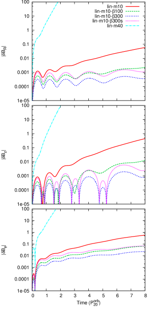
Figure 1.— The evolution of magnetic field perturbations from linear MRI growth calculations showing successful magnetic field amplification. From top to bottom: $\delta B_{\rm R},\delta B_{\rm z}$, and $\delta B_{\phi}$. The parameters used in these calculations are provided in Table 1.

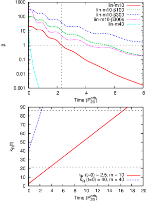
Figure 2.— (Top): The plasma-$\beta$ calculated from the linear MRI growth calculations - see Table 1 for the list of models and parameter values pertaining to each calculation. The vertical line indicates when model lin-$m10$ reaches $\beta=1$. (Bottom): The time-dependent radial wavenumber. The red and blue lines corresponds to models lin-$m10$ and lin-$m40$, respectively. The horizontal lines indicate the $k_{\rm R}$ values at the Nyquist limit for the global simulations gbl-$m10$ and gbl-$m10$-lllr (see Tables 3 and 2 and § 4).

Our first calculation, model lin-$m10$, uses a $\beta=20$ magnetic field and wavenumbers for the excited MRI mode of $m=10$, $k_{\rm z}=5$, and $k_{\rm R}=2.5$. These wavenumbers are chosen to ensure sufficient resolution in the global simulations and we leave a more detailed discussion to § 4. The amplitude of the initial velocity perturbations, $\delta v_{0}$, is set to $0.1~{}c_{\rm s}$, where $c_{\rm s}$ ($=\sqrt{T}$) is the sound speed. Since we intend to use these calculations as a guide for our global simulations, we use the equilibrium disk model described in § 2.2 to choose the input density and temperature. Calculations are performed at a cylindrical radius, $R=20$, and at the disk mid-plane where $N^{2}=0$ (see Eq (24)). From Eq (9) the disk temperature, $T=1.75\times 10^{-4}$, and the density, $\rho=0.46$. The initial components of $\delta{\bf B}$ are set to zero, so too is the initial azimuthal velocity perturbation, $\delta v_{\phi}$ - the poloidal velocity perturbations seed the instability through the $d\delta B/dt$ terms. To integrate Eqs (27) and (28) we use an adaptive stepsize, 4th-order, explicit Runge-Kutta method (Press et al. 1986). As Fig. 1 shows, the magnetic field perturbations grow extremely rapidly over the first few $P^{\rm orb}_{\rm 20}$ with noticeable oscillations, where $P^{\rm orb}_{\rm j}$ is the radially dependent orbital period of the disk at cylindrical radius j. The upper panel of Fig. 2 shows the effective $\beta$ for the MRI mode - the time required for the magnetic field to grow to $\beta=1$ is only a few orbital periods for model lin-$m10$. Evaluating the approximate growth rate, $\omega$ of the magnetic energy, $\beta^{-1}$ (as the gas pressure remains constant) via $\beta^{-1}=\beta^{-1}_{0}\exp(\omega t)$, we find an average growth rate over the first six orbits, $\overline{\omega}=0.14~{}\Omega$. Applying the same approach to $\delta B_{\rm R}$ we find $\overline{\omega}=0.09\Omega$. This is consistent with the findings of Terquem & Papaloizou (1996) but is roughly an order of magnitude larger than values of a few percent of the orbital frequency quoted in general for the development of the non-axisymmetric MRI by Balbus & Hawley (1992). Keeping all parameters fixed and then varying the initial magnetic field strength, one sees from models lin-$m10$-$\beta$100 and lin-$m10$-$\beta$300 the trend that the growth rate of $\delta{\bf B}$ decreases with increasing initial $\beta$. In model lin-$m10$-$\beta 300s$ the size of the initial velocity perturbations is increased to $\delta v_{0}=0.3~{}c_{\rm s}$ with the result that over the very first few orbits the growth of $\delta B$’s becomes very similar to that of a stronger initial field strength excited by smaller velocity perturbations. For a higher wavenumber perturbation the rate of initial growth increases, as evidenced by model lin-$m40$ (see Figs. 1 and 2). Evaluating the approximate growth rate of the magnetic field energy and $\delta B_{\rm R}$ for model lin-$m40$ gives, $\overline{\omega}=0.68~{}\Omega$ and $0.25\Omega$, respectively. From these results one may predict that the development of $\delta{\bf B}$ in simulations will depend on the initial field strength and/or the wavenumber of the excited mode(s). In § 4.3 we examine if this result holds true in global simulations.

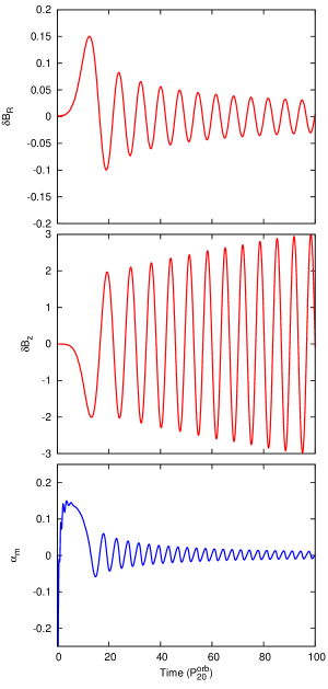
Figure 3.— Evolution of $\delta B_{\rm R}$ (upper), $\delta B_{\rm z}$ (middle), and $\alpha_{\rm m}$ (lower) as a function of time in model lin-$m10$ over a longer time duration than shown in Fig. 1.

Balbus & Hawley (1992) discuss the parameter $({\bf k\cdot v_{\rm A}})^{2}/\Omega^{2}$ and attribute to it an important role in the ability of the MRI to successfully amplify the seed field. They find that for $({\bf k\cdot v_{\rm A}})^{2}/\Omega^{2}\mathrel{\hbox to0.0pt{\lower 3.0pt\hbox{$\sim$}\hss}\raise 2.0pt\hbox{$>$}}2.9$ the instability is stabilized and magnetic field oscillations are damped. For the models shown in Fig. 1, this parameter is much less than unity. From Eq (30) for $({\bf k\cdot v_{\rm A}})^{2}/\Omega^{2}$ one can see that to increase the value of this variable one can either decrease $\beta$ - which increases the tension along field lines - or employ higher azimuthal wavenumbers, $m$. The latter has the side-effect of increasing the growth rate of $k_{\rm R}$ and causing tight wave crest wrapping, both of which lead to a more rapid stabilization of the radial disturbances. However, we find that irrespective of the value of $({\bf k\cdot v_{\rm A}})^{2}/\Omega^{2}$, which is $0.03$ for lin-$m10$ (Table 1), the perturbation in the magnetic field ultimately decays. This is shown in Fig 3 (upper and middle panels) where the lin-$m10$ calculation is plotted for a longer time duration. Despite continuing growth in $\delta B_{\rm z}$, there is decay in $\delta B_{\rm R}$, which is a consequence of the increase of $k_{\rm R}(t)$ combined with the divergence-free constraint (Eq (29)). The ratio of the Maxwell stress to magnetic pressure ($\alpha_{\rm m}$) predicted from the linear MRI growth calculations is shown in the lower panel of Fig. 3, where we define,

$$\alpha_{\rm m}=\frac{2\delta B_{\rm R}(\delta B_{\phi}+B_{\phi})}{B^{2}},B^{2}=B_{\phi}^{2}+\delta B_{\phi}^{2}+\delta B_{\rm R}^{2}+\delta B_{\rm z}^{2}.$$ (36)

Clearly, considering that $\alpha_{\rm m}$, or to be more exact

$<\alpha_{\rm M}>$ (its global analogue - see Eq (19)), is a commonly used diagnostic in numerical simulations (Hawley et al. 1995). Under the action of the linear MRI alone $<\alpha_{\rm M}>$ would never reach a steady value. This ultimate decay of linear MRI disturbances is consistent with Terquem & Papaloizou (1996)’s finding of transient instability growth in a number of numerical tests, in which $k_{\rm z}>k_{\rm R}$ initially. Shear causes $k_{\rm R}$ to grow but once $k_{\rm R}>k_{\rm z}$ growth halts.

The ultimate decay of linear MRI modes has significance for global models because the maintenance of dynamo action requires all components of the field to be sufficiently strong. This highlights the need for an additional mechanism, other than the linear MRI growth, to replenish $\delta B_{\rm R}$ (e.g. parasitic instabilities - Goodman & Xu 1994; Parker instability - Tout & Pringle 1992, Vishniac 2009; dynamo action in the steady-state turbulence Brandenburg et al. 1995, Hawley et al. 1996).

The linear MRI growth calculations act as a check on our global simulations, principally to examine whether our setup recovers the growth rates of the linear MRI accurately. However, there is a limit to the time interval when we can confidently make a comparison between the linear growth models and global simulations. Firstly, the analysis of Balbus & Hawley (1992) adopts the Boussinesq approximation which becomes invalid when the azimuthal magnetic field becomes super-thermal. The upper panel of Fig. 2 shows that this limit is reached in approximately 2.3 orbits for lin-$m10$ and 0.1 orbits for lin-$m40$. Secondly, $k_{\rm R}(t)$ can grow indefinitely in the linear growth models, yet this is not the case for our global simulations which are restricted by finite numerical resolution. Taking the Nyquist limit to be 2 grid cells, and considering, for example, the resolution of model gbl-$m10$, the maximum resolvable radial wavenumber is $k_{\rm R-Nyquist}=86$. This limit is reached after $\sim 16.5$ and 2.3 orbits for models lin-$m10$ and lin-$40$, respectively (lower panel of Fig. 2). Therefore, choosing to excite a higher wavenumber MRI mode limits the time interval where comparisons can be made against linear perturbation theory, and this is one reason why we choose to excite a lower wavenumber mode ($m=10$) in the global simulations.

Table 2Global simulations and the corresponding linear growth rate.

Model	Resolution	Reconstruction	Limiter	$n_{\rm r}/H$	$n_{\theta}/H$	$n_{\phi}/H$	$\omega_{\rm approx}$
	($n_{\rm r}\times n_{\theta}\times n_{\phi}$)			($10<r<30$)	($|z|<2H$)		($\Omega(R=20)$)
lin-$m10$	$-$	$-$	$-$	$-$	$-$	$-$	0.09 $\pm$ 0.01
gbl-$m10$	$768\times 256\times 128$	Parabolic	Char	18-77	35	4	0.15 $\pm$ 0.03
gbl-$m10+$	$512\times 170\times 320$	Parabolic	Char	12-51	27	12.5	0.11 $\pm$ 0.02
gbl-rand	$512\times 170\times 320$	Parabolic	Char	12-51	27	12.5	0.15 $\pm$ 0.04
gbl-$m10$-lin	$768\times 256\times 128$	Linear	Char	18-77	35	4	0.16 $\pm$ 0.03
gbl-$m10$-cw	$768\times 256\times 128$	Parabolic	CW84	18-77	35	4	0.13 $\pm$ 0.02
gbl-$m10$-cs	$768\times 256\times 128$	Parabolic	CS08	18-77	35	4	0.14 $\pm$ 0.02
gbl-$m10$-hr	$896\times 300\times 150$	Parabolic	Char	21-90	41	5	0.16 $\pm$ 0.04
gbl-$m10$-lr	$512\times 170\times 96$	Parabolic	Char	12-51	23	3	0.13 $\pm$ 0.03
gbl-$m10$-llr	$342\times 112\times 64$	Parabolic	Char	8-34	15	2	0.09 $\pm$ 0.04
gbl-$m10$-lllr	$192\times 64\times 32$	Parabolic	Char	5-19	9	1	0.05 $\pm$ 0.03

Table 3Time averaged quantities from the global simulations..

Model	$m$	$k_{\rm z}$	$k_{\rm R}$	$\frac{\delta v_{0}}{c_{\rm s}}$	$\delta t_{\rm av}$a	$\overline{N_{\rm z}}$	$\overline{N_{\phi}}$	$\overline{\frac{<B_{\rm R}^{2}>}{<B_{\phi}^{2}>}}$	$\overline{\frac{<B_{\rm z}^{2}>}{<B_{\rm R}^{2}>}}$	$\overline{\frac{<B_{\rm z}^{2}>}{<B_{\phi}^{2}>}}$	$\overline{<\alpha_{\rm P}>}$	$\overline{<\alpha_{\rm M}>}$	$\overline{<\beta>}$b
gbl-$m10$	10	5	2.5	0.1	10-28	0.32	0.33	0.071	0.25	0.018	0.017	0.31	32
gbl-$m10+$	10	5	2.5	0.001	12-26	0.45	0.75	0.12	0.29	0.036	0.034	0.41	17
gbl-rand	$-$	$-$	$-$	0.001	16-26	0.45	0.75	0.13	0.30	0.037	0.034	0.41	17

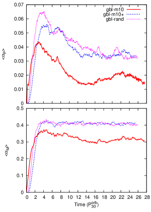
Figure 4.— The evolution of $<\alpha_{\rm P}>$ (upper) and $<\alpha_{\rm M}>$ (lower) in the global models as a function of time in units of the orbital period at $R=30$. See Table 3 for a list of the models and time averaged values.

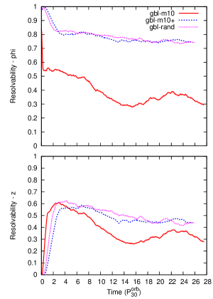
Figure 5.— Resolvability of the MRI in the $\phi$ direction (upper) and $z$ direction (lower) in models gbl-$m10$, gbl-$m10+$, and gbl-rand. For a definition of the resolvability see Eq (23) and § 2.3.

Figure 6.— Density-weighted and volume averaged scaleheight of the disk, $<H/R>$ as a function of time in models gbl-$m10$ (solid line) and gbl-$m10+$ (dashed line).

4. Global models

In this section we describe the results of global simulations using the initial conditions and simulation setup described in § 2. The global simulations are listed along with grid dimensions, number of cells per scaleheight, and approximate MRI growth rates in 2. Time and volume averaged variables quantifying the steady-state turbulence are given in Table 3. In models gbl-$m10$ and gbl-$m10+$ we excite a specific Fourier mode using a plane wave, which takes the form of Eq (33), as described in § 3. These models use the same wavenumbers as model lin-$m10$ so as to allow a direct comparison of magnetic field growth. The third model, gbl-rand, uses random pressure and poloidal velocity perturbations to initially seed the disk disturbance. All of the global models start with a purely toroidal magnetic field with $\beta=20$. Models gbl-$m10+$ and gbl-rand are computed on grids with lower poloidal resolution (roughly 2/3 that of model gbl-$m10$), but with a factor of three better azimuthal resolution. In the following section we present some properties of our model disks and demonstrate that higher $\phi$ resolution to be a crucial ingredient in producing a sustained, high valued turbulent stress, $<\alpha_{\rm P}>$.

4.1. Model evolution

We begin with a description of the evolution of models gbl-$m10$ and gbl-$m10+$ (Tables 2 and  3). In this model we adopt an azimuthal wavenumber which varies with cylindrical radius, $m=m(R)$. We give the azimuthal wavenumber a radial dependence of $m(R)=m_{\rm crit}(R)/6$, where the critical azimuthal wavenumber for the linear, non-axisymmetric MRI,

$$m_{\rm crit}=\frac{\sqrt{R}}{R-2}\sqrt{\frac{\beta}{2T}}.$$ (37)

At $R=20$ in model gbl-$m10$, $m_{\rm crit}=60$; adopting $m=m_{\rm crit}/6$ ensures that the corresponding $k_{\rm z}$ and $k_{\rm R}$ are well resolved by the numerical grid. Balbus & Hawley (1992) noted that the fastest growing non-axisymmetric modes occur for $k_{\rm z}=m^{2}/R$, and we also use this relation to calculate $k_{\rm z}$. Given that our grid resolution is coarser in $r$ than it is in $\theta$, we set $k_{\rm R}=k_{\rm z}/2$.

The initial poloidal velocity perturbations seed the growth of magnetic field perturbations via the MRI and after roughly $1-2~{}P^{\rm orb}_{30}$ turbulent motions become apparent in the disk body. As the poloidal magnetic field becomes established throughout the disk the resulting Maxwell stresses disrupt the disk equilibrium. The evolution of models gbl-$m10$ and gbl-$m10+$ is largely similar during the first few orbits of the simulations. Examining the normalized stress, $<\alpha_{\rm P}>$, shows that there is an initial transient phase which peaks after a simulation time of roughly $4~{}P^{\rm orb}_{30}$ (Fig. 4). Following this, $<\alpha_{\rm P}>$ gradually decreases until a steady-state is reached after roughly $12~{}P^{\rm orb}_{30}$ and the time-averaged stress for the remainder of the simulation, $\overline{<\alpha_{\rm P}>}=0.017$ for gbl-$m10$. The time-averaged ratio of the Maxwell stress to the magnetic energy, $\overline{<\alpha_{\rm M}>}=0.31$, which is below the values of roughly 0.4 quoted by, for example, Hawley et al. (2011) for well resolved turbulence. To investigate the dependence of these values on the azimuthal resolution of the simulation we have also run model gbl-$m10+$, which has 12.5 cells/$H$ in the $\phi$ direction (and a lower resolution in the poloidal direction - see Table 2). The higher $\phi$ resolution clearly influences the turbulent stresses in the simulation and for model gbl-$m10$ we find $\overline{<\alpha_{\rm M}>}=0.41$ and $\overline{<\alpha_{\rm P}>}=0.034$, in agreement with high resolution shearing-box simulations. The resolvability of the fastest growing MRI modes (see Eq (23) and Fig. 5) also clearly show that a higher azimuthal resolution helps to maintain (or even strengthen) the poloidal magnetic field - models gbl-$m10$ and gbl-$m10+$ initially show similar values of $N_{\rm z}$ but largely different values of $N_{\phi}$, and combined with the evidence mentioned above is evident that azimuthal resolution is very important for maintaining a healthy turbulent state (see also the discussion in Fromang & Nelson 2006; Flock et al. 2011; Hawley et al. 2011). In § 5 we compare further quantitative measures of the steady-state turbulence to previous works.

The poloidal magnetic field develops in flux tubes with small spatial scale, which dissipate magnetic energy via reconnection, heating the disk. In Fig. 6 we show the density-weighted and volume-averaged scaleheight of the disk, $<H/R>$ as a function of time. In model gbl-$m10$ the scaleheight of the disk increases initially until $t\sim 8~{}P^{\rm orb}_{30}$, after which it steadily declines. This shows that during the initial disk evolution, dissipation heats the disk more rapidly than the cooling function, $\Lambda$ (see Eq (6)) can drive the temperature back to its initial value. In other words, the dissipative timescale is shorter than an orbital period. In contrast, for model gbl-$m10+$, $<H/R>$ remains roughly constant after the initial rise, which shows that the higher $<\alpha_{\rm P}>$ in this model (Fig. 4) is causing more heating, and a marginally thicker disk.

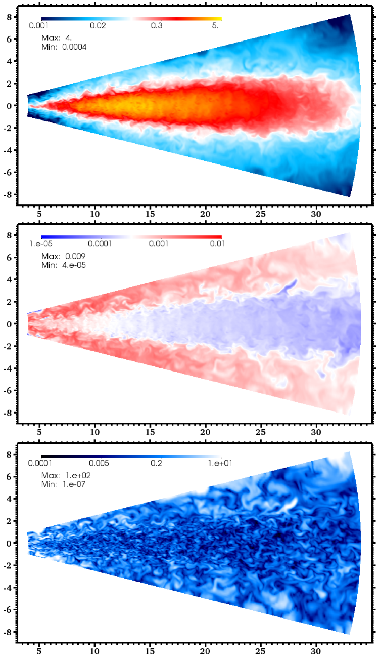
Figure 7.— Slices in the poloidal plane from model gbl-$m10+$ at $t=14\;P^{\rm orb}_{30}$ showing $\rho$ (upper), $T$ (middle), and $\beta^{-1}$ (lower).

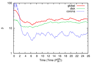
Figure 8.— Disk body, corona, and global volume averages of the plasma-$\beta$ for model gbl-$m10+$.

Fig. 7 shows a poloidal slice through the disk in model gbl-$m10+$ at $t=14~{}P^{\rm orb}_{30}$. During the turbulent steady state the disk is characterised by a dense, cold, sub-thermally magnetized core close to the mid-plane and a tenuous, hot, trans-to-super thermal magnetic field at $z\mathrel{\hbox to0.0pt{\lower 3.0pt\hbox{$\sim$}\hss}\raise 2.0pt\hbox{$>$}}2H$ (the corona). Turbulent motions are clearly evident in the plot of $\beta^{-1}$ in Fig. 7 with the dominant eddies appearing to have a larger size in the corona compared to the disk body. As noted by Fromang & Nelson (2006), such behaviour arises due to conservation of angular momentum in eddie motions - or wave action - as small scale eddies rise out of the dense disk mid-plane into the less dense coronal region. Our intended purpose for the explicit cooling function, $\Lambda$ (see § 2.1 for details) becomes more apparent from the temperature plot - we aim to take a step beyond the purely isothermal approximation and towards the observationally supported picture of a hot corona and cooler disk body. In Fig. 8 we show the volume-averaged plasma-$\beta$. In the disk body, we find $\overline{<\beta>}=17$ and for the corona $\overline{<\beta>}=6$. The coronal value is higher than values of close to one found in previous isothermal (Miller & Stone 2000; Flock et al. 2011) and quasi-isothermal simulations (Fromang & Nelson 2006; Beckwith et al. 2011), which may be attributable to the lack of any explicit cooling in the corona in our simulations. However, although the gas in the corona is heated by dissipation, it does not continually heat up through the simulation, and in fact remains quasi-steady through the latter half of the simulation. This contrasts with adiabatic shearing-box simulations with imposed periodic boundary conditions, in which the gas does heat up (e.g. Stone et al. 1996; Sano et al. 2004) and demonstrates that when coronal gas is allowed to freely expand, adiabatic cooling can, to some extent, balance heating via turbulent dissipation.

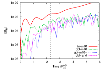
Figure 9.— Comparison of $|\delta B_{\rm R}(m=10,k_{\rm z}=5,k_{\rm R}=2.5)|$ from models lin-$m10$ (local linear MRI) and models gbl-$m10$, gbl-$m10+$, and gbl-rand (fully non-linear global simulations).

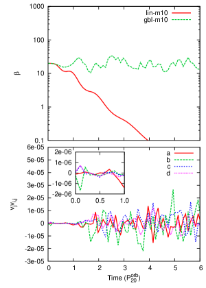
Figure 10.— Plasma-$\beta$ from models lin-$m10$ and gbl-$m10$ (upper), and time evolution of some sample non-linear terms in model gbl-$m10$ (lower).

4.2. Comparison with linear MRI growth estimates

In Fig. 9 we compare the evolution of $|\delta B_{\rm R}|$ for the $m=10$, $k_{\rm z}=5$, $k_{\rm R}=2.5$ mode (measured in Fourier space - see § 2.4) for model lin-$m10$ (which describes linear MRI growth - see Tables 2 and 1) and models gbl-$m10$ and gbl-$m10+$ (global simulations which allow fully non-linear evolution - see Table 3). Quantifying the initial growth by deriving approximate growth rates, $\omega_{\rm approx}$ for the curves shown in Fig. 9 , we find that the linear MRI estimate is matched best by model gbl-$m10+$, with gbl-$m10$ (and gbl-rand) producing higher growth rates. The higher amplitude perturbation for model gbl-$m10$ compared to gbl-$m10+$ originates from the larger amplitude initial velocity perturbation of $0.1~{}c_{\rm s}$ (compared to $0.001~{}c_{\rm s}$ for gbl-$m10+$ and gbl-rand - see Table 3). The agreement between the global simulations and linear growth estimate (model lin-$m10$) begins to falter after roughly $2~{}P^{\rm orb}_{20}$ and growth in $|\delta B_{\rm R}|$ for the global simulations levels off. From the linear MRI calculations shown in Fig. 2 one may anticipate that the growth in $|\delta B|$ is halted by the magnetic pressure evolving to equipartition with the gas pressure - which is illustrated by the vertical dashed line in Fig. 9 - and would mean that one cannot rely on model lin-$m10$ as a predictor for model gbl-$m10$. However, Fig. 10 shows that $\beta$ remains roughly constant in model gbl-$m10$ over the first few orbits. What then causes the local MRI estimates and the global simulations to diverge? In the lower panel of Fig. 10 we plot the evolution of the following non-linear terms derived from the momentum equations,

$$a=v_{\rm r}\frac{\partial v_{\rm r}}{\partial r},b=\frac{v_{\theta}}{r}\frac{\partial v_{\rm r}}{\partial\theta},$$

$$c=v_{\rm r}\frac{\partial v_{\theta}}{\partial r},d=\frac{v_{\theta}}{r}\frac{\partial v_{\theta}}{\partial\theta}.$$

Small spikes in these non-linear terms occur after $\sim 0.1$ orbit. However, after 1-2 orbits considerably larger fluctuations become apparent, particularly in $b$ which also appears to have the highest amplitude oscillations of the plotted terms thereafter. Considering that the linear MRI is seeded by velocity perturbations through the induction equation (Eqs (31) and (32)), the correlation in time between the non-linear velocity terms becoming active and the growth in $|\delta B_{\rm R}|$ departing from the linear MRI growth predictions is highly suggestive of non-linear motions causing saturation in the growth of a specific MRI mode. Furthermore, the small amplitude kicks from these non-linear terms after 0.1 orbits may explain the early divergence between the $\beta$ values predicted from model lin-$m10$ and those found from gbl-$m10$. In this sense the non-linear motions provide saturation to the initial phase of local $\delta{\bf B}$ growth. Whether the non-linear motions are attributable to secondary instabilities feeding off the linear MRI growth locally (e.g. Goodman & Xu 1994; Pessah et al. 2007; Pessah & Goodman 2009; Pessah 2010), or are due to the onset of turbulence (Latter et al. 2009) propagating radially outwards through the disk is unclear and would require an analysis of the non-linear growth of the non-axisymmetric MRI, which we do not pursue here.

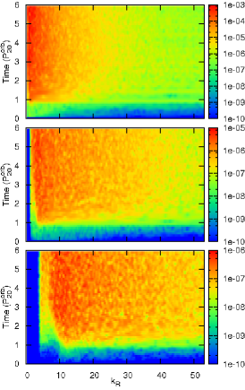
Figure 11.— Logarithmic false-colour image showing the time evolution of $|\delta B_{\rm R}({\bf k})|$ in model gbl-$m10+$. Values of $\delta B_{\rm R}$ in the disk body were Fourier transformed and results are shown at specific values of $m$ and $k_{\rm z}$, and the full range of $k_{\rm R}$. From top to bottom: $m=10$ and $k_{\rm z}=5$ (low wavenumber), $m=40$ and $k_{\rm z}=80$ (moderate wavenumber), and $m=120$ and $k_{\rm z}=150$ (high wavenumber).

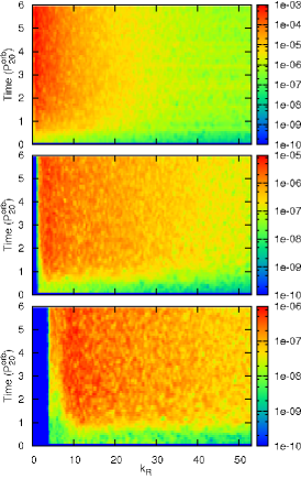
Figure 12.— Same as Fig. 11 except for model gbl-rand.

In summary, comparisons between linear growth calculations and global simulations highlights a number of potential saturation mechanisms. Such as, growth of magnetic field perturbations beyond the weak field limit, and/or growth of the radial wavenumber beyond the finite limit of the simulation resolution. However, for the simulations performed in this work, we find that saturation of growth in magnetic field perturbations correlates well with the onset of non-linear motions.

4.3. Trigger dependence

A major focus of magnetized accretion disk simulations is to study properties of the quasi-steady-state turbulence. A necessary test is whether the turbulent steady state depends on the MRI mode initially excited, and also whether prohibitive transient behaviour arises due to the choice of exciting a specific MRI mode. For this purpose we have computed model gbl-rand which uses the same initial disk as model gbl-$m10+$ with the difference that the disk is perturbed with random perturbations in the both the poloidal velocity (amplitude $\delta v_{0}=0.001~{}c_{\rm s}$) and gas pressure ($10\%$ amplitude) which excite a range of MRI modes. Simulation resolution and time-averaged measures of the turbulent state are listed in Tables 2 and 3, respectively.

The evolution of model gbl-rand is very similar to that of model gbl-$m10+$; the initial perturbations excite the MRI and lead to growth of $\delta B_{\rm R}$. Both models show similar growth in the $m=10$, $k_{\rm z}$, $k_{\rm R}=2.5$ mode (Fig. 9) which one would expect given that this mode is excited with the same amplitude perturbation. After $3~{}P^{\rm orb}_{20}$ ($\simeq 0.5~{}P^{\rm orb}_{30}$) values of $\delta B_{\rm R}$ become almost identical between the models irrespective of the differing initial perturbations. We illustrate this in Figs. 11 and 12 in which we show the evolution of $\delta B_{\rm R}$ in Fourier space for a range of $k_{\rm R}$ values. The different panels in the figures correspond to low, moderate, and high wavenumber values for $m$ and $k_{\rm z}$ (relative to the size of the disk and the Nyquist limit). As mentioned above, $\delta B_{\rm R}$ values are very similar between the two models at $t>3~{}P^{\rm orb}_{20}$. Furthermore, even though we excite a specific low wavenumber mode in model gbl-$m10$, a wide range of modes rapidly emerge. We attribute this behaviour to wave-wave coupling and the onset of a turbulent cascade.

Exciting larger wavenumbers should provide a larger initial MRI growth rate (see § 3), but how does this affect the evolution of magnetic field perturbations in the global simulations? In particular, does the wavenumber of the excited MRI mode affect the globally-averaged saturation stress? In model gbl-rand a white noise spectrum of perturbations has been excited. Therefore higher wavenumber modes can contribute to the initial growth phase in $<\alpha_{\rm P}>$. There is an indication of this from Fig. 12) where the growth of $|\delta B_{\rm R}|$ at a range of wavenumbers means that the Maxwell stress, and consequently $<\alpha_{\rm P}>$ will also grow across a range of wavenumbers. Fig. 4 shows that $<\alpha_{\rm P}>$ does grow faster for gbl-rand compared to gbl-$m10+$ (which have identical grid resolution), supporting the notion that the growth in the globally averaged stress due to an ensemble of unstable modes is higher than for a single wavenumber mode.

All three models start with a toroidal magnetic field with a net flux, and during the early evolution of the disk, the combination of magnetic buoyancy and accretion expels magnetic flux from the disk body such that by the time the turbulent steady state is reached the net toroidal magnetic flux of the disk, $\Psi_{\phi}$ is close to zero. Subsequently, $\Psi_{\phi}$ oscillates about the zero-point with a period of roughly $5$ orbits (upper panel of Fig. 13) consistent with previous global simulations and suggestive of a dynamo cycle (Fromang & Nelson 2006; O’Neill et al. 2011; Beckwith et al. 2011). All three models demonstrate this behaviour. However, minor differences in the toroidal magnetic flux, $\Psi_{\phi}$, are visible between models gbl-$m10+$ and gbl-rand (Fig. 13). The different models are slightly out of phase, which is not surprising given the differences in the transient evolution at early simulation times (Fig. 4). Interestingly, model gbl-rand does not overshoot when expelling the initial net toroidal flux and thus settles into dynamo oscillations at a slightly earlier time, which may explain why the transient phase in $<\alpha_{\rm P}>$ takes a longer time to fade in this model.

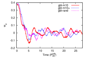
Figure 13.— Toroidal magnetic flux at $\phi=0$, $\Psi_{\phi}(\phi=0)$ as a function of time for models gbl-$m10$, gbl-$m10+$, and gbl-rand. See Eqs (20) for the definition of $\Psi_{\phi}$.

In conclusion, once the disk reaches a turbulent steady-state the disk retains no knowledge of the MRI mode initially excited. This is supported by the almost identical time-averaged properties of the disk noted in Table 3 for models perturbed by a single low wavenumber mode or an ensemble of modes.

4.4. Algorithm and resolution dependence

In this section we examine the ability of different numerical algorithms to recover the growth of magnetic field perturbations resulting from the non-axisymmetric MRI. Comparisons between numerical simulations and analytical estimates for the axisymmetric MRI have been presented by Hawley & Balbus (1991) and Flock et al. (2010). Considering that MHD turbulence in accretion disks produces a predominantly toroidal field it is important to examine how well numerical algorithms can recover the growth of $\delta{\bf B}$ as a result of the non-axisymmetric MRI. The setups used are listed in Table 2. The different combinations are intended to test different orders of reconstruction, parabolic limiters, and grid resolution. Reconstruction refers to the order of accuracy used to interpolate cell interface values (which are then used in the Riemann solver to calculate fluxes of conserved variables). Parabolic limiters are used to preserve monotonicity and prevent extrema from being introduced by the reconstruction step. We examine the original limiter for PPM proposed by Colella & Woodward (1984), the extremum preserving limiters presented by Colella & Sekora (2008), and limiters based on reconstruction via characteristic variables (e.g. Rider et al. 2007). The aforementioned slope limiters are respectively denoted “CW84”, “CS08”, and “Char” in Table 2. The last parameter we vary is the grid resolution, as this places a constraint on the maximum resolvable wavenumber, and for this purpose we compute models gbl-$m10$-hr, gbl-$m10$, gbl-$m10$-lr, gbl-$m10$-llr, and gbl-$m10$-lllr (which have decreasing resolution). Note that with the exception of models gbl-$m10+$ and gbl-rand, all models have the same cell aspect ratio and the same ratio of cells in the disk body to cells in the corona as gbl-$m10$.

As in § 4.2, we calculate approximate growth rates of the magnetic field perturbation, $|\delta B_{\rm R}({\bf k})|$ for the $m=10$, $k_{\rm z}=5$, $k_{\rm R}=2.5$ mode via a Fourier analysis of the initial simulation evolution. The results are shown in Table 2, which we summarise as follows:

• The best agreement with the linear MRI growth rate comes from model gbl-$m10+$, showing that azimuthal resolution is important for properly capturing MRI growth.

• Within errors the choice of limiter does not make a considerable difference to the resulting growth rate.

• Linear reconstruction produces a comparable growth rate to parabolic reconstruction.

• There is a consistent trend that growth rates increase with increasing resolution (see models gbl-$m10$-lllr, gbl-$m10$-llr, gbl-$m10$-lr, gbl-$m10$, and gbl-$m10$-hr). With 4 cells/$H$ in the $\phi$ direction the growth rates are converged (within errors) for roughly 23-35 cells/$H$ in the $z$ direction. This is a slightly lower threshold than the $\mathrel{\hbox to0.0pt{\lower 3.0pt\hbox{$\sim$}\hss}\raise 2.0pt\hbox{$>$}}40$ cells/$H$ (in the vertical direction) found to achieve convergence in the time-averaged turbulent stress in stratified shearing-box simulations (Davis et al. 2010). Comparison with model gbl-$m10+$ (which has 12.5 cells/$H$ in the $\phi$ direction) suggests that convergence in global disks may be achieved at lower resolutions when the cell aspect ratio is closer to unity.

5. Discussion

With a growing number of studies using stratified shearing boxes with high resolution and/or a large spatial extent (Shi et al. 2010; Davis et al. 2010; Guan & Gammie 2011; Simon et al. 2011, 2012) and higher resolution global models (Fromang & Nelson 2006; Sorathia et al. 2010, 2012; Flock et al. 2011, 2012; Beckwith et al. 2011; Hawley et al. 2011; Mignone et al. 2012), quantifying the steady state turbulence and making direct comparisons between simulations provides a check of both consistency and convergence.

One of the most popular measures of the steady state is $\overline{<\alpha_{\rm P}>}$. In this regard, models gbl-$m10+$ and gbl-rand produce values of $\sim 0.034$ which is higher than recently reported by Beckwith et al. (2011) and, as noted by these authors, higher than previous global models and a number of high resolution shearing-box simulations (see Hawley et al. 2011, and references there-in). We attribute the larger $\overline{<\alpha_{\rm P}>}$ in our models to a higher azimuthal resolution than used by (Beckwith et al. 2011), but also note the possible indication that higher $\overline{<\alpha_{\rm P}>}$’s may be more readily achievable in global simulations. Our average $\overline{<\alpha_{\rm M}>}\sim 0.41$ (for models gbl-$m10+$ and gbl-rand) is in good agreement with the $\sim 0.36-0.4$ achieved by the highest resolution shearing-box simulations to-date (Davis et al. 2010; Simon et al. 2011, 2012). Considering that our models have a lower number of cells/$H$ than the aforementioned shearing-box models, there may also be an indication that convergence may be achieved at lower grid resolutions than in localized models, potentially due to averaging over a larger volume, and capturing lower wavenumber eddies.

Comparing models gbl-$m10$ and gbl-$m10+$, strong evidence points to the grid cell aspect ratio and, in particular, the resolution in the $\phi$ direction as an important parameter in achieving a high $\overline{<\alpha_{\rm P}>}$ and $\overline{<\alpha_{\rm M}>}$ (see the discussion in Fromang & Nelson 2006, Flock et al. 2011, Hawley et al. 2011 and Sorathia et al. 2012). A possible explanation for this is that the dynamo cycle - which helps to sustain the turbulent state and involves the MRI as a driving agent - can operate more effectively at higher frequencies when the cell aspect ratio is closer to unity.

Related to $\overline{<\alpha_{\rm M}>}$ is the tilt angle, $\Theta_{\rm tilt}$, where $\sin 2\Theta_{\rm tilt}=<\alpha_{\rm M}>$ (Guan et al. 2009; Beckwith et al. 2011). It has been argued by Sorathia et al. (2012) that this parameter provides a better measure of convergence than $\overline{<\alpha_{\rm P}>}$, at least in the case of unstratified turbulence for which the question of convergence in the absence of explicit dissipation was raised by Fromang & Papaloizou (2007). We find $\Theta_{\rm tilt}\sim 9^{\circ}$ for model gbl-$m10$ which is consistent with previous findings for stratified global disks (Beckwith et al. 2011; Hawley et al. 2011; Flock et al. 2012). However, models gbl-$m10+$ and gbl-rand have $\Theta_{\rm tilt}\sim 12^{\circ}$ which is comparable to values of $\sim 11^{\circ}-13^{\circ}$ for shearing box simulations (both unstratified and stratified, e.g., Guan et al. 2009; Simon et al. 2012) and also for recent stratified global disks calculations performed with an orbital advection algorithm by Mignone et al. (2012). These results are encouraging as they show that global simulations are reaching sufficient grid resolution to reproduce shearing-box results.

The ratio of directional magnetic energy also provides insight into convergence and correspondence between simulations. We find, $\overline{<B_{\rm R}^{2}>/<B_{\phi}^{2}>}\sim 0.13$, $\overline{<B_{\rm z}^{2}>/<B_{\rm R}^{2}>}\sim 0.30$ and $\overline{<B_{\rm z}^{2}>/<B_{\phi}^{2}>}\sim 0.036$ for models gbl-$m10+$ and gbl-rand. These values are higher than obtained by Hawley et al. (2011) for their global disk simulations, and in some cases only slightly lower than values found from high resolution shearing-box simulations (Shi et al. 2010; Davis et al. 2010; Simon et al. 2011; Guan & Gammie 2011; Simon et al. 2012).

Interestingly, model gbl-$m10$ produces a sustained stress, albeit with a lower value than model gbl-$m10+$, but with only 4 cells/$H$ in the $\phi$-direction. Flock et al. (2011) found that at least 8 cells/$H$ were required to produce a sustained turbulent stress (see also Fromang & Nelson 2006). However, these authors used linear reconstruction, whereas we have used parabolic reconstruction which may permit a sustained stress at a slightly lower resolution.

Finally, we note that we do not see any prominent evidence of recurring transient phenomena due to linear growth revivals in the mean magnetic fields, as recently reported by Flock et al. (2012). This may be due to differences in the numerical setup between our models and those of Flock et al., or perhaps this phenomena occurs at later times that we have not reached with the simulation runtimes of our models.

6. Conclusions

We have performed global 3D MHD simulations of turbulent accretion disks which start from fully equilibrium MHD initial conditions. The local linear theory of the MRI is used as a predictor of the growth of magnetic field perturbations in the global simulations. Additional tests have also been performed to compare results obtained from global simulations using a number of different numerical algorithms and resolutions to the linear growth estimates. Our main findings are:

1. The growth of magnetic field perturbations in the global simulations shows good agreement with the linear MRI growth estimates during approximately the first orbit of the disk. Subsequently, the overwhelming influence of non-linear motions, which may be due either to the onset of turbulence or to secondary instabilities, saturates the local growth.

2. The saturated state is found to be independent of the initially excited MRI mode, showing that once the disk has expelled the initial net flux field and settled into quasi-periodic oscillations in the toroidal magnetic flux, the dynamo cycle regulates the global saturation stress level. Furthermore, time-averaged measures of quasi-steady turbulence are found to be in agreement with previous work. In particular, the time averaged stress, $\overline{<\alpha_{\rm P}>}\sim 0.034$.

3. We find $\overline{<B_{\rm R}^{2}>/<B_{\phi}^{2}>}\sim 0.13$ for global stratified simulations with 12.5 cells/$H$ in the $\phi$ direction, which is in good agreement with value found from high resolution, stratified, shearing-box simulations. Higher $\phi$ resolution in the simulation (at least $>4$ cells/$H$) is required to maintain stronger radial and vertical magnetic field, and consequently a larger $\overline{<\alpha_{\rm P}>}$.

4. From the numerical algorithms that we tested, the choice of reconstruction order or limiter does not significantly alter the resulting linear MRI growth rate. Convergence with resolution (for the linear MRI growth tests) is found for resolutions of roughly $23-35~{}$cells per scaleheight (in the vertical direction). However, above all, a higher azimuthal resolution contributes to a much better agreement with linear growth estimates, supporting the push for low cell aspect ratio (close to one) in global accretion disk simulations.

Acknowledgements

We thank the referee for a particularly useful report which helped to significantly improve the paper. This research was supported under the Australian Research Council’s Discovery Projects funding scheme (project number DP1096417). E. R. P thanks the ARC for funding through this project. This work was supported by the NCI Facility at the ANU and by the iVEC facility at the Pawsey Centre, Perth, WA.

Appendix A Equilibrium disk solutions

The initial conditions for our simulations are an equilibrium thin disk with a purely toriodal magnetic field. In the following we present some analytic solutions which are of use for numerical simulations of accretion disks and for disks in other environments, such as starburst galaxies (e.g. Cooper et al. 2008). These solutions incorporate more or less arbitrary radial profiles of density and temperature and a toroidal magnetic field. The latter involves either a constant ratio of gas-to-magnetic pressure, $\beta$, radially dependent $\beta$, constant $B_{\phi}$, and variants with net/zero toroidal magnetic flux.

In axisymmetric cylindrical coordinates ($R,\phi,z$), in steady-state, and with $v_{\rm R}=v_{\rm z}=B_{\rm R}=B_{\rm z}=0$, the induction equation is identically satisfied and we are left with the two momentum equations:

$$\frac{\partial P}{\partial R}+\rho\frac{\partial\Phi}{\partial R}-\frac{\rho v_{\phi}^{2}}{R}+\frac{1}{2R^{2}}\frac{\partial(R^{2}B_{\phi}^{2})}{\partial R} = 0,$$ (A1)

$$\frac{\partial P}{\partial z}+\rho\frac{\partial\Phi}{\partial z}+\frac{1}{2}\frac{\partial B_{\phi}^{2}}{\partial z} = 0,$$ (A2)

where the pressure, $P=\rho T$, with $T$ in scaled units.

We derive a compatibility condition for the above equations by subtracting $\partial/\partial R$ of Eq (A2) from $\partial/\partial z$ of Eq (A1), to obtain,

$$\frac{\partial}{\partial z}\left(\frac{v_{\phi}^{2}}{R}\right)=\frac{\partial T}{\partial z}\frac{1}{\rho}\frac{\partial\rho}{\partial R}-\frac{1}{2R^{2}\rho^{2}}\frac{\partial\rho}{\partial z}\frac{\partial(R^{2}B_{\phi}^{2})}{\partial R}+\frac{1}{\rho R}\frac{\partial B_{\phi}^{2}}{\partial z}-\frac{\partial T}{\partial R}\frac{1}{\rho}\frac{\partial\rho}{\partial z}+\frac{1}{2\rho^{2}}\frac{\partial\rho}{\partial R}\frac{\partial B_{\phi}^{2}}{\partial z}$$ (A3)

To solve for the disk equilibrium we take the approach of using Eq (A2) to derive an equation for $\rho(R,z)$, Eq (A3) to acquire $v^{2}_{\phi}(R,z)$, and Eq (A1) to obtain an expression for $v^{2}_{\phi}(R,0)$. The resulting equations require boundary conditions for the run of $\rho$ and $T$ at the disk midplane, which can be chosen arbitrarily. From here on we take the disk to be isothermal in height, $T=T(R)$, and firstly consider a disk with a constant, $\beta=2P/|B|^{2}\equiv 2P/B_{\phi}^{2}$. Eq (A2) then becomes,

$$\frac{1}{\rho}\frac{\partial\rho}{\partial z}=-\frac{\partial\Phi}{\partial z}\left(\frac{\beta}{1+\beta}\right)\frac{1}{T(R)}$$ (A4)

which integrates to give an expression for the density in terms of its midplane value,

$$\rho(R,z)=\rho(R,0)\exp\left(\frac{-\{\Phi(R,z)-\Phi(R,0)\}}{T(R)}\frac{\beta}{1+\beta}\right).$$ (A5)

Turning to the rotational velocity, the compatibility relation (Eq (A3)) reduces to,

$$\frac{\partial}{\partial z}\left(\frac{v_{\phi}^{2}}{R}\right)=-\left(\frac{1+\beta}{\beta}\right)\frac{1}{\rho}\frac{\partial\rho}{\partial z}\frac{\partial T}{\partial R}$$ (A6)

which upon integrating and using Eq (A4) leads to an expression for the azimuthal velocity in terms of its midplane value,

$$v_{\phi}^{2}(R,z)=v_{\phi}^{2}(R,0)+\{\Phi(R,z)-\Phi(R,0)\}\frac{R}{T}\frac{dT}{dR}.$$ (A7)

The model is completed with a midplane rotational velocity, which is determined by substituting Eq (A5) into Eq (A1). This gives

$$v_{\phi}^{2}(R,0)=R\frac{\partial\Phi(R,0)}{\partial R}+\frac{2T}{\beta}+\left(\frac{1+\beta}{\beta}\right)\left(\frac{RT}{\rho(R,0)}\frac{\partial\rho(R,0)}{\partial R}+R\frac{dT}{dR}\right).$$ (A8)

The first term is the square of the Keplerian velocity; the remaining terms are proportional to the square of the sound speed so that Eq (A8) represents a minor departure from a Keplerian disk.

A possible variation to the aforementioned disk would be to make $\beta$ radially dependent, i.e., $\beta=\beta(R)$. For example, one may choose to make $\beta(R)\propto\sin(kR)$, where $k$ is a radial wavenumber. In such a case Eq (A5) for $\rho(R,z)$ is unchanged. However, the expression for the rotational velocity becomes,

$$v_{\phi}^{2}(R,z)=v_{\phi}^{2}(R,0)+\{\Phi(R,z)-\Phi(R,0)\}\left(\frac{R}{T}\frac{dT}{dR}-\frac{1}{\beta(1+\beta)}\frac{\partial\beta}{\partial R}\right)$$ (A9)

where, following substitution in Eq (A1),

$$v_{\phi}^{2}(R,0)=R\frac{\partial\Phi(R,0)}{\partial R}+\frac{2T}{\beta}+\left(\frac{1+\beta}{\beta}\right)\left(\frac{RT}{\rho(R,0)}\frac{\partial\rho(R,0)}{\partial R}+R\frac{dT}{dR}\right)-\frac{RT}{\beta^{2}}\frac{\partial\beta}{\partial R}.$$ (A10)

Alternatively, one may desire a disk with a constant $B_{\phi}(R,z)=B_{\phi 0}$, in which case the magnetic pressure does not influence the density profile, leading to,

$$\rho(R,z)=\rho(R,0)\exp\left(\frac{-\{\Phi(R,z)-\Phi(R,0)\}}{T(R)}\right),$$ (A11)

and a corresponding velocity profile of,

$$v_{\phi}^{2}(R,z)=v_{\phi}^{2}(R,0)+\{\Phi(R,z)-\Phi(R,0)\}\frac{R}{T}\frac{dT}{dR}+v^{2}_{\rm A\phi}(R,z)-v^{2}_{\rm A\phi}(R,0),$$ (A12)

with,

$$v_{\phi}^{2}(R,0)=R\frac{\partial\Phi(R,0)}{\partial R}+v^{2}_{\rm A\phi}(R,0)+\left(\frac{RT}{\rho(R,0)}\frac{\partial\rho(R,0)}{\partial R}+R\frac{dT}{dR}\right),$$ (A13)

and where the Alfvén speed, $v_{\rm A\phi}(R,z)=B_{\phi 0}/\sqrt{\rho(R,z)}$.

As mentioned above, the radial profiles $\rho(R,0)$ and $T(R)$ required to complete the disk model may be chosen arbitrarily, subject to boundary constraints at the outer disk edge. As an example, we use simple functions inspired by the Shakura & Sunyaev (1973) disk model, modified by truncation of the density profile at a specified outer radius:

$$\rho(R,0) = \rho_{0}f(R,R_{0},R_{\rm out})\left(\frac{R}{R_{0}}\right)^{\epsilon},$$ (A14)

$$f(R,R_{0},R_{\rm out}) = \left(\sqrt{\frac{R_{\rm out}}{R}}+\sqrt{\frac{R_{\rm 0}}{R}}-\sqrt{\frac{R_{\rm out}R_{0}}{R^{2}}}-1\right),$$ (A15)

$$T(R) = T_{\rm 0}\left(\frac{R}{R_{0}}\right)^{\chi},$$ (A16)

where $\rho_{0}$ sets the density scale, $R_{0}$ and $R_{\rm out}$ are the radius of the inner and outer disk edge, respectively, and $\epsilon$ and $\chi$ set the slope of the density and temperature profiles, respectively. The tapering function, $f(R,R_{0},R_{\rm out})$ is used to truncate the disk at an inner and outer radius. In practice this function is normalized to give $\rho(R_{\rm max},0)=\rho_{0}$, where the radius of peak density, $R_{\rm max}$ is given by the positive root of the quadratic resulting from taking $\partial/\partial R$ of Eq (A14), namely,

$$\sqrt{R_{\rm max}}=\frac{a}{2}(\sqrt{R_{\rm out}}+\sqrt{R_{0}})+\frac{1}{2}\sqrt{a^{2}(\sqrt{R_{\rm out}}+\sqrt{R_{0}})^{2}-4(1-\epsilon^{-1})\sqrt{R_{0}R_{\rm out}}}$$ (A17)

where $a=1-(2\epsilon)^{-1}$. Once $R_{\rm max}$ is known it is straightforward to renormalize the density profile.

Finally, studies of turbulent dynamos in magnetized disks are often concerned with the net flux of the magnetic field (e.g. Brandenburg et al. 1995; Hawley et al. 1996; Fromang & Nelson 2006). For the initially purely toroidal field we have adopted in this paper the net flux of the disk is given by $\Psi_{\phi}=\int\int B_{\phi}dRdz$. Noting that in the above derivations we have used $\beta$ to relate $B_{\phi}^{2}$ to $P$, meaning $B_{\phi}=\pm\sqrt{2\rho T/\beta}$, i.e. we are free to choose the sign of $B_{\phi}$. Therefore, if a net flux field is required then one may set the sign of $B_{\phi}$ the same everywhere, whereas if one desires a zero-net flux field then, for example, one may choose to make $B_{\phi}$ anti-symmetric about the disk midplane.

Appendix B Fourier transform in cylindrical coordinates

We wish to evaluate the Fourier transform $F(\bf k)$ of a function $f({\bf r})=f(R,\phi,z)$ expressed in terms of cylindrical polar coordinates $(R,\phi,z)$. The definition of the Fourier transform is

$$F({\bf k})=\int\exp(i{\bf k\cdot r})f({\bf r})\>d^{3}x$$ (B1)

Cylindrical coordinates in real and Fourier space are expressed via the following equations:

$$\begin{array}[]{ c c l c c c l}x&=&R\cos\phi&&k_{\rm x}&=&k_{\rm R}\cos\psi\\ y&=&R\sin\phi&&k_{\rm y}&=&k_{\rm R}\sin\psi\\ z&=&z&&k_{\rm z}&=&k_{\rm z}\end{array}$$ (B2)

Hence,

$${\bf k\cdot r}=k_{\rm R}R\,\cos(\phi-\psi)+k_{z}z$$ (B3)

and

$$F({\bf k})=\int_{V}\exp[i(k_{\rm R}R\,\cos(\phi-\psi)+k_{z}z)]\,f(R,\phi,z)\>RdRd\phi dz$$ (B4)

where $V$ is the computational region, usually of the form:

$$R_{0}<R<R_{1}\qquad 0<\phi<2\pi\qquad-z_{0}<z<z_{0}$$ (B5)

We begin by constructing a Fourier series in the periodic azimuthal coordinate $\phi$:

$$f(R,\phi,z)=\sum_{m=-\infty}^{\infty}f_{m}(R,z)\,e^{-im\phi}$$ (B6)

where the coefficients $f_{m}(R,z)$ are given by:

$$f_{m}(R,z)=\frac{1}{2\pi}\int_{0}^{2\pi}f(R,\phi,z)e^{im\phi}\>d\phi$$ (B7)

We now make the change of angular variable $\chi=\phi-\psi$; the integration over $\chi$ is still over the interval $[0,2\pi]$ since all of the angular functions within the integrand have period $2\pi$. The Fourier transform can now be expressed as:

$$F({\bf k})=\sum_{m=-\infty}^{\infty}e^{im\psi}\int_{R_{0}}^{R_{1}}\left[\int_{-z_{0}}^{z_{0}}e^{ik_{z}z}f_{m}(R,z)\left[\int_{0}^{2\pi}e^{i(-m\chi+k_{\rm R}R\cos\chi)}\>d\chi\right]\>\>dz\right]RdR$$ (B8)

The angular integral can be expressed in terms of Bessel functions ($J_{m}(k_{\rm R}R)$):

$$\int_{0}^{2\pi}e^{i(-m\chi+k_{\rm R}R\cos\chi)}\>d\chi=2\pi\,i^{m}J_{m}(k_{\rm R}R)$$ (B9)

Hence,

$$F({\bf k})=2\pi\sum_{m=-\infty}^{\infty}i^{m}\,e^{im\psi}\>\int_{R_{0}}^{R_{1}}J_{m}(k_{\rm R}R)\>\left[\int_{-z_{0}}^{z_{0}}e^{ik_{z}z}f_{m}(R,z)\>dz\right]\>R\,dR$$ (B10)

Equation (B10) defines the following procedure:

1. Evaluate the angular coefficients:

   $$f_{m}(R,z)=\frac{1}{2\pi}\int_{0}^{2\pi}f(R,\phi,z)e^{im\phi}\>d\phi$$ (B11)

2. Then perform the integration in the $z$ direction:

   $$F_{m}(R,k_{z})=\int_{-z_{0}}^{z_{0}}e^{ik_{z}z}f_{m}(R,z)\>dz$$ (B12)

3. Finally, perform the (truncated) Hankel transform in the radial direction:

   $$\hat{F}_{m}(k_{\rm R},k_{z})=\int_{R_{0}}^{R_{1}}RJ_{m}(k_{\rm R}R)F_{m}(R,k_{z})\>R\,dR$$ (B13)

4. The Fourier transform of $f(R,\phi,z)$ is

   $$F(k_{\rm R},\psi,k_{z})=2\pi\sum_{m=-\infty}^{\infty}i^{m}\,e^{im\psi}\>\hat{F}_{m}(k_{\rm R},k_{z})$$ (B14)

Since the input data for $f(R,\phi,z)$ are on a grid, the azimuthal, vertical and radial wave numbers, $m,k_{\rm z}$ and $k_{\rm R}$, are limited by the Nyquist limit. Let the number of intervals in each coordinate direction be $(n_{\rm R},n_{\phi},n_{\rm z})$ and the grid increments be $(\Delta R,\Delta\phi,\Delta z)=[(R_{1}-R_{0})/n_{\rm R},2\pi/n_{\phi},2z_{0}/n_{\rm z}]$. The grid coordinates are $R_{u},\phi_{v},z_{w}$ where:

$$R_{u} =R_{0}+u\,\Delta R \quad u =0,~{}1,...,~{}n_{\rm R}-1$$ (B15)

$$\phi_{v} =v\,\Delta\phi \quad v =0,~{}1,...,~{}n_{\phi}-1$$

$$z_{w} =-z_{0}+w\,\Delta z \quad w =0,~{}1,...,~{}n_{\rm z}-1$$

The expressions for the azimuthal $f_{m}(R,z)$ and vertical $F_{m}(R,k_{z})$ parts of the Fourier transform can be approximated by discrete Fourier transforms as follows:

$$f_{m}(R_{u},z_{w}) \approx\frac{1}{n_{\phi}}\sum_{v=0}^{n_{\phi}-1}f(R_{u},\phi_{v},z_{w})\>\exp[2\pi imv/n_{\phi}] \quad m =0,~{}1,...,~{}n_{\phi}/2$$ (B16)

$$F_{m}(R_{u},k_{\rm z}) \approx\frac{2z_{0}}{n_{\rm z}}\exp[-ik_{\rm z}z_{0}]\>\sum_{w=0}^{n_{\rm z}-1}f_{m}(R_{u},z_{w})\>\exp[2\pi lw/n_{\rm z}] \quad l =0,~{}1,...,~{}n_{\rm z}/2 \quad k_{\rm z} =\frac{\pi}{z_{0}}\,l$$

The radial transform can be evaluated from

$$\hat{F}_{m}(k_{\rm R},k_{z})=k_{\rm R}^{-2}\int_{k_{\rm R}R_{0}}^{k_{\rm R}R_{1}}sJ_{m}(s)F_{m}(s/k_{\rm R},k_{z})\>ds$$ (B17)

More accurate versions of equations (B16) may be evaluated using the approach given in Press et al. (1986).

References

- Balbus & Hawley (1991) Balbus, S. A., & Hawley, J. F. 1991, ApJ, 376, 214
- Balbus & Hawley (1992) —. 1992, ApJ, 400, 610
- Balbus & Hawley (1998) —. 1998, Reviews of Modern Physics, 70, 1
- Balsara & Meyer (2010) Balsara, D. S., & Meyer, C. 2010, arXiv:1003.0018v1
- Beckwith et al. (2011) Beckwith, K., Armitage, P. J., & Simon, J. B. 2011, MNRAS, 416, 361
- Bodo et al. (2011) Bodo, G., Cattaneo, F., Ferrari, A., Mignone, A., & Rossi, P. 2011, ApJ, 739, 82
- Bodo et al. (2008) Bodo, G., Mignone, A., Cattaneo, F., Rossi, P., & Ferrari, A. 2008, A&A, 487, 1
- Brandenburg (2005) Brandenburg, A. 2005, AN, 326, 787
- Brandenburg et al. (1995) Brandenburg, A., Nordlund, A., Stein, R. F., & Torkelsson, U. 1995, ApJ, 446, 741
- Chandrasekhar (1960) Chandrasekhar, S. 1960, Proc. Nat. Acad. Sci., 46, 253
- Colella & Sekora (2008) Colella, P., & Sekora, M. D. 2008, J. Comput. Phys, 227, 7069
- Colella & Woodward (1984) Colella, P., & Woodward, P. R. 1984, J. Comput. Phys, 54, 174
- Cooper et al. (2008) Cooper, J. L., Bicknell, G. V., Sutherland, R. S., & Bland-Hawthorn, J. 2008, ApJ, 674, 157
- Davis et al. (2010) Davis, S. W., Stone, J. M., & Pessah, M. E. 2010, ApJ, 713, 52
- Flock et al. (2010) Flock, M., Dzyurkevich, N., Klahr, H., & Mignone, A. 2010, A&A, 516, A26
- Flock et al. (2012) Flock, M., Dzyurkevich, N., Klahr, H., Turner, N., & Henning, T. 2012, ApJ, 744, 144
- Flock et al. (2011) Flock, M., Dzyurkevich, N., Klahr, H., Turner, N. J., & Henning, T. 2011, ApJ, 735, 122
- Fromang & Nelson (2006) Fromang, S., & Nelson, R. P. 2006, A&A, 457, 343
- Fromang & Nelson (2009) —. 2009, A&A, 496, 597
- Fromang & Papaloizou (2007) Fromang, S., & Papaloizou, J. 2007, A&A, 476, 1113
- Gardiner & Stone (2008) Gardiner, T. A., & Stone, J. M. 2008, J. Comput. Phys, 227, 4123
- Goldreich & Lynden-Bell (1965) Goldreich, P., & Lynden-Bell, D. 1965, MNRAS, 130, 125
- Goodman & Xu (1994) Goodman, J., & Xu, G. 1994, ApJ, 432, 213
- Gressel (2010) Gressel, O. 2010, MNRAS, 405, 41
- Guan & Gammie (2011) Guan, X., & Gammie, C. F. 2011, ApJ, 728, 130
- Guan et al. (2009) Guan, X., Gammie, C. F., Simon, J. B., & Johnson, B. M. 2009, ApJ, 694, 1010
- Hawley (2000) Hawley, J. F. 2000, ApJ, 528, 462
- Hawley & Balbus (1991) Hawley, J. F., & Balbus, S. A. 1991, ApJ, 376, 223
- Hawley et al. (1995) Hawley, J. F., Gammie, C. F., & Balbus, S. A. 1995, ApJ, 440, 742
- Hawley et al. (1996) —. 1996, ApJ, 464, 690
- Hawley et al. (2011) Hawley, J. F., Guan, X., & Krolik, J. H. 2011, ApJ, 738, 84
- Hawley & Krolik (2002) Hawley, J. F., & Krolik, J. H. 2002, ApJ, 566, 164
- Latter et al. (2009) Latter, H. N., Lesaffre, P., & Balbus, S. A. 2009, MNRAS, 394, 715
- Lesur & Longaretti (2007) Lesur, G., & Longaretti, P.-Y. 2007, MNRAS, 378, 1471
- Lynden-Bell & Pringle (1974) Lynden-Bell, D., & Pringle, J. E. 1974, MNRAS, 168, 603
- Lyra et al. (2008) Lyra, W., Johansen, A., Klahr, H., & Piskunov, N. 2008, A&A, 479, 883
- McKinney et al. (2012) McKinney, J. C., Tchekhovskoy, A., & Blandford, R. D. 2012, MNRAS, 423, 3083
- Mignone et al. (2007) Mignone, A., Bodo, G., Massaglia, S., Matsakos, T., Tesileanu, O., Zanni, C., & Ferrari, A. 2007, ApJS, 170, 228
- Mignone et al. (2012) Mignone, A., Flock, M., Stute, M., Kolb, S. M., & Muscianisi, G. 2012, A&A, 545, 152
- Miller & Stone (2000) Miller, K. A., & Stone, J. M. 2000, ApJ, 534, 398
- Miyoshi & Kusano (2005) Miyoshi, T., & Kusano, K. 2005, J. Comput. Phys, 208, 315
- Noble et al. (2010) Noble, S. C., Krolik, J. H., & Hawley, J. F. 2010, ApJ, 711, 959
- O’Neill et al. (2011) O’Neill, S. M., Reynolds, C. S., Miller, M. C., & Sorathia, K. A. 2011, ApJ, 736, 107
- Paczyńsky & Wiita (1980) Paczyńsky, B., & Wiita, P. J. 1980, A&A, 88, 23
- Papaloizou & Terquem (1997) Papaloizou, J. C. B., & Terquem, C. 1997, MNRAS, 287, 771
- Pessah (2010) Pessah, M. E. 2010, ApJ, 716, 1012
- Pessah et al. (2007) Pessah, M. E., Chan, C.-k., & Psaltis, D. 2007, ApJ, 668, L51
- Pessah & Goodman (2009) Pessah, M. E., & Goodman, J. 2009, ApJ, 698, L72
- Press et al. (1986) Press, W. H., Flannery, B. P., & Teukolsky, S. A. 1986, Numerical recipes. The art of scientific computing, ed. Press, W. H., Flannery, B. P., & Teukolsky, S. A.
- Regev & Umurhan (2008) Regev, O., & Umurhan, O. M. 2008, A&A, 481, 21
- Rider et al. (2007) Rider, W. J., Greenough, J. A., & Kamm, J. R. 2007, J. Comput. Phys, 225, 1827
- Romanova et al. (2012) Romanova, M. M., Ustyugova, G. V., Koldoba, A. V., & Lovelace, R. V. E. 2012, MNRAS, 421, 63
- Sano et al. (2004) Sano, T., Inutsuka, S.-i., Turner, N. J., & Stone, J. M. 2004, ApJ, 605, 321
- Shafee et al. (2008) Shafee, R., McKinney, J. C., Narayan, R., Tchekhovskoy, A., Gammie, C. F., & McClintock, J. E. 2008, ApJ, 687, L25
- Shakura & Sunyaev (1973) Shakura, N. I., & Sunyaev, R. A. 1973, A&A, 24, 337
- Shi et al. (2010) Shi, J., Krolik, J. H., & Hirose, S. 2010, ApJ, 708, 1716
- Simon et al. (2012) Simon, J. B., Beckwith, K., & Armitage, P. J. 2012, MNRAS, 422, 2685
- Simon et al. (2009) Simon, J. B., Hawley, J. F., & Beckwith, K. 2009, ApJ, 690, 974
- Simon et al. (2011) —. 2011, ApJ, 730, 94
- Sorathia et al. (2010) Sorathia, K. A., Reynolds, C. S., & Armitage, P. J. 2010, ApJ, 712, 1241
- Sorathia et al. (2012) Sorathia, K. A., Reynolds, C. S., Stone, J. M., & Beckwith, K. 2012, ApJ, 749, 189
- Stone et al. (1996) Stone, J. M., Hawley, J. F., Gammie, C. F., & Balbus, S. A. 1996, ApJ, 463, 656
- Stone & Pringle (2001) Stone, J. M., & Pringle, J. E. 2001, MNRAS, 322, 461
- Terquem & Papaloizou (1996) Terquem, C., & Papaloizou, J. C. B. 1996, MNRAS, 279, 767
- Tout & Pringle (1992) Tout, C. A., & Pringle, J. E. 1992, MNRAS, 259, 604
- Velikhov (1959) Velikhov, E. P. 1959, J. Expl. Theoret. Phys., 36, 1398
- Vishniac (2009) Vishniac, E. T. 2009, ApJ, 696, 1021