Phonon-drag thermopower and hot-electron energy-loss rate in a Rashba spin-orbit coupled two-dimensional electron system

Abstract

We theoretically study phonon-drag contribution to the thermoelectric power and hot-electron energy-loss rate in a Rashba spin-orbit coupled two-dimensional electron system in the Bloch-Gruneisen (BG) regime. We assume that electrons interact with longitudinal acoustic phonons through deformation potential and with both longitudinal and transverse acoustic phonons through piezoelectric potential. Effect of the Rashba spin-orbit interaction on magnitude and temperature dependence of the phonon-drag thermoelectric power and hot-electron energy-loss rate are discussed. We numerically extract the exponent of temperature dependence of the phonon-drag thermopower and the energy-loss rate. We find the exponents are suppressed due to the presence of the Rashba spin-orbit coupling.

I Introduction

There has been a rapidly growing interest on spin-orbit coupled low-dimensional electron systems like two-dimensional electron systems (2DES) formed at semiconductor heterostructure interface, quantum wires, quantum dots zutic ; winkler ; cahay etc. The usefulness of the spin-orbit coupling in condensed matter system was realized after the proposal of spin field effect transistor by Datta and Das datta and thereafter, various interesting theoretical and experimental studies have been reported. One main goal is to control and manipulate the spin degree of freedom of charge carriers in nanostructures so that spin-based electronic devices wolf ; fabian ; david and quantum information processing technology can be developed. The coupling between electron’s spin and orbital angular momentum naturally arises when one makes non-relativistic approximation to the relativistic Dirac equation. There are various types of spin-orbit interaction (SOI) present in semiconductor heterostructures. Most commonly used SOI is the Rashba SOI (RSOI) rashba which is due to the structural inversion asymmetry in semiconductor heterostructures such as GaAs/AlGaAs. One can also increase the strength of the spin-orbit coupling with the help of an external gate voltage nitta ; mats . The RSOI modifies various properties cape ; grima ; mars ; chen ; zhang of a 2DES including the electron polaron effective mass, polaron binding energy, mobility, etc.

The electron-phonon interaction (EPI) plays an important role in determining transport properties of a 2DES. There are mainly two kind of mechanisms responsible for the EPI in semiconductor heterostructures, namely deformation potential (DP) and piezoelectric (PE) scattering potential. The deformation potential is the change in potential energy of an electron due to lattice deformation. In an inversion asymmetry host crystal, an electric polarization is induced due to lattice vibration and the potential corresponds to the electric polarization is known as piezoelectric potential. The electrons are scattered by the deformation and piezoelectric potentials and provides a non-zero contribution to the momentum relaxation time, in addition to other contributions coming from disorders, impurities etc. Numerous studies have been devoted to probe EPI by measuring low-temperature mobility price1 ; price2 ; price3 ; price4 ; ridley ; price5 ; dassarma of a 2DES in the Bloch-Gruneisen (BG) regime. The characteristic BG temperaturestormer is defined as $T_{BG}=2\hbar v_{s}k_{F}/k_{B}$ (where $v_{s}$ is the sound velocity and $k_{F}$ is the Fermi wave vector). When the temperature decreases below $T_{BG}$ phonon modes with higher energy are no longer able to be thermally excited and electrons are scattered by a small fraction of acoustic phonons with wave vector $q\leq 2k_{F}$ due to the phase space restriction. This leads to a sharp decrease in resistivity $\rho\sim T^{\nu}$, where the exponent $\nu$ varies for different systems and different electron-phonon scattering mechanisms. The BG temperature becomes $T_{BG}\sim 6.2$ K for a typical electron density $n_{e}\sim 10^{11}$ m^-2 and sound velocity $v_{s}\sim 5.12\times 10^{3}$ ms^-1.

Thermoelectric properties of various materials including 2DES have attracted much interest due to potential applications. With the application of an external temperature gradient ${\bm{\nabla}}T$ across a sample, an electric field ${\bf E}\propto{\bm{\nabla}}T$ is generated. The proportionality constant ($S$) between ${\bf E}$ and ${\bm{\nabla}}T$ is known as thermoelectric power or the Seebeck coefficient. There are mainly two contributions to the thermoelectric power $S$: diffusion thermopower $S_{d}$ and phonon-drag thermopower $S_{g}$. The applied temperature gradient gives rise to flow of electrons and phonons from hotter region to cooler region. The diffusion thermopower is solely due to flow of electrons and sensitive to the energy dependence of various scattering mechanisms such as ionized impurity scattering, surface roughness scattering etc. On the other hand, flow of phonons will try to drag the electrons from hotter region to cooler region due to EPI and giving rise to phonon-drag thermopower. Extensive theoretical and experimental investigations cantrell ; cantrell1 ; cantrell2 ; lyo ; karl ; ruf ; butcher ; kuba ; zianni ; fletcher1 ; miele ; butch ; fletcher2 ; tsao ; schm on phonon-drag thermopower of a 2DES without RSOI have been performed.

Another relevant mechanism for probing the EPI is the energy-loss rate $(P$) of hot electrons. When an electron system is subjected to uniform heating, electron temperature raises above that of the phonons. Hot electron relaxes to lower temperature via acoustic phonon emission. There are numerous experimental and theoretical studies dolgo ; basu ; sakaki ; hess ; kawamura ; Ma ; apple ; pipa ; stan ; kasa ; pros on hot-electron energy-loss rate of a 2DES without RSOI.

Unlike diffusion thermopower, both phonon-drag thermopower and hot-electron energy-loss rate depend only on EPI. Therefore, one can determine the electron-phonon coupling constant reliably by measuring $S_{g}$ and $P$.

Very recently, diffusive thermopower firoz and acoustic phonon-limited resistivity ghosh in a spin-orbit coupled 2DES have been studied. To the best of our knowledge, a detailed study of the effect of RSOI on phonon-drag thermopower and hot-electron energy-loss rate have not been studied yet. In this paper, we study phonon-drag contribution to the thermoelectric power and energy-loss rate of a Rashba spin-orbit coupled quasi-2DES in which two-dimensional electron wave vector ${\bf k}$ couples with three-dimensional phonon wave vector ${\bf Q}=({\bf q},q_{z})$. We consider both DP and PE scattering mechanisms responsible for the EPI. In the BG regime we find analytically that $S_{g}$ is proportional to $T^{4}$ and $T^{2}$ for DP and PE scattering, respectively. On the other hand, approximate analytical calculations show that the energy-loss rate is proportional to $T^{5}$ and $T^{3}$ for DP and PE scattering, respectively. However, our numerical results reveal that the exponents are $strongly$ dependent on the electron density and the Rashba spin-orbit coupling constant.

This paper is organized as follows. In section II we present all the analytical results of phonon-drag thermopower and energy-loss rate. Numerical results and discussions have been reported in section III. We summarize our work in section IV.

II Theoretical details

We consider a quasi-2DES formed at the interface of semiconductor heterostructures which has a finite thickness in the confining direction (say, $z$). Typically, the confining potential in the $z$-direction is a triangular potential. We assume that only the lowest sub-band due to transverse confinement is occupied by the electrons. Therefore, electrons are restricted to move in the $xy$ plane with wave vector ${\bf k}=(k_{x},k_{y})$. One can write the electron’s wave function as $\psi({\bf r})=\psi(x,y)\xi_{0}(z)$. The Fang-Howard wave function fang in the $z$-direction is given by $\xi_{0}(z)=\sqrt{b^{3}/2}ze^{-bz/2}$ with $b=(48\pi m^{\ast}e^{2}/\varepsilon_{0}\kappa\hbar^{2})^{1/3}\Big{(}n_{d}+11n_{e}/32\Big{)}^{1/3}$ as the variational parameter. Here, $m^{\ast}$ is the effective mass of an electron, $\kappa$ is the dielectric constant. Also, $\varepsilon_{0}$ is permittivity of free space, $n_{d}$ is the depletion charge density and $n_{e}$ is the density of electron.

The single electron Hamiltonian is given by

$$H=\frac{{\bf p}^{2}}{2m^{\ast}}\sigma_{0}+\frac{\alpha}{\hbar}\big{(}{\sigma}_{x}{p}_{y}-{\sigma}_{y}{p}_{x}\big{)},$$ (1)

where ${\bf p}=\hbar{\bf k}$ is the momentum operator for the electron, $\sigma_{0}$ is the ${2\times 2}$ identity matrix, $\alpha$ is the RSOI coupling constant and $\sigma_{x(y)}$ are the usual Pauli spin matrices. The energy eigenvalues and the normalized eigenstates corresponding to the above Hamiltonian are, respectively, given by

$$\epsilon_{k}^{\lambda}=\frac{\hbar^{2}k^{2}}{2m^{\ast}}+\lambda\alpha k$$ (2)

and

$$\psi_{\lambda}(x,y)=\frac{1}{\sqrt{2}}\begin{pmatrix}1\\ \lambda e^{-i\phi_{k}}\end{pmatrix}e^{i{\bf k}\cdot{\bf r}},$$ (3)

with $\lambda=\pm$ indicates two spin-split energy branches and $\tan\phi_{k}=k_{x}/k_{y}$. At a given Fermi energy $\epsilon_{F}$, the Fermi wave vectors for the two energy branches can be written as $k_{F}^{\lambda}=\sqrt{(k_{F}^{0})^{2}-k_{\alpha}^{2}}-\lambda k_{\alpha}$ with $k_{F}^{0}=\sqrt{2\pi n_{e}}$ and $k_{\alpha}=m^{\ast}\alpha/\hbar^{2}$. The velocity of an electron in a particular branch $\lambda$ is given by

$${v}_{k}^{\lambda}=\frac{1}{\hbar}\frac{\partial\epsilon_{k}^{\lambda}}{\partial k}=\frac{\hbar k}{m^{\ast}}+\lambda\frac{\alpha}{\hbar}.$$ (4)

II.1 Phonon-drag thermopower

We consider the interaction between electrons with two-dimensional wave vector ${\bf k}$ and acoustic phonon with three-dimensional wave vector ${\bf Q}$. To calculate phonon-drag thermopower we follow the explicit formula given in Referencescantrell1 ; cantrell2 for 2DES. With appropriate modifications the expression for phonon-drag thermopower in a Rashba spin-orbit coupled 2DES is given by

$$S_{g}^{\lambda} = \frac{e\tau_{p}}{2\sigma Ak_{B}T^{2}}\sum_{\lambda^{\prime}}\sum_{{\bf k},{\bf k^{\prime}},{\bf Q}}\hbar\omega_{Q}f(\epsilon_{k}^{\lambda})\Big{[}1-f(\epsilon_{k^{\prime}}^{\lambda^{\prime}})\Big{]}$$ (5)

$$\times W_{Q}^{\lambda\lambda^{\prime}}({\bf k},{\bf k^{\prime}})\Big{\{}\tau(\epsilon_{k}^{\lambda}){\bf v}_{k}^{\lambda}-\tau(\epsilon_{k^{\prime}}^{\lambda^{\prime}}){\bf v}_{k^{\prime}}^{\lambda^{\prime}}\Big{\}}\cdot{\bf v}_{p},$$

where $e$ is the electronic charge, $\tau_{p}$ is the phonon mean free time, $A$ is the area of the sample, $\sigma$ is the Drude conductivity, $k_{B}$ is the Boltzmann constant, $\omega_{Q}=v_{s}Q$, $\tau(\epsilon_{k})$ is the energy-dependent momentum relaxation time of an electron, $f(\epsilon)=[\mathrm{e}^{\beta(\epsilon-\mu)}+1]^{-1}$ is the Fermi-Dirac distribution function with $\beta=1/(k_{B}T)$, ${\bf v}_{k}^{\lambda}$ is the velocity of an electron in a particular branch $\lambda$, ${\bf v}_{p}$ is the phonon velocity defined as ${\bf v}_{p}=v_{s}{\bf Q}/Q$ and $W_{Q}^{\lambda\lambda^{\prime}}({\bf k},{\bf k^{\prime}})$ is the transition probability which is responsible for making transition of an electron from an initial state $|{\bf k},\lambda\rangle$ to a final state $|{\bf k^{\prime}},\lambda^{\prime}\rangle$ with the absorption of a phonon. The explicit form of the transition probability is given by the Fermi’s golden rule

$$W_{Q}^{\lambda\lambda^{\prime}}({\bf k},{\bf k^{\prime}})=\frac{2\pi}{\hbar}|C_{Q}^{\lambda\lambda^{\prime}}|^{2}N_{Q}\delta\Big{(}\epsilon_{k^{\prime}}^{\lambda^{\prime}}-\epsilon_{k}^{\lambda}-\hbar\omega_{Q}\Big{)}\delta_{{\bf k^{\prime}},{{\bf k}+{\bf q}}},$$ (6)

where $|C_{Q}^{\lambda\lambda^{\prime}}|^{2}$ is the matrix element responsible for the EPI and $N_{Q}=[\exp(\beta\hbar\omega_{Q})-1]^{-1}$ is the equilibrium phonon distribution function.

The matrix elements for DP and PE scatterings are respectively given by ghosh

$$|C_{Q}^{\lambda,\lambda^{\prime}}|_{DP}^{2}=\frac{D^{2}\hbar Q}{2\rho_{m}v_{sl}}\frac{1+\lambda\lambda^{\prime}\cos\gamma_{{\bf k}{\bf k^{\prime}}}}{2}\delta_{\lambda,\lambda^{\prime}}|I(q_{z})|^{2}$$ (7)

and

$$|C_{Q,{l(t)}}^{\lambda,\lambda^{\prime}}|_{PE}^{2} = \frac{(eh_{14})^{2}\hbar}{2\rho_{m}v_{s{l(t)}}}\frac{1+\lambda\lambda^{\prime}\cos\gamma_{{\bf k}{\bf k^{\prime}}}}{2\sqrt{q^{2}+q_{z}^{2}}}\delta_{\lambda,\lambda^{\prime}}$$

$$\times |I(q_{z})|^{2}A_{l{(t)}}({\bf q},q_{z}),$$

where $D$ is the DP coupling constant, $h_{14}$ is the relevant PE tensor component, $\rho_{m}$ is the mass density, $v_{sl(t)}$ is the longitudinal (transverse) component of sound velocity, $\gamma_{{\bf k}{\bf k^{\prime}}}$ is the angle between ${\bf k}$ and ${\bf k^{\prime}}$, $A_{l}({\bf q},q_{z})=9q_{z}^{2}q^{4}/[2(q_{z}^{2}+q^{2})^{3}]$ and $A_{t}({\bf q},q_{z})=(8q_{z}^{4}q^{2}+q^{6})/[4(q_{z}^{2}+q^{2})^{3}]$. The Kronecker delta symbol $\delta_{\lambda,\lambda^{\prime}}$ in the matrix elements implies that the EPI is spin-independent. Finally the form factor $|I(q_{z})|^{2}$ which is responsible for the finite thickness of the quasi-2DES and it has the form $|I(q_{z})|^{2}=|\int dz\xi_{0}^{2}(z)e^{iq_{z}z}|^{2}=b^{6}/(q_{z}^{2}+b^{2})^{3}$ for a triangular potential.

With the help of the Kronecker delta symbol $\delta_{{\bf k^{\prime}},{{\bf k}+{\bf q}}}$ in Eq. (6) the summation over ${\bf k}^{\prime}$ in Eq. (5) can be easily evaluated by replacing ${\bf k^{\prime}}$ with ${{\bf k}+{\bf q}}$. The argument of the delta function in Eq. (6) confirms the conservation of energy $\epsilon_{k^{\prime}}=\epsilon_{k}+\hbar\omega_{Q}$. At this point we assume that $\tau(\epsilon_{k})$ is approximately constant over an energy scale of the order of $\hbar\omega_{Q}$ so that we can write $\tau(\epsilon_{k}+\hbar\omega_{Q})\simeq\tau(\epsilon_{k})$. The summation over ${\bf k}$ in Eq. (5) can be converted into an integral over $\epsilon_{k}$ by the following transformation

$$\sum_{\bf k}\rightarrow\frac{A}{(2\pi)^{2}}\frac{m^{\ast}}{\hbar^{2}}\int d\epsilon_{k}\Big{(}1-\lambda\sqrt{\frac{\epsilon_{\alpha}}{\epsilon_{k}+\epsilon_{\alpha}}}\Big{)}\int d\theta,$$ (9)

where $\theta$ is the angle between ${\bf k}$ and ${\bf q}$. At very low temperature we can make an additional approximation as $f(\epsilon_{k})\{1-f(\epsilon_{k}+\hbar\omega_{Q})\}\simeq\hbar\omega_{Q}(N_{Q}+1)\delta(\epsilon_{k}-\epsilon_{F})$. Now we convert the summation over ${\bf Q}$ into an integration over $q$ and $q_{z}$ as $\sum_{\bf Q}\rightarrow(1/4\pi^{2})\int qdqdq_{z}$. In BG regime, phonon energy is very small compared to the Fermi energy and consequently we can make a further approximation as $q<<2k_{F}$. With all these assumptions described above taken into account one can obtain a final expression for the phonon-drag thermopower as (for intermediate steps see the Appendix A1)

$$S_{g}^{\lambda} = -\frac{e\tau_{p}v_{s}m^{\ast}\tau(\epsilon_{F})}{8\pi^{3}\hbar^{4}\sigma k_{B}T^{2}k_{F}^{\lambda}}\Big{(}1-\lambda\sqrt{\frac{\epsilon_{\alpha}}{\epsilon_{F}+\epsilon_{\alpha}}}\Big{)}$$ (10)

$$\times \int dqdq_{z}q^{2}\frac{|C_{Q}^{\lambda,\lambda^{\prime}}|^{2}}{Q}(\hbar\omega_{Q})^{2}N_{Q}(N_{Q}+1).$$

Here, we have assumed $\tau^{+}(\epsilon_{F})=\tau^{-}(\epsilon_{F})=\tau(\epsilon_{F})$ because the difference between $\tau^{+}$ and $\tau^{-}$ is very small.

The phonon energy is given by $\epsilon_{p}=\hbar\omega_{Q}=\hbar v_{s}\sqrt{q^{2}+q_{z}^{2}}$, so we can write $q=\epsilon_{p}\cos\phi/(\hbar v_{s})$ and $q_{z}=\epsilon_{p}\sin\phi/(\hbar v_{s})$ so that $dqdq_{z}\rightarrow\epsilon_{p}d\epsilon_{p}d\phi/(\hbar v_{s})^{2}$. We consider the quasi-2DES is very thin i.e. $q_{z}<<b$ so $|I(q_{z})|^{2}$ can be approximated as $|I(q_{z})|^{2}\simeq 1$. With these substitutions $S_{g}$ due to DP scattering becomes

$$S_{g}^{\lambda} = -\frac{e\tau_{p}m^{\ast}\tau(\epsilon_{F})}{8\pi^{3}\hbar^{4}\sigma k_{B}T^{2}k_{F}^{\lambda}}\Big{(}1-\lambda\sqrt{\frac{\epsilon_{\alpha}}{\epsilon_{F}+\epsilon_{\alpha}}}\Big{)}\frac{D^{2}\hbar}{2\rho_{m}}$$ (11)

$$\times \frac{1}{(\hbar v_{sl})^{4}}\int d\epsilon_{p}\epsilon_{p}^{5}N_{Q}(N_{Q}+1)\int d\phi\cos^{2}\phi.$$

Using the standard result $\int d\epsilon_{p}\epsilon_{p}^{n}N_{Q}(N_{Q}+1)=(n)!\zeta(n)(k_{B}T)^{n+1}$ with $\zeta(n)$ is the Riemann zeta function, we obtain

$$S_{g}^{\lambda}=-\frac{{m^{\ast}}^{2}\Lambda D^{2}k_{B}}{16\pi^{2}\rho_{m}n_{e}\hbar^{2}ek_{F}^{\lambda}}\Big{(}1-\lambda\sqrt{\frac{\epsilon_{\alpha}}{\epsilon_{F}+\epsilon_{\alpha}}}\Big{)}\frac{5!\zeta(5)(k_{B}T)^{4}}{(\hbar v_{sl})^{5}},$$ (12)

where $\Lambda=v_{sl}\tau_{p}$ is the phonon mean free path. The total phonon-drag thermopower due to DP scattering is given by

$$S_{g}^{DP}=-\frac{{m^{\ast}}^{2}\Lambda D^{2}k_{B}}{8\pi^{2}\hbar^{2}\rho_{m}n_{e}ek_{F}^{0}}\sqrt{\frac{\epsilon_{F}^{0}}{\epsilon_{F}^{0}-\epsilon_{\alpha}}}\frac{5!\zeta(5)(k_{B}T)^{4}}{(\hbar v_{sl})^{5}}.$$ (13)

The total phonon-drag thermopower $S_{g}$ for DP scattering is proportional to $T^{4}$.

Calculations similar to DP scattering will yield the total phonon-drag thermopower for longitudinal and transverse PE scatterings as

$$S_{g,l}^{PE}=-\frac{45{m^{\ast}}^{2}\Lambda(eh_{14})^{2}k_{B}}{2^{10}\pi^{2}\hbar^{2}\rho_{m}n_{e}ek_{F}^{0}}\sqrt{\frac{\epsilon_{F}^{0}}{\epsilon_{F}^{0}-\epsilon_{\alpha}}}\frac{3!\zeta(3)(k_{B}T)^{2}}{(\hbar v_{sl})^{3}}$$ (14)

and

$$S_{g,t}^{PE}=-\frac{59v_{st}{m^{\ast}}^{2}\Lambda(eh_{14})^{2}k_{B}}{2^{11}v_{sl}\pi^{2}\hbar^{2}\rho_{m}n_{e}ek_{F}^{0}}\sqrt{\frac{\epsilon_{F}^{0}}{\epsilon_{F}^{0}-\epsilon_{\alpha}}}\frac{3!\zeta(3)(k_{B}T)^{2}}{(\hbar v_{st})^{3}}.$$ (15)

Total phonon-drag thermopower due to PE scattering is given by $S_{g}^{PE}=S_{g,l}^{PE}+2S_{g,t}^{PE}$ and in this case $S_{g}^{PE}\sim T^{2}$.

II.2 Hot-electron Energy-loss rate

The average energy-loss rate per electron via acoustic phonon emission is given by

$$P=\Big{\langle}\frac{\partial\epsilon}{\partial t}\Big{\rangle}=\frac{1}{N_{e}}\sum_{\lambda,\bf Q}\hbar\omega_{Q}\Big{[}\frac{\partial N_{Q}}{\partial t}\Big{]}_{\lambda},$$ (16)

where $N_{e}$ is the total number of electrons. The rate of change of phonon occupation number for a given branch $\lambda$ is given by

$$\Big{[}\frac{\partial N_{Q}}{\partial t}\Big{]}_{\lambda} = \sum_{\bf k}W_{Q}^{\lambda\lambda}({\bf k},{\bf k}+{\bf q})\Big{\{}(N_{Q}+1)f(\epsilon_{k}^{\lambda}+\hbar\omega_{Q})$$

$$\times [1-f(\epsilon_{k}^{\lambda})]-N_{Q}f(\epsilon_{k}^{\lambda})[1-f(\epsilon_{k}^{\lambda}+\hbar\omega_{Q})]\Big{\}},$$

where the Fermi-Dirac distribution function $f(\epsilon)$ is described by the temperature of hot electrons $T_{e}$ and phonon distribution function is described by the lattice temperature $T_{l}$. Obviously $T_{e}$ is larger than $T_{l}$ so that electron can relax its energy via acoustic phonon emission and equilibrate to the lattice temperature.

Now we use the following identity

$$\frac{1-f(\epsilon_{\bf k}+\hbar\omega_{Q})}{1-f(\epsilon_{\bf k})}=\frac{f(\epsilon_{\bf k}+\hbar\omega_{Q})}{f(\epsilon_{\bf k})}e^{\beta_{e}\hbar\omega_{Q}},$$ (18)

with $\beta_{e}=1/(k_{B}T_{e})$. Using Eqs. (16) to (18) and taking all the assumptions made for calculating $S_{g}$ into account we finally obtain the following expression for energy-loss rate as (detail calculations are given in Appendix A2)

$$P = \frac{{m^{\ast}}^{2}}{4n_{e}\pi^{3}\hbar^{5}}\sum_{\lambda}\frac{1}{k_{F}^{\lambda}}\Big{(}1-\lambda\sqrt{\frac{\epsilon_{\alpha}}{\epsilon_{F}+\epsilon_{\alpha}}}\Big{)}^{2}\int dqdq_{z}$$ (19)

$$\times (\hbar\omega_{Q})^{2}|C_{Q}^{\lambda,\lambda^{\prime}}|^{2}\Big{\{}\frac{1}{e^{\beta_{e}\hbar\omega_{Q}}-1}-\frac{1}{e^{\beta_{l}\hbar\omega_{Q}}-1}\Big{\}},$$

with $\beta_{l}=1/(k_{B}T_{l})$. The integration over $q$ and $q_{z}$ in Eq. (19) can be easily evaluated by the same technique as described in the previous sub-section. The expressions for total energy relaxation rate for DP, longitudinal PE and transverse PE scattering are respectively given by

$$P^{DP}=\frac{{m^{\ast}}^{2}D^{2}k_{B}^{5}4!\zeta(5)}{2\pi^{2}n_{e}\rho_{m}\hbar^{7}v_{sl}^{4}k_{F}^{0}}\sqrt{\frac{\epsilon_{F}^{0}}{\epsilon_{F}^{0}-\epsilon_{\alpha}}}(T_{e}^{5}-T_{l}^{5}),$$ (20)

$$P_{l}^{PE}=\frac{9{m^{\ast}}^{2}(eh_{14})^{2}k_{B}^{3}2!\zeta(3)}{64\pi^{2}n_{e}\rho_{m}\hbar^{5}v_{sl}^{2}k_{F}^{0}}\sqrt{\frac{\epsilon_{F}^{0}}{\epsilon_{F}^{0}-\epsilon_{\alpha}}}(T_{e}^{3}-T_{l}^{3})$$ (21)

and

$$P_{t}^{PE}=\frac{13{m^{\ast}}^{2}(eh_{14})^{2}k_{B}^{3}2!\zeta(3)}{128\pi^{2}n_{e}\rho_{m}\hbar^{5}v_{st}^{2}k_{F}^{0}}\sqrt{\frac{\epsilon_{F}^{0}}{\epsilon_{F}^{0}-\epsilon_{\alpha}}}(T_{e}^{3}-T_{l}^{3}).$$ (22)

In the BG regime $P^{DP}$ is proportional to $T^{5}$ for DP scattering and $P^{PE}\sim T^{3}$ for PE scattering.

III Numerical Results

In the previous section we have presented approximated analytical results of the phonon-drag thermopower and energy-loss rate. In this section we discuss numerical results of phonon-drag thermopower and hot-electron energy-loss rate. To do this we solve Eqs. (5) and (16) numerically for both DP and PE scattering mechanisms in the low temperature regime. For the numerical calculations we consider material parameters of GaAs/AlGaAs heterostructures as $m^{\ast}=0.067m_{e}$ with free electron mass $m_{e}$, $\rho_{m}=5.31\times 10^{3}$ Kg m^-3, $v_{sl}=5.12\times 10^{3}$ ms^-1, $v_{st}=3.04\times 10^{3}$ ms^-1, $D=12$ eV, $h_{14}=1.2\times 10^{9}$ Vm^-1, $\kappa=12.91$, $n_{d}=10^{14}$ m^-2, $\alpha_{0}=10^{-11}$ eV m and $n_{0}=10^{15}$ m^-3.

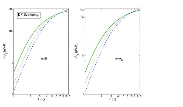
Figure 1: (Color online) Plots of the phonon-drag thermopower due to DP scattering versus temperature for different values of the density. Here, solid, dotted and dashed lines represent $n_{e}=3n_{0}$, $n_{e}=5n_{0}$ and $n_{e}=7n_{0}$, respectively.

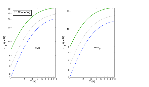
Figure 2: (Color online) Plots of the phonon-drag thermopower due to PE scattering versus temperature for different values of the density. Here, solid, dotted and dashed lines represent $n_{e}=3n_{0}$, $n_{e}=5n_{0}$ and $n_{e}=7n_{0}$, respectively.

We estimate the effective exponent from the log-log plot of the phonon-drag thermopower versus temperature due to DP scattering in Fig. 1 for both $\alpha=0$ and $\alpha=\alpha_{0}$ with different densities. At very low temperature ($T\sim$ 1-3 K), we obtain $\nu=3.449,3.942$ and $4.139$ for $n_{e}=3n_{0}$, $5n_{0}$ and $7n_{0}$, respectively, when $\alpha=0$. On the other hand, we obtain $\nu=2.846,3.294$ and $3.547$ for $n_{e}=3n_{0}$, $5n_{0}$ and $7n_{0}$, respectively, when $\alpha=\alpha_{0}$. The value of $\nu$ with $\alpha=\alpha_{0}$ gets lowered than that with $\alpha=0$. Figure 1 also depicts that the magnitude of $S_{g}$ with $\alpha=\alpha_{0}$ is less in comparison with $\alpha=0$.

In Fig. 2, the log-log plot of the phonon-drag thermopower versus temperature due to PE scattering is presented for different values of $\alpha$ and $n_{e}$. When $\alpha=0$, we obtain $\nu=1.688,1.961$ and $2.096$ for $n_{e}=3n_{0}$, $5n_{0}$ and $7n_{0}$, respectively. When $\alpha=\alpha_{0}$, we obtain $\nu=1.290,1.520$ and $1.658$ for $n_{e}=3n_{0}$, $5n_{0}$ and $7n_{0}$, respectively. Comparing Fig. 1 and Fig. 2, one can conclude that the magnitude of $S_{g}$ due to DP scattering is larger than that due to PE scattering.

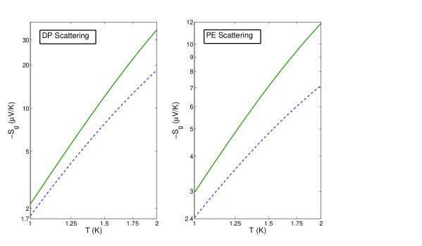
Figure 3: (Color online) Plots of the phonon-drag thermopower due to DP and PE scattering versus temperature for a fixed density $n_{e}=5n_{0}$. Here, solid and dashed lines represent $\alpha=0$ and $\alpha=\alpha_{0}$, respectively.

In Fig. 3 we plot $S_{g}$ due to DP and PE scattering versus $T$ for $\alpha=0$ and $\alpha=\alpha_{0}$ at a fixed density $n_{e}=5n_{0}$. Figure 3 clearly shows that slope of the line with $\alpha=\alpha_{0}$ is less than that with $\alpha=0$ case.

Figure 4: (Color online) Plots of the phonon-drag thermopower due to DP and PE scattering versus $\alpha$ for different values of the density at fixed temperature $T=2$K. Here, solid, dotted and dashed lines represent $n_{e}=3n_{0}$, $n_{e}=5n_{0}$ and $n_{e}=7n_{0}$, respectively.

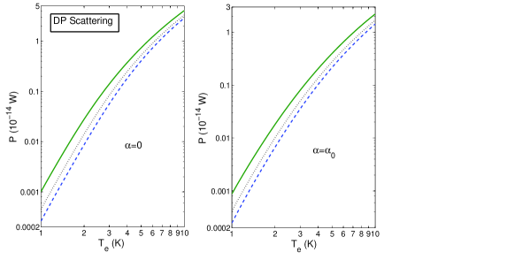
Figure 5: (Color online) Plots of the energy-loss rate due to DP scattering as a function of electron temperature $T_{e}$ for $\alpha=0$ and $\alpha=\alpha_{0}$ for different density. We set the lattice temperature $T_{l}=0$. Here, solid, dotted and dashed lines represent $n_{e}=3n_{0}$, $n_{e}=5n_{0}$ and $n_{e}=7n_{0}$, respectively.

Variation of $S_{g}$ due to DP and PE scattering as a function of the the Rashba coupling constant ($\alpha$) is shown in Fig. 4. The phonon-drag thermopower $S_{g}$ decreases very slowly with the increase of $\alpha$ in the case of both DP and PE scattering.

It is important to compare the order of magnitudes of diffusion and phonon-drag contributions to the total thermopower. The diffusion thermopower firoz is given by

$$S_{d}=-\frac{\pi^{2}k_{B}^{2}T}{3|e|\epsilon_{F}}\Big{(}p+1-\frac{\epsilon_{\alpha}}{\epsilon_{F}}\Big{)},$$ (23)

where the parameter $p$ depends on various scattering mechanisms. We calculate $S_{d}$ from Eq. (23) and $S_{g}$ from numerical evaluation of Eq. (5). With $\alpha=\alpha_{0}$ and $n=5n_{0}$ at $T=2$ K we obtain $S_{d}\sim-5.464$ $\mu$V$/$K, $S_{g}^{DP}\sim-18.526$ $\mu$V$/$K and $S_{g}^{PE}\sim-7.135$ $\mu$V$/$K. It is clear that at $T=2$ K the phonon-drag thermopower due to DP scattering dominates over both PE scattering induced phonon-drag thermopower and diffusion thermopower.

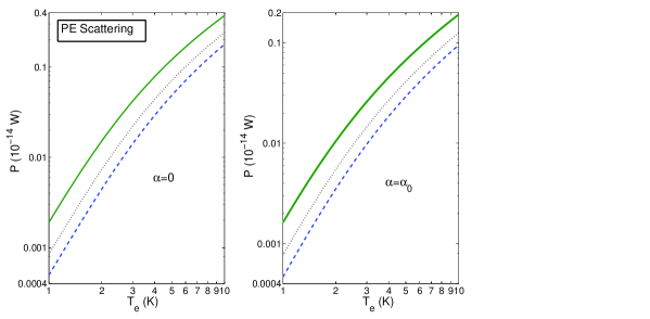
Figure 6: (Color online) Plots of the energy-loss rate due to PE scattering versus electron temperature $T_{e}$ for $\alpha=0$ and $\alpha=\alpha_{0}$ for different density. Here, lattice temperature is fixed to $T_{l}=0$. Solid, dotted and dashed lines represent $n_{e}=3n_{0}$, $n_{e}=5n_{0}$ and $n_{e}=7n_{0}$, respectively.

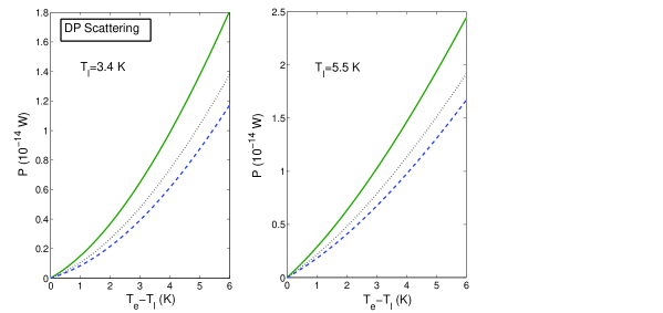
Figure 7: (Color online) Energy-loss rate due to DP scattering is plotted as a function of $T_{e}-T_{l}$ with $\alpha=\alpha_{0}$ for two lattice temperatures $T_{l}=3.4$ K and $T_{l}=5.5$ K. Here, solid, dotted and dashed lines represent $n_{e}=3n_{0}$, $n_{e}=5n_{0}$ and $n_{e}=7n_{0}$, respectively.

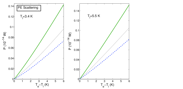
Figure 8: (Color online) Energy-loss rate due to PE scattering is plotted as a function of $T_{e}-T_{l}$ with $\alpha=\alpha_{0}$ for two lattice temperatures $T_{l}=3.4$ K and $T_{l}=5.5$ K. Here, solid, dotted and dashed lines represent $n_{e}=3n_{0}$, $n_{e}=5n_{0}$ and $n_{e}=7n_{0}$, respectively.

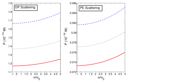
Figure 9: (Color online) Plots of the energy-loss rate due to DP and PE scattering versus $\alpha$ for different values of the lattice temperature $T_{l}$. We fix the electron temperature at $T_{e}=6$ K. Here, solid, dotted and dashed lines represent $T_{l}=3.4$ K, $T_{l}=4.2$ K and $T_{l}=5.5$ K, respectively.

Now we turn to present the numerical calculations for energy-loss rate of hot electrons in the BG regime. In Figs. 5 and 6 we have shown the dependence of $P$ with electron temperature $T_{e}$ for DP and PE scattering, respectively.

In general, energy-loss rate of hot-electrons is given by $P=\Gamma(T_{e}^{\delta}-T_{l}^{\delta})$ with $\Gamma$ as the proportionality constant. By taking the lattice temperature $T_{l}=0$ we determine the values of $\delta$ for $\alpha=0$ and $\alpha=\alpha_{0}$ from Figs. 5 and 6. For DP scattering with $\alpha=0$ the values of $\delta$ are $\delta=4.707,4.916$ and $4.998$ for $n_{e}=3n_{0},5n_{0}$ and $7n_{0}$, respectively. When $\alpha=\alpha_{0}$ we obtain $\delta=4.268,4.511$ and $4.661$ for $n_{e}=3n_{0},5n_{0}$ and $7n_{0}$, respectively. For PE scattering we find $\delta=2.945,3.078$ and $3.139$ for $n_{e}=3n_{0},5n_{0}$ and $7n_{0}$, respectively at $\alpha=0$. With $\alpha=\alpha_{0}$ the values of $\delta$ are obtained as $\delta=2.635,2.790$ and $2.880$ for $n_{e}=3n_{0},5n_{0}$ and $7n_{0}$, respectively.

Our numerical calculations reveal that the effective exponents of temperature dependence of phonon-drag thermopower and energy-loss rate strongly depend on the electron density and the Rashba spin-orbit coupling constant.

In Figs. 7 and 8 we plot $P$ due to DP and PE scattering as a function of $T_{e}-T_{l}$ with $\alpha=\alpha_{0}$ for different density. Different values of $T_{l}$ have been considered here. Magnitude of $P$ is higher at higher values of $T_{l}$ and it decreases with increase of the electron density. Comparing Figs. 7 and 8, we see that the energy-loss rate due to DP scattering is much higher than that due to PE case.

In Fig. 9, we present energy-loss rate due to DP and PE scattering versus $\alpha$ for different lattice temperatures. It shows the energy-loss rates increase monotonically with $\alpha$ in both the cases. This behavior is quite different from the behavior of the phonon-drag thermopower versus $\alpha$ shown in Fig. 4.

Density	DP		PE
$(n_{e})$	$\alpha=0$	$\alpha=\alpha_{0}$	$\alpha=0$	$\alpha=\alpha_{0}$
3$n_{0}$	3.449	2.846	1.688	1.290
5$n_{0}$	3.942	3.294	1.961	1.520
7$n_{0}$	4.139	3.547	2.096	1.658

Table 1: The effective exponent of the temperature dependence of $S_{g}$ in the BG regime for various values of $n_{e}$ and $\alpha$.

Density	DP		PE
$(n_{e})$	$\alpha=0$	$\alpha=\alpha_{0}$	$\alpha=0$	$\alpha=\alpha_{0}$
3$n_{0}$	4.707	4.268	2.945	2.635
5$n_{0}$	4.916	4.511	3.078	2.790
7$n_{0}$	4.998	4.661	3.139	2.880

Table 2: The effective exponent of the temperature dependence of $P$ in the BG regime for various values of $n_{e}$ and $\alpha$.

IV Summary

In this section we are summarizing the main results of the present work. In BG regime phonon-drag thermopower and hot-electron energy-loss rate have been calculated for quasi-2DES formed at the interface of GaAs/AlGaAs heterojunction. Both DP and PE scattering mechanism have been taken into account separately. It is shown that the effective exponent of the temperature dependence of the phonon-drag thermopower and energy-loss rate strongly depend on the electron density and the Rashba spin-orbit coupling constant. For DP and PE scattering in the BG regime, the values of the effective exponents of $T$ of thermoelectric power and hot-electron energy-loss rate for different values of $n_{e}$ and $\alpha$ are summarized in Table I and Table II.

It is shown that the order of magnitudes of phonon-drag thermopower due to DP and PE scattering are almost same and the phonon-drag thermopower dominates over the diffusion thermopower in the BG regime. The phonon-drag thermopower due to DP and PE scattering decreases very slowly with increase of $\alpha$.

The order of magnitude of the energy-loss rate due to DP scattering is much higher than that of the PE scattering. The energy-loss rate due to DP and PE scattering increases monotonically with $\alpha$.

Appendix A

In this appendix, we briefly sketch the derivation of the phonon-drag thermopower. Using Eqs. (5) and (9) we can write

$$S_{g}^{\lambda} = \frac{e\tau_{p}m^{\ast}}{8\pi^{2}\hbar^{2}\sigma k_{B}T^{2}}\sum_{\bf Q}\int d\epsilon_{k}\Big{(}1-\lambda\sqrt{\frac{\epsilon_{\alpha}}{\epsilon_{k}+\epsilon_{\alpha}}}\Big{)}$$ (24)

$$\times \int d\theta\hbar\omega_{Q}W_{Q}^{\lambda\lambda}({\bf k},{{\bf k}+{\bf q}})f(\epsilon_{k})\Big{\{}1-f(\epsilon_{k}+\hbar\omega_{Q})\Big{\}}$$

$$\times \tau(\epsilon_{k}^{\lambda})\Big{(}{\bf v}_{k}^{\lambda}-{\bf v}_{{\bf k}+{\bf q}}^{\lambda}\Big{)}\cdot{\bf v}_{p}.$$

Using the approximation $f(\epsilon_{k})\{1-f(\epsilon_{k}+\hbar\omega_{Q})\}\simeq\hbar\omega_{Q}(N_{Q}+1)\delta(\epsilon_{k}-\epsilon_{F})$, the integration over $\epsilon_{k}$ in Eq. (24) can be easily done and we obtain

$$S_{g}^{\lambda} = \frac{e\tau_{p}m^{\ast}\tau(\epsilon_{F})}{8\pi^{2}\hbar^{2}\sigma k_{B}T^{2}}\Big{(}1-\lambda\sqrt{\frac{\epsilon_{\alpha}}{\epsilon_{F}+\epsilon_{\alpha}}}\Big{)}\sum_{{\bf Q}}\int d\theta(\hbar\omega_{Q})^{2}$$

$$\times (N_{Q}+1)W_{Q}^{\lambda\lambda}({\bf k}_{F},{{\bf k}_{F}+{\bf q}})\Big{(}{\bf v}_{{\bf k}_{F}}^{\lambda}-{\bf v}_{{{\bf k}_{F}}+{\bf q}}^{\lambda}\Big{)}\cdot{\bf v}_{p}.$$

Using Eq. (4) and taking $q<<k_{F}$ we can write the difference between two velocities as

$${\bf v}_{{\bf k}_{F}}^{\lambda}-{\bf v}_{{{\bf k}_{F}}+{\bf q}}^{\lambda}\simeq-\frac{\hbar{\bf q}}{m^{\ast}}-\lambda\frac{\alpha}{\hbar}\Big{(}\frac{{\bf q}}{k_{F}}-\frac{{{\bf k}_{F}}({\bf k}_{F}\cdot{\bf q})}{k_{F}^{3}}\Big{)}.$$ (26)

Similarly, the difference between two energies can be approximated as

$$\epsilon_{{\bf k}_{F}+{\bf q}}^{\lambda}-\epsilon_{{\bf k}_{F}}^{\lambda} \simeq \Big{(}\frac{\hbar^{2}k_{F}}{m^{\ast}}+\lambda\alpha\Big{)}q\cos\theta$$ (27)

$$+ \Big{(}\frac{\hbar^{2}}{2m^{\ast}}+\lambda\frac{\alpha}{2k_{F}}\Big{)}q^{2},$$

where $\theta$ is the angle between ${\bf k}_{F}$ and ${\bf q}$. Converting the summation over ${\bf Q}$ into an integration over $q$, $q_{z}$ and doing the $\theta$ integration we can simplify Eq. (A) as

$$S_{g}^{\lambda} = -\frac{e\tau_{p}v_{s}{m^{\ast}}^{2}\tau(\epsilon_{F})}{8\pi^{3}\hbar^{5}\sigma k_{B}T^{2}{k_{F}^{\lambda}}^{2}}\Big{(}1-\lambda\sqrt{\frac{\epsilon_{\alpha}}{\epsilon_{F}+\epsilon_{\alpha}}}\Big{)}^{2}\int dqdq_{z}q^{2}$$ (28)

$$\times (\hbar\omega_{Q})^{2}N_{Q}(N_{Q}+1)\frac{|C_{Q}|^{2}}{QG(k_{F}^{\lambda},Q)}\Big{[}\frac{\hbar k_{F}^{\lambda}}{m^{\ast}}+\lambda\frac{\alpha}{\hbar}$$

$$- \lambda\frac{\alpha}{\hbar}\Big{\{}\frac{m^{\ast}v_{s}}{\hbar k_{F}^{\lambda}}\frac{Q}{q}\Big{(}1-\lambda\sqrt{\frac{\epsilon_{\alpha}}{\epsilon_{F}+\epsilon_{\alpha}}}\Big{)}-\frac{q}{2k_{F}^{\lambda}}\Big{\}}^{2}\Big{]},$$

with

$$G(k_{F}^{\lambda},Q) = \Big{\{}1-\frac{q^{2}}{4{k_{F}^{\lambda}}^{2}}+\frac{m^{\ast}v_{s}}{\hbar k_{F}^{\lambda}}\frac{Q}{k_{F}^{\lambda}}\Big{(}1-\lambda\sqrt{\frac{\epsilon_{\alpha}}{\epsilon_{F}+\epsilon_{\alpha}}}\Big{)}$$ (29)

$$- \Big{(}\frac{m^{\ast}v_{s}}{\hbar k_{F}^{\lambda}}\Big{)}^{2}\frac{Q^{2}}{q^{2}}\Big{(}1-\lambda\sqrt{\frac{\epsilon_{\alpha}}{\epsilon_{F}+\epsilon_{\alpha}}}\Big{)}^{2}\Big{\}}^{\frac{1}{2}}.$$

With the assumptions $q<<2k_{F}$ and $m^{\ast}v_{s}<<\hbar k_{F}$ we have $G(k_{F},Q)\simeq 1$. Eq. (10) can be derived easily from Eq. (28) with all the above mentioned approximations taken into account.

Appendix B

In this appendix, we briefly we outline the derivation of the energy-loss rate of hot electrons. Using Eq. (9) and after doing the integration over $\theta$, Eq. (II.2) can be re-written as

$$\Big{[}\frac{\partial N_{Q}}{\partial t}\Big{]}_{\lambda} = \frac{{m^{\ast}}^{2}A}{\pi\hbar^{5}q}\int d\epsilon_{\bf k}\Big{(}1-\sqrt{\frac{\epsilon_{\alpha}}{\epsilon_{\bf k}+\epsilon_{\alpha}}}\Big{)}^{2}$$ (30)

$$\times \frac{|C_{Q}|^{2}}{k^{\lambda}G(k^{\lambda},Q)}N_{Q}(T_{l})\Big{[}e^{(\beta_{l}-\beta_{e})\hbar\omega_{Q}}-1\Big{]}$$

$$\times f(\epsilon_{\bf k})\{1-f(\epsilon_{\bf k}+\hbar\omega_{Q})\}.$$

At low temperature we use the same approximation made in Appendix A. After doing the integration over $\epsilon_{\bf k}$ in Eq. (30) finally Eq. (16) becomes

$$P = \frac{{m^{\ast}}^{2}}{4\pi^{3}n_{e}\hbar^{5}}\sum_{\lambda}\Big{(}1-\lambda\sqrt{\frac{\epsilon_{\alpha}}{\epsilon_{F}+\epsilon_{\alpha}}}\Big{)}^{2}\int dqdq_{z}(\hbar\omega_{Q})^{2}$$

$$\times \frac{|C_{Q}|^{2}}{k_{F}^{\lambda}G(k_{F}^{\lambda},Q)}N_{Q}(T_{l})\{N_{Q}(T_{e})+1\}\Big{[}e^{(\beta_{l}-\beta_{e})\hbar\omega_{Q}}-1\Big{]}.$$

By taking the approximation $G(k_{F},Q)\simeq 1$ into account at low temperature and after evaluating the integrations over $q$ and $q_{z}$ in Eq. (B) it is not difficult to get Eqs. (20)-(22).

References

(1)
F. Fabian, A. Matos-Abiague, C. Ertler, P. Stano, and
I. Zutic, Acta Physica Slovaca 57, 565 (2007)
(arXiv: 0711.1461v1).
(2)
R. Winkler, Spin-Orbit Coupling Effects in
Two-Dimensional Electron and Hole Systems
(Springer Verlag-2003).
(3)
S. Bandyopadhyay and M. Cahay, Introduction to
Spintronics (CRC press-2008).
(4)
S. Datta and B. Das,
Appl. Phys. Lett. 56, 665 (1990).
(5)
S. A. Wolf, D. D. Awschalom, R. A. Burhman, J. M. Daughton, S. von Molnar,
M. L. Roukes, A. Y. Chtchelkanova, and D. M. Treger,
Science 294, 1488 (2001).
(6)
D. D. Awschalom and M. E. Flatte,
Nature Physics 3, 153 (2007).
(7)
I. Zutic, J. Fabian, and S. Das Sarma,
Rev. Mod. Phys. 76, 323 (2004).
(8)
E. I. Rashba, Fiz. Tverd. Tela (Leningrad) 2, 1224 (1960)
[Sov. Phys. Solid State 2, 1109 (1960)];
Y. A. Bychkov and E. I. Rashba, J. Phys. C 17, 6039 (1984).
(9)
J. Nitta, T. Akazaki, H. Takayanagi, and T. Enoki,
Phys. Rev. Lett. 78, 1335 (1997).
(10)
T. Matsuyama, R. Kursten, C. Meibner, and U. Merkt
Phys. Rev. B 61, 15588 (2000).
(11)
E. Cappelluti, C. Grimaldi, and F. Marsiglio,
Phys. Rev. B 76, 085334 (2007).
(12)
E. Cappelluti, C. Grimaldi, and F. Marsiglio,
Phys. Rev. Lett. 98, 167002 (2007).
(13)
C. Grimaldi, E. Cappelluti, and F. Marsiglio,
Phys. Rev. Lett. 97, 066601 (2006).
(14)
L. Chen, Z. Ma, J. C. Cao, T.Y. Zhang, and C. Zhang,
Appl. Phys. Lett. 91, 102115 (2007).
(15)
Z. Li, Z. S. Ma, A. R. Wright, and C. Zhang,
Appl. Phys. Lett. 90, 112103 (2007).
(16)
P. J. Price,
Ann. Physics (NY) 133, 217 (1981).
(17)
P. J. Price,
J. Vac. Sci. Technol. 19, 599 (1981).
(18)
P. J. Price,
Surf. Sci. 113, 199 (1982).
(19)
P. J. Price,
Surf. Sci. 143, 145 (1984).
(20)
B. K. Ridley,
J. Phys. C: Solid State Phys. 15, 5899 (1982).
(21)
P. J. Price,
Solid State Commun. 51, 607 (1984).
(22)
T. Kawamura and S. Das Sarma,
Phys. Rev. B 45, 3612 (1992).
(23)
H. L. Stormer, L. N. Pfeiffer, K. W. Baldwin, and K. W. West,
Phys. Rev. B 41, 1278 (1990).
(24)
D. G. Cantrell and P. N. Butcher,
J. Phys. C 19, L429 (1986).
(25)
D. G. Cantrell and P. N. Butcher,
J. Phys. C 20, 1985 (1987).
(26)
D. G. Cantrell and P. N. Butcher,
J. Phys. C 20, 1993 (1987).
(27)
S. K. Lyo,
Phys. Rev. B 38, 6345 (1988).
(28)
H. Karl, W. Dietsche, A. Fischer, and K. Ploog,
Phys. Rev. Lett. 61, 2360 (1988).
(29)
C. Ruf, H. Obloh, B. Junge, E. Gmelin, K. Ploog,
and G. Wiemann,
Phys. Rev. B 37, 6377 (1988).
(30)
M. J. Smith and P. N. Butcher,
J. Phys.: Condens. Matter 1, 1261 (1989).
(31)
S. S. Kubakaddi, P. N. Butcher, and B. G. Mulimani,
Phys. Rev. B 40, 1377 (1989).
(32)
X. Zianni, P. N. Butcher, and M. J. Kearney,
Phys. Rev. B 49, 7520 (1994).
(33)
R. Fletcher, V. M. Pudalov, Y. Feng,
M. Tsaousidou, and P. N. Butcher,
Phys. Rev. B 56, 12422 (1997).
(34)
A. Miele, R. Fletcher, E. Zaremba, Y. Feng,
C. T. Foxon, and J. J. Harris,
Phys. Rev. B 58, 13181 (1998).
(35)
P. N. Butcher and M. Tsaousidou,
Phys. Rev. Lett. 80, 1718 (1998).
(36)
R. Fletcher, Semicond. Sci. Technol. 14, R1 (1999).
(37)
M. Tsaousidou, The Oxford Handbook of Nanoscience and Technology
(Oxford University Press ), 2, 477 (2010).
(38)
M. Schmidt, G. Schneider, Ch. Heyn, A. Stemmann, and W. Hansen,
Phys. Rev. B 85, 075408 (2012).
(39)
V. T. Dolgopolov, A. A. Shashkin, S. I. Dorozhkin, and
E. A. Vyrodov,
Sov. Phys. JETP 62(6), 1219 (1985).
(40)
P. K. Basu and S. Kundu,
Appl. Phys. Lett. 47, 264 (1985).
(41)
K. Hirakawa and H. Sakaki,
Appl. Phys. Lett. 49, 889 (1986).
(42)
S. J. Manion, M. Artaki, M. A. Emanuel,
J. J. Coleman, and K. Hess,
Phys. Rev. B 35, 9203 (1987).
(43)
T. Kawamura, S. Das Sarma,
R. Jalabert, and J. K. Jain,
Phys. Rev. B 42, 5407 (1990).
(44)
Y. Ma, R. Fletcher, E. Zaremba,
M. D’Iorio, C. T. Foxon, and J. J. Harris,
Phys. Rev. B 43, 9033 (1991).
(45)
N. J. Appleyard, J. T. Nicholls, M. Y. Simmons,
W. R. Tribe, and M. Pepper,
Phys. Rev. Lett. 81, 3491 (1998).
(46)
V. I. Pipa, F. T. Vasko, and V. V. Mitin,
J. Appl. Phys. 85, 2754 (1999).
(47)
N. M. Stanton, A. J. Kent, S. A. Cavill,
A. V. Akimov, K. J. Lee, J. J. Harris, T. Wang,
and S. Sakai,
Phys. Stat. Sol(b) 228, 607 (2001).
(48)
S. S. Kubakaddi, K. Suresha, and B. G. Mulimani,
Physica E 18, 475 (2003).
(49)
Y. Y. Proskuryakov, J. T. Nicholls, D. I. Hadji-Ristic,
A. Kristensen, and C. B. Sorensen,
Phys. Rev. B 75, 045308 (2007).
(50)
SK F. Islam and T. K. Ghosh,
J. Phys.: Condens. Matter 24, 345301 (2012).
(51)
T. Biswas and T. K. Ghosh,
J. Phys.: Condens. Matter 25, 035301 (2013).
(52)
F. F. Fang and W. E. Howard,
Phys. Rev. Lett. 16, 797 (1966).