A Tractable Framework for Exact Probability of Node Isolation and Minimum Node Degree Distribution in Finite Multi-hop Networks

Zubair Khalid, Member, IEEE, Salman Durrani, Senior Member, IEEE  and Jing Guo, Student Member, IEEE The authors are with the Research School of Engineering, College of Engineering and Computer Science, The Australian National University, Canberra, ACT 0200, Australia. Emails: {zubair.khalid, salman.durrani, jing.guo}@anu.edu.au
Abstract

This paper presents a tractable analytical framework for the exact calculation of the probability of node isolation and the minimum node degree distribution when N𝑁N sensor nodes are independently and uniformly distributed inside a finite square region. The proposed framework can accurately account for the boundary effects by partitioning the square into subregions, based on the transmission range and the node location. We show that for each subregion, the probability that a random node falls inside a disk centered at an arbitrary node located in that subregion can be expressed analytically in closed-form. Using the results for the different subregions, we obtain the exact probability of node isolation and minimum node degree distribution that serves as an upper bound for the probability of k𝑘k-connectivity. Our theoretical framework is validated by comparison with the simulation results and shows that the minimum node degree distribution serves as a tight upper bound for probability of k𝑘k-connectivity. The proposed framework provides a very useful tool to accurately account for the boundary effects in the design of finite wireless networks.

Index Terms:
Wireless multi-hop networks, sensor networks, probability of node isolation, node degree distribution, probability of connectivity, k𝑘k-connectivity.

I Introduction

Wireless multi-hop networks, also refereed to as wireless sensor networks and wireless ad hoc networks, consist of a group of sensor nodes deployed over a finite region [1, 2, 3, 4, 5]. The nodes operate in a decentralized manner without the need of any fixed infrastructure, i.e., the nodes communicate with each other via a single-hop wireless path (if they are in range) or via a multi-hop wireless path. In most of the applications, such wireless networks are formed by distributing a finite (small) number of nodes in a finite area, which is typically assumed to be a square region [6, 7, 8, 9].

Connectivity is a basic requirement for the planning and effective operation of wireless multi-hop networks [10, 11]. The k𝑘k-connectivity is a most general notion of connectivity and an important characteristic of wireless multi-hop networks [12, 9, 13]. The network being k𝑘k-connected ensures that there exists at least k𝑘k independent multi-hop paths between any two nodes. In other words, k𝑘k-connected network would still be 111-connected if (k1)𝑘1(k-1) nodes forming the network fail. The probability of node isolation, defined as the probability that a randomly selected node has no connections to any other nodes, plays a key role in determining the overall network connectivity (1-connectivity) [12, 14]. The minimum node degree distribution, which is the probability that each node in the network has at least k𝑘k neighbours, is crucial in determining the k𝑘k-connectivity of the network [12].

For large-scale wireless sensor networks, assuming Poisson distributed nodes in an infinite area, the connectivity properties such as probability of isolation, average node degree, k𝑘k-connectivity have been well studied [15, 16, 12, 17, 18, 19, 20, 21]. When the node locations follow an infinite homogeneous Poisson point process and assuming all nodes have the same transmission range, it has been shown that the network becomes k𝑘k-connected with high probability (close to 111) at the same time the minimum node degree of the network approaches k𝑘k [15]. This fact was used to approximate the probability of k𝑘k-connectivity by the minimum node degree distribution in [12]. It was also used to determine the asymptotic value of the minimum transmission range for k𝑘k-connectivity for a uniform distribution of nodes in a unit square and disk [9].

I-A Related Work

Since many practical multi-hop networks are formed by distributing a finite number of nodes in a finite area, there has been an increasing interest to model and determine the connectivity properties in finite multi-hop networks [12, 14, 22, 23, 9, 24, 25, 26, 27]. This is also due to the fact, established earlier in [12, 14] and recently in [25], that the asymptotic connectivity results for large-scale networks provide an extremely poor approximation for finite wireless networks. This poor approximation is due to the boundary effects experienced by the nodes near the borders of the finite region over which the nodes are deployed. Since the nodes located close to the physical boundaries of the network have a limited coverage area, they have a greater probability of isolation. Therefore, the boundary effects play an important role in determining the overall network connectivity.

Different approaches have been used in the literature, to try to model the boundary effects including (i) using geometrical probability [28] and dividing the square region into smaller subregions to facilitate asymptotic analysis of the transmission range for k𝑘k-connectivity [9, 22] and to find mean node degree in different subregions [29], (ii) using a cluster expansion approach and decomposing the boundary effects into corners and edges to yield high density approximations [27] and (iii) using a deterministic grid deployment of nodes in a finite area [30] to approximate the boundary effects with random deployment of nodes [25]. The above approaches provide bounds, rather than exact results, for the probability of node isolation and/or probability of connectivity. For a wireless network deployed over a finite area, the existing results for k𝑘k-connectivity and minimum node degree are asymptotic (infinite N𝑁N[31, 9]. An attempt was made in [17] to study the minimum node degree and k𝑘k-connectivity by circumventing modeling of the boundary effects but the results were shown to be valid for large density (number of nodes) only. Therefore, it is still largely an open research problem to characterize the boundary effects and to find general frameworks for deriving the exact results for the probability of node isolation and the minimum node degree distribution, when a finite number of nodes are independently and uniformly distributed inside a finite region.

I-B Contributions

In the above context, we address the following open questions in this paper for a wireless network of N𝑁N nodes, which are uniformly distributed over a square region:

  1. Q1

    How can we accurately account for the boundary effects to determine the exact probability of node isolation?

  2. Q2

    How can we incorporate the boundary effects to find the minimum node degree distribution?

In this paper, addressing the above two open questions, we present a tractable analytical framework for the exact calculation of the probability of node isolation and the minimum node degree distribution in finite wireless multi-hop networks, when N𝑁N nodes are independently and uniformly distributed in a square region. Our proposed framework partitions the square into unequal subregions, based on the transmission range and the location of an arbitrary node. Using geometrical probability, we show that for each subregion, the probability that a random node falls inside a disk centered at an arbitrary node located in that subregion can be expressed analytically in closed-form. This framework accurately models the boundary effects and leads to an exact expression for the probability of node isolation and the minimum node degree distribution, which can be easily evaluated numerically. We show that the minimum node degree distribution can be used as an upper bound for the probability of k𝑘k-connectivity.

Since the k𝑘k-connectivity depends on the number of nodes deployed over the finite region and the transmission range of each node [31, 9], the transmission range must be large enough to ensure that the network is connected but small enough to minimize the power consumption at each node and interference between nodes [32, 12], which in turn maximizes the network capacity. This fundamental trade-off between the network connectivity and the network capacity leads to the following network design question:

  1. Q3

    Given a network of N𝑁N nodes distributed over a square region, what is the minimum transmission range such that a network is connected with a high probability or alternatively, what is the minimum number of nodes for a given transmission range such that the network is connected?

Addressing this network design problem, we show through an example how the proposed framework can be used to determine the minimum transmission range required for the network to be connected with high probability.

The rest of the paper is organized as follows. The system model, problem formulation and connectivity properties of a wireless network are presented in Section II. The proposed framework to evaluate the probability of node isolation and the minimum node degree distribution is provided in Section III. The boundary effects in the different regions formed with the change in transmission range are presented in Section IV. The validation of the proposed framework via simulation results and the design example are presented in Section V. Finally, Section VI concludes the paper.

II System Model and Problem Formulation

II-A Distribution of Nodes and Node Transmission Model

Consider N𝑁N nodes which are uniformly and independently distributed inside a square region 2superscript2\mathcal{R}\in\mathbb{R}^{2}, where 2superscript2\mathbb{R}^{2} denotes the two dimensional Euclidean domain. Let Ssubscript𝑆S_{\ell} and Vsubscript𝑉V_{\ell}, for {1,2,3,4}1234\ell\in\{1,2,3,4\}, denote the side and vertex of the square, respectively, which are numbered in an anticlockwise direction. Without loss of generality, we assume that the first vertex V1subscript𝑉1V_{1} of the square is located at the origin (0,0)00(0,0) and we consider a unit square region defined as

={𝒖=(x,y)2| 0x1, 0y1}.conditional-set𝒖𝑥𝑦superscript2formulae-sequence 0𝑥1 0𝑦1\displaystyle\mathcal{R}=\{\boldsymbol{u}=(x,y)\in\mathbb{R}^{2}|\,0\leq x\leq 1,\,0\leq y\leq 1\}. (1)

Let 𝒖=(x,y)𝒖𝑥𝑦\boldsymbol{u}=(x,y) denote the position of an arbitrary node inside the square \mathcal{R}. The node distribution probability density function (PDF) can be expressed as

f𝐔(𝒖)={1𝒖,0𝒖2\.subscript𝑓𝐔𝒖cases1𝒖0𝒖\superscript2\displaystyle f_{\mathbf{U}}(\boldsymbol{u})=\begin{cases}1\,\,&\boldsymbol{u}\in\mathcal{R},\\ 0\,\,&\boldsymbol{u}\in\mathbb{R}^{2}\backslash\mathcal{R}.\\ \end{cases} (2)

We define ||=𝑑s(𝒖)subscriptdifferential-d𝑠𝒖|\mathcal{R}|=\int_{\mathcal{R}}ds(\boldsymbol{u}) as a measure of the physical area of the square region, where ds(𝒖)=dxdy𝑑𝑠𝒖𝑑𝑥𝑑𝑦ds(\boldsymbol{u})=dxdy and the integration is performed over the two dimensional square region \mathcal{R}. Note that ||=11|\mathcal{R}|=1 since we assume a unit square.

We assume that each sensor node has a fixed transmission range rosubscript𝑟or_{\textrm{o}} and the coverage region of a node located at 𝒖𝒖\boldsymbol{u} is then a disk 𝒪(𝒖;ro)𝒪𝒖subscript𝑟o\mathcal{O}(\boldsymbol{u};r_{\textrm{o}}) of radius rosubscript𝑟or_{\textrm{o}} centered at the node. Note that the coverage area |𝒪(𝒖;ro)|=πro2𝒪𝒖subscript𝑟o𝜋superscriptsubscript𝑟o2|\mathcal{O}(\boldsymbol{u};r_{\textrm{o}})|=\pi r_{\textrm{o}}^{2}. The number of nodes inside the coverage area of a certain node are termed as its neighbors.

II-B Connectivity Properties

In this subsection, we define the key connectivity properties of a multi-hop network, which are considered in this paper.

Definition 1 (Conditional Probability of Connectivity)

Let the cumulative distribution function (CDF) F(𝐮;ro)𝐹𝐮subscript𝑟oF(\boldsymbol{u};r_{\textrm{o}}) denote the conditional probability of connectivity that a randomly placed node according to uniform probability density function (PDF) is connected to a node located at 𝐮𝐮\boldsymbol{u}. Mathematically,

F(𝒖;ro)𝐹𝒖subscript𝑟o\displaystyle F(\boldsymbol{u};r_{\textrm{o}})\, |𝒪(𝒖;ro)|.absent𝒪𝒖subscript𝑟o\displaystyle\triangleq\,{|\mathcal{O}(\boldsymbol{u};r_{\textrm{o}})\cap\mathcal{R}|}. (3)
Definition 2 (Probability of Node Isolation)

Let Piso(ro)subscript𝑃isosubscript𝑟oP_{\textrm{iso}}(r_{\textrm{o}}) denote the probability of node isolation that any node in the network is isolated. Assuming that the probability of node isolation is independent for each node, the probability that a given node at 𝐮𝐮\boldsymbol{u} is isolated is given by (1F(𝐮;ro))N1superscript1𝐹𝐮subscript𝑟o𝑁1\left(1-F(\boldsymbol{u};r_{\textrm{o}})\right)^{N-1}, which can be averaged over all possible locations to evaluate Piso(ro)subscript𝑃isosubscript𝑟oP_{\textrm{iso}}(r_{\textrm{o}}) as

Piso(ro)subscript𝑃isosubscript𝑟o\displaystyle P_{\textrm{iso}}(r_{\textrm{o}})\, 2(1F(𝒖;ro))N1f𝐔(𝒖)𝑑s(𝒖)absentsubscriptsuperscript2superscript1𝐹𝒖subscript𝑟o𝑁1subscript𝑓𝐔𝒖differential-d𝑠𝒖\displaystyle\triangleq\,\int_{\mathbb{R}^{2}}\left(1-F(\boldsymbol{u};r_{\textrm{o}})\right)^{N-1}f_{\mathbf{U}}(\boldsymbol{u})ds(\boldsymbol{u})
=(1F(𝒖;ro))N1𝑑s(𝒖).absentsubscriptsuperscript1𝐹𝒖subscript𝑟o𝑁1differential-d𝑠𝒖\displaystyle=\int_{\mathcal{R}}\left(1-F(\boldsymbol{u};r_{\textrm{o}})\right)^{N-1}ds(\boldsymbol{u}). (4)
Definition 3 (Minimum Node Degree)

For a uniform distribution of N𝑁N nodes in a square region, define the minimum node degree as the minimum of number of neighbors of any node in the region. Let the discrete random variable D𝐷D denote the minimum node degree. The associated PDF, termed as the minimum node degree distribution is given by

fD(k;ro)subscript𝑓𝐷𝑘subscript𝑟o\displaystyle f_{D}(k;r_{\textrm{o}}) =P(D=k)(1d=0k1(N1d)×\displaystyle=\textrm{P}(D=k)\triangleq\bigg{(}1-\sum_{d=0}^{k-1}\binom{N-1}{d}\times
(F(𝒖;ro))d(1F(𝒖;ro))Nd1ds(𝒖))N.\displaystyle\int_{\mathcal{R}}\left(F(\boldsymbol{u};r_{\textrm{o}})\right)^{d}\left(1-F(\boldsymbol{u};r_{\textrm{o}})\right)^{N-d-1}ds(\boldsymbol{u})\bigg{)}^{N}. (5)

The details of the formulation of fD(k;ro)subscript𝑓𝐷𝑘subscript𝑟of_{D}(k;r_{\textrm{o}}) are provided in Appendix A.

Definition 4 (111-connected network)

A network of N𝑁N nodes is said to be 111-connected (or connected) if there exists at least one path between any pair of randomly chosen nodes.

Definition 5 (k𝑘k-connected network)

A network of N𝑁N nodes is said to be k𝑘k-connected (k=1,2,,N1𝑘12𝑁1k=1,2,\ldots,\,N-1) if there exist at least k𝑘k mutually independent paths between any pair of randomly chosen nodes. In other words, a network is k𝑘k-connected if the network stays 111-connected with the removal of any (k1)𝑘1(k-1) nodes. Let Pk-con(ro)subscript𝑃k-consubscript𝑟oP_{\textrm{k-con}}(r_{\textrm{o}}) denote the probability that the network of N𝑁N nodes (each with transmission range rosubscript𝑟or_{\textrm{o}}) is k𝑘k-connected.

Next we examine the relation between probability Pk-con(ro)subscript𝑃k-consubscript𝑟oP_{\textrm{k-con}}(r_{\textrm{o}}) and the minimum node degree distribution fD(k;ro)subscript𝑓𝐷𝑘subscript𝑟of_{D}(k;r_{\textrm{o}}). Penrose [15] presented in his work on graph theory that a random network for large enough number of nodes, becomes k𝑘k-connected at the same instant it acheives the minimum node degree k𝑘k with high probability, that is, fD(k;ro)subscript𝑓𝐷𝑘subscript𝑟of_{D}(k;r_{\textrm{o}}) serves as an upper bound on Pk-con(ro)subscript𝑃k-consubscript𝑟oP_{\textrm{k-con}}(r_{\textrm{o}}), which gets tighter as both fD(k;ro)subscript𝑓𝐷𝑘subscript𝑟of_{D}(k;r_{\textrm{o}}) and Pk-con(ro)subscript𝑃k-consubscript𝑟oP_{\textrm{k-con}}(r_{\textrm{o}}) approach one or the number of nodes approaches infinity. Mathematically, we can express this as

fD(k;ro)subscript𝑓𝐷𝑘subscript𝑟o\displaystyle f_{D}(k;r_{\textrm{o}}) Pk-con(ro),absentsubscript𝑃k-consubscript𝑟o\displaystyle\geq P_{\textrm{k-con}}(r_{\textrm{o}}),
fD(k;ro)subscript𝑓𝐷𝑘subscript𝑟o\displaystyle f_{D}(k;r_{\textrm{o}}) =Pk-con(ro),Pk-con(ro)1.formulae-sequenceabsentsubscript𝑃k-consubscript𝑟osubscript𝑃k-consubscript𝑟o1\displaystyle=P_{\textrm{k-con}}(r_{\textrm{o}}),\quad P_{\textrm{k-con}}(r_{\textrm{o}})\rightarrow 1. (6)

We note that the minimum node degree distribution is of fundamental importance [12] as (i) it determines the connectivity of the network (P1-con(ro)subscript𝑃1-consubscript𝑟oP_{\textrm{1-con}}(r_{\textrm{o}})), (ii) takes into account the failure of the nodes and (iii) also determines the minimum node degree of the network (Pk-con(ro)subscript𝑃k-consubscript𝑟oP_{\textrm{k-con}}(r_{\textrm{o}})). Using (2) and (3), we also note the relationship between Piso(ro)subscript𝑃isosubscript𝑟oP_{\textrm{iso}}(r_{\textrm{o}}) and fD(k;ro)subscript𝑓𝐷𝑘subscript𝑟of_{D}(k;r_{\textrm{o}}): fD(1;ro)=(1Piso(ro))Nsubscript𝑓𝐷1subscript𝑟osuperscript1subscript𝑃isosubscript𝑟o𝑁f_{D}(1;r_{\textrm{o}})=(1-P_{\textrm{iso}}(r_{\textrm{o}}))^{N}. Since fD(1;ro)subscript𝑓𝐷1subscript𝑟of_{D}(1;r_{\textrm{o}}) denotes the probability that each node has at least one neighbor, it has been also referred to as the probability of no isolated node in the literature [12, 14].

II-C Problem Statement

There are two key challenges in evaluating the probability of node isolation Piso(ro)subscript𝑃isosubscript𝑟oP_{\textrm{iso}}(r_{\textrm{o}}) in (2) and the minimum node degree distribution fD(k;ro)subscript𝑓𝐷𝑘subscript𝑟of_{D}(k;r_{\textrm{o}}) in (3). The first challenge is to find the CDF in (3), which requires the evaluation of the overlap area |𝒪(𝒖;ro)|𝒪𝒖subscript𝑟o|\mathcal{O}(\boldsymbol{u};r_{\textrm{o}})\cap\mathcal{R}|. In [23], it is proposed to find this intersection area using polar coordinates and dividing the square into different radial regions. However, due to the dependance between the polar radius and the polar angle, this approach does not lead to closed-form solutions. In [33], an alternative approach is presented for finding the intersection area by first finding the area of circular segments formed outside the sides and vertices and then subtracting from the area of the disk. This approach leads to closed-form solutions and is adopted in this work.

The second challenge is to average the CDF given in (3) over the square in order to determine the probability of node isolation Piso(ro)subscript𝑃isosubscript𝑟oP_{\textrm{iso}}(r_{\textrm{o}}) in (2) and the minimum node degree distribution fD(k;ro)subscript𝑓𝐷𝑘subscript𝑟of_{D}(k;r_{\textrm{o}}) in (3). F(𝒖;ro)𝐹𝒖subscript𝑟oF(\boldsymbol{u};r_{\textrm{o}}) is a function of both the node location 𝒖𝒖\boldsymbol{u} and the transmission range rosubscript𝑟or_{\textrm{o}}. For a unit square, if ro2subscript𝑟o2r_{\textrm{o}}\geq\sqrt{2}, then the disk 𝒪(𝒖;ro)𝒪𝒖subscript𝑟o\mathcal{O}(\boldsymbol{u};r_{\textrm{o}}) will cover the whole square \mathcal{R} and hence F(𝒖;ro)=1𝐹𝒖subscript𝑟o1F(\boldsymbol{u};r_{\textrm{o}})=1, irrespective of the node location. For intermediate values of the node range 0ro20subscript𝑟o20\leq r_{\textrm{o}}\leq\sqrt{2}, both 𝒖𝒖\boldsymbol{u} and rosubscript𝑟or_{\textrm{o}} need to be taken into account in determining F(𝒖;ro)𝐹𝒖subscript𝑟oF(\boldsymbol{u};r_{\textrm{o}}). This adds further complexity to the task of evaluating (2) and (3). A tractable exact solution to this problem is presented in the next section.
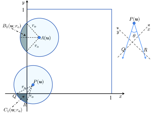
Refer to caption
Figure 1: Illustration of border and corner effects in a unit square.

III Proposed Framework

III-A Boundary Effects

We use the approach suggested in [33] in order to quantify the overlap area |𝒪(𝒖;ro)|𝒪𝒖subscript𝑟o|\mathcal{O}(\boldsymbol{u};r_{\textrm{o}})\cap\mathcal{R}|. The basic building blocks in this approach to characterize the boundary effects are (i) the circular segment areas formed outside each side (border effects) and (ii) the corner overlap areas between two circular segments formed at each vertex (corner effects). We modify the approach in [33] by placing the origin at the vertex V1subscript𝑉1V_{1}, rather than at the center of the square. This leads to a simpler formulation, as discussed below.

Let B1(𝒖;ro)subscript𝐵1𝒖subscript𝑟o{B}_{1}(\boldsymbol{u};r_{\textrm{o}}) denote the area of the circular segment formed outside the side S1subscript𝑆1S_{1}, as illustrated in Fig. 1. Using the fact that the area of the circular segment is equal to the area of the circular sector minus the area of the triangular portion, we obtain

B1(𝒖;ro)={ro2arccos(xro)xro2x2Δs(𝒖,S1)=xro,0otherwise,subscript𝐵1𝒖subscript𝑟ocaseslimit-fromsuperscriptsubscript𝑟o2𝑥subscript𝑟ootherwise𝑥superscriptsubscript𝑟o2superscript𝑥2subscriptΔ𝑠𝒖subscript𝑆1𝑥subscript𝑟o0otherwise\displaystyle B_{1}(\boldsymbol{u};r_{\textrm{o}})\,=\,\begin{cases}r_{\textrm{o}}^{2}\arccos\left(\frac{x}{r_{\textrm{o}}}\right)-\\ \quad x\sqrt{r_{\textrm{o}}^{2}-x^{2}}&\quad\Delta_{s}(\boldsymbol{u},S_{1})=x\geq r_{\textrm{o}},\\ 0&\textrm{otherwise},\end{cases} (7)

where Δs(𝒖,S)subscriptΔ𝑠𝒖subscript𝑆\Delta_{s}(\boldsymbol{u},S_{\ell}) denotes the Euclidean distance between 𝒖𝒖\boldsymbol{u} and side S,=1,2,3,4formulae-sequencesubscript𝑆1234S_{\ell},\,\ell=1,2,3,4. Similarly, the areas of the circular segments formed outside the sides S2subscript𝑆2S_{2}, S3subscript𝑆3S_{3} and S4subscript𝑆4S_{4}, respectively, can be expressed as

B2(𝒖;ro)subscript𝐵2𝒖subscript𝑟o\displaystyle B_{2}(\boldsymbol{u};r_{\textrm{o}})\, ={ro2arccos(yro)yro2y2,Δs(𝒖,S2)=yro0,otherwise,absentcasessuperscriptsubscript𝑟o2𝑦subscript𝑟o𝑦superscriptsubscript𝑟o2superscript𝑦2subscriptΔ𝑠𝒖subscript𝑆2𝑦subscript𝑟o0otherwise\displaystyle=\,\begin{cases}r_{\textrm{o}}^{2}\arccos\left(\frac{y}{r_{\textrm{o}}}\right)-y\sqrt{r_{\textrm{o}}^{2}-y^{2}},&\quad\Delta_{s}(\boldsymbol{u},S_{2})=y\geq r_{\textrm{o}}\\ 0,&\textrm{otherwise},\end{cases} (8)
B3(𝒖;ro)subscript𝐵3𝒖subscript𝑟o\displaystyle B_{3}(\boldsymbol{u};r_{\textrm{o}})\, ={ro2arccos(1xro)(1x)ro2(1x)2,Δs(𝒖,S3)=1xro0,otherwise,absentcasessuperscriptsubscript𝑟o21𝑥subscript𝑟o1𝑥superscriptsubscript𝑟o2superscript1𝑥2subscriptΔ𝑠𝒖subscript𝑆31𝑥subscript𝑟o0otherwise\displaystyle=\,\begin{cases}r_{\textrm{o}}^{2}\arccos\left(\frac{1-x}{r_{\textrm{o}}}\right)-(1-x)\sqrt{r_{\textrm{o}}^{2}-(1-x)^{2}},&\quad\Delta_{s}(\boldsymbol{u},S_{3})=1-x\geq r_{\textrm{o}}\\ 0,&\textrm{otherwise},\end{cases} (9)
B4(𝒖;ro)subscript𝐵4𝒖subscript𝑟o\displaystyle B_{4}(\boldsymbol{u};r_{\textrm{o}})\, ={ro2arccos(1yro)(1y)ro2(1y)2,Δs(𝒖,S4)=1yro0,otherwise.absentcasessuperscriptsubscript𝑟o21𝑦subscript𝑟o1𝑦superscriptsubscript𝑟o2superscript1𝑦2subscriptΔ𝑠𝒖subscript𝑆41𝑦subscript𝑟o0otherwise\displaystyle=\,\begin{cases}r_{\textrm{o}}^{2}\arccos\left(\frac{1-y}{r_{\textrm{o}}}\right)-(1-y)\sqrt{r_{\textrm{o}}^{2}-(1-y)^{2}},&\quad\Delta_{s}(\boldsymbol{u},S_{4})=1-y\geq r_{\textrm{o}}\\ 0,&\textrm{otherwise}.\end{cases} (10)

Let C1(𝒖;ro)subscript𝐶1𝒖subscript𝑟o{C}_{1}(\boldsymbol{u};r_{\textrm{o}}) denote the area of the corner overlap region between two circular segments at vertex V1subscript𝑉1V_{1}, as illustrated in Fig. 1. Using the fact that the area of the overlap region is equal to the area of the circular sector minus the area of two triangular portions, we can easily show that

C1(𝒖;ro)subscript𝐶1𝒖subscript𝑟o\displaystyle C_{1}(\boldsymbol{u};r_{\textrm{o}})\, =12ro2θ12(ro2y2x)y12(ro2x2y)x,absent12superscriptsubscript𝑟o2𝜃12superscriptsubscript𝑟o2superscript𝑦2𝑥𝑦12superscriptsubscript𝑟o2superscript𝑥2𝑦𝑥\displaystyle=\,\frac{1}{2}r_{\textrm{o}}^{2}\theta-\frac{1}{2}\left(\sqrt{r_{\textrm{o}}^{2}-y^{2}}-x\right)y-\frac{1}{2}\left(\sqrt{r_{\textrm{o}}^{2}-x^{2}}-y\right)x, (11)

where the angle θ𝜃\theta is given by

θ𝜃\displaystyle\theta\, = 2arcsin(abs(θ1)2ro),absent2abssubscript𝜃12subscript𝑟o\displaystyle=\,2\arcsin\left(\frac{\mathrm{abs}\left(\sqrt{\theta_{1}}\,\right)}{2r_{\textrm{o}}}\right), (12)

where abs()abs\mathrm{abs}(\cdot) denotes the absolute value or modulus and θ1=2ro22xro2y22yro2x2subscript𝜃12superscriptsubscript𝑟o22𝑥superscriptsubscript𝑟o2superscript𝑦22𝑦superscriptsubscript𝑟o2superscript𝑥2\theta_{1}=2r_{\textrm{o}}^{2}-2x\sqrt{r_{\textrm{o}}^{2}-y^{2}}-2y\sqrt{r_{\textrm{o}}^{2}-x^{2}}. Similarly, the areas of the corner overlap region formed at vertex V2subscript𝑉2V_{2}, V3subscript𝑉3V_{3} and V4subscript𝑉4V_{4}, respectively, can be expressed as

C2(𝒖;ro)subscript𝐶2𝒖subscript𝑟o\displaystyle C_{2}(\boldsymbol{u};r_{\textrm{o}})\, =12ro2α12(ro2y2(1x))y12(ro2(1x)2y)(1x),absent12superscriptsubscript𝑟o2𝛼12superscriptsubscript𝑟o2superscript𝑦21𝑥𝑦12superscriptsubscript𝑟o2superscript1𝑥2𝑦1𝑥\displaystyle=\,\frac{1}{2}r_{\textrm{o}}^{2}\alpha-\frac{1}{2}\left(\sqrt{r_{\textrm{o}}^{2}-y^{2}}-(1-x)\right)y-\frac{1}{2}\left(\sqrt{r_{\textrm{o}}^{2}-(1-x)^{2}}-y\right)(1-x), (13)
C3(𝒖;ro)subscript𝐶3𝒖subscript𝑟o\displaystyle C_{3}(\boldsymbol{u};r_{\textrm{o}})\, =12ro2β12(ro2(1y)2(1x))(1y)12(ro2(1x)2(1y))(1x),absent12superscriptsubscript𝑟o2𝛽12superscriptsubscript𝑟o2superscript1𝑦21𝑥1𝑦12superscriptsubscript𝑟o2superscript1𝑥21𝑦1𝑥\displaystyle=\,\frac{1}{2}r_{\textrm{o}}^{2}\beta-\frac{1}{2}\left(\sqrt{r_{\textrm{o}}^{2}-(1-y)^{2}}-(1-x)\right)(1-y)-\frac{1}{2}\left(\sqrt{r_{\textrm{o}}^{2}-(1-x)^{2}}-(1-y)\right)(1-x), (14)
C4(𝒖;ro)subscript𝐶4𝒖subscript𝑟o\displaystyle C_{4}(\boldsymbol{u};r_{\textrm{o}})\, =12ro2γ12(ro2(1y)2x)(1y)12(ro2x2(1y))x,absent12superscriptsubscript𝑟o2𝛾12superscriptsubscript𝑟o2superscript1𝑦2𝑥1𝑦12superscriptsubscript𝑟o2superscript𝑥21𝑦𝑥\displaystyle=\,\frac{1}{2}r_{\textrm{o}}^{2}\gamma-\frac{1}{2}\left(\sqrt{r_{\textrm{o}}^{2}-(1-y)^{2}}-x\right)(1-y)-\frac{1}{2}\left(\sqrt{r_{\textrm{o}}^{2}-x^{2}}-(1-y)\right)x, (15)

where the angles α𝛼\alpha, β𝛽\beta and γ𝛾\gamma are given by

α𝛼\displaystyle\alpha\, = 2arcsin(abs(α1)2ro)absent2abssubscript𝛼12subscript𝑟o\displaystyle=\,2\arcsin\left(\frac{\mathrm{abs}\left(\sqrt{\alpha_{1}}\right)}{2r_{\textrm{o}}}\right) (16)
β𝛽\displaystyle\beta\, = 2arcsin(abs(β1)2ro)absent2abssubscript𝛽12subscript𝑟o\displaystyle=\,2\arcsin\left(\frac{\mathrm{abs}\left(\sqrt{\beta_{1}}\right)}{2r_{\textrm{o}}}\right) (17)
γ𝛾\displaystyle\gamma\, = 2arcsin(abs(γ1)2ro)absent2abssubscript𝛾12subscript𝑟o\displaystyle=\,2\arcsin\left(\frac{\mathrm{abs}\left(\sqrt{\gamma_{1}}\right)}{2r_{\textrm{o}}}\right) (18)

where α1=2ro22(1x)ro2y22yro2(1x)2subscript𝛼12superscriptsubscript𝑟o221𝑥superscriptsubscript𝑟o2superscript𝑦22𝑦superscriptsubscript𝑟o2superscript1𝑥2\alpha_{1}=2r_{\textrm{o}}^{2}-2(1-x)\sqrt{r_{\textrm{o}}^{2}-y^{2}}-2y\sqrt{r_{\textrm{o}}^{2}-(1-x)^{2}}, β1=2ro22(1x)ro2(1y)22(1y)ro2(1x)2subscript𝛽12superscriptsubscript𝑟o221𝑥superscriptsubscript𝑟o2superscript1𝑦221𝑦superscriptsubscript𝑟o2superscript1𝑥2\beta_{1}=2r_{\textrm{o}}^{2}-2(1-x)\sqrt{r_{\textrm{o}}^{2}-(1-y)^{2}}-2(1-y)\sqrt{r_{\textrm{o}}^{2}-(1-x)^{2}} and γ1=2ro22xro2(1y)22(1y)ro2x2subscript𝛾12superscriptsubscript𝑟o22𝑥superscriptsubscript𝑟o2superscript1𝑦221𝑦superscriptsubscript𝑟o2superscript𝑥2\gamma_{1}=2r_{\textrm{o}}^{2}-2x\sqrt{r_{\textrm{o}}^{2}-(1-y)^{2}}-2(1-y)\sqrt{r_{\textrm{o}}^{2}-x^{2}}. We note that the expressions for C(𝒖;ro)subscript𝐶𝒖subscript𝑟oC_{\ell}(\boldsymbol{u};r_{\textrm{o}}) are valid only when Δs(𝒖,V)rosubscriptΔ𝑠𝒖subscript𝑉subscript𝑟o\Delta_{s}(\boldsymbol{u},V_{\ell})\geq r_{\textrm{o}}, where Δs(𝒖,V)subscriptΔ𝑠𝒖subscript𝑉\Delta_{s}(\boldsymbol{u},V_{\ell}) denotes the Euclidean distance between 𝒖𝒖\boldsymbol{u} and vertex V,=1,2,3,4formulae-sequencesubscript𝑉1234V_{\ell},\,\ell=1,2,3,4.. For the case when Δs(𝒖,V)<rosubscriptΔ𝑠𝒖subscript𝑉subscript𝑟o\Delta_{s}(\boldsymbol{u},V_{\ell})<r_{\textrm{o}}, C(𝒖;ro)=0subscript𝐶𝒖subscript𝑟o0C_{\ell}(\boldsymbol{u};r_{\textrm{o}})=0.

Using (7)-(10) and (11),absent,~{}(13)-(15), the CDF F(𝒖;ro)𝐹𝒖subscript𝑟oF(\boldsymbol{u};r_{\textrm{o}}) in (3) can be expressed in closed-form, e.g., if ro=0.1subscript𝑟o0.1r_{\textrm{o}}=0.1 and 𝒖=(0,0)𝒖00\boldsymbol{u}=(0,0), then two circular segments are formed outside sides S1subscript𝑆1S_{1} and S2subscript𝑆2S_{2} and also there is overlap between them. Hence, in this case, F(𝒖;ro)=πro2(B1(𝒖;ro)+B2(𝒖;ro)C1(𝒖;ro))𝐹𝒖subscript𝑟o𝜋superscriptsubscript𝑟o2subscript𝐵1𝒖subscript𝑟osubscript𝐵2𝒖subscript𝑟osubscript𝐶1𝒖subscript𝑟oF(\boldsymbol{u};r_{\textrm{o}})=\pi r_{\textrm{o}}^{2}-(B_{1}(\boldsymbol{u};r_{\textrm{o}})+B_{2}(\boldsymbol{u};r_{\textrm{o}})-C_{1}(\boldsymbol{u};r_{\textrm{o}})). This will be further illustrated in the next subsection.

III-B Tractable Framework

As illustrated in the last subsection, for a given value of the transmission range rosubscript𝑟or_{\textrm{o}} and the location of the arbitrary node 𝒖𝒖\boldsymbol{u}, F(𝒖;ro)𝐹𝒖subscript𝑟oF(\boldsymbol{u};r_{\textrm{o}}) can be expressed in closed-form using (7)-(10) and (11),absent,~{}(13)-(15). In order to facilitate the averaging of (3) over the whole square region, we divide the square region into different non-overlapping subregions based on the different border and corner effects that occur in that region. Due to the symmetry of the square, some subregions have the same number of border and corner effects which can be exploited to further simplify the averaging. This will be elaborated in detail shortly.

Let 1subscript1\mathcal{R}_{1}, 2subscript2\mathcal{R}_{2}, \ldots Msubscript𝑀\mathcal{R}_{M} denote the type of non-overlapping subregions and nisubscript𝑛𝑖n_{i}, i{1, 2,M}𝑖12𝑀i\in\{1,\,2\,\ldots,\,M\} denote the number of subregion of type isubscript𝑖\mathcal{R}_{i}. If Fi(𝒖;ro)subscript𝐹𝑖𝒖subscript𝑟oF_{i}(\boldsymbol{u};r_{\textrm{o}}) denotes the conditional probability of connectivity for a node located at 𝒖i𝒖subscript𝑖\boldsymbol{u}\in\mathcal{R}_{i}, we can write the probability of node isolation in (2) as

Piso(ro)=i=1Mnii(1Fi(𝒖;ro))N1𝑑s(𝒖),subscript𝑃isosubscript𝑟osuperscriptsubscript𝑖1𝑀subscript𝑛𝑖subscriptsubscript𝑖superscript1subscript𝐹𝑖𝒖subscript𝑟o𝑁1differential-d𝑠𝒖\displaystyle P_{\textrm{iso}}(r_{\textrm{o}})\,=\,\sum_{i=1}^{M}n_{i}\,\displaystyle\int_{\mathcal{R}_{i}}\big{(}1-F_{i}(\boldsymbol{u};r_{\textrm{o}})\big{)}^{N-1}ds(\boldsymbol{u}), (19)

and the minimum node degree distribution fD(k;ro)subscript𝑓𝐷𝑘subscript𝑟of_{D}(k;r_{\textrm{o}}) in (3) as

fD(k;ro)subscript𝑓𝐷𝑘subscript𝑟o\displaystyle f_{D}(k;r_{\textrm{o}}) =P(D=k)=(1d=0k1i=1Mni(N1d)×\displaystyle=\textrm{P}(D=k)=\bigg{(}1-\sum_{d=0}^{k-1}\sum_{i=1}^{M}n_{i}\binom{N-1}{d}\,\times
i(F(𝒖;ro))d(1F(𝒖;ro))nd1ds(𝒖))N.\displaystyle\displaystyle\int_{\mathcal{R}_{i}}\left(F(\boldsymbol{u};r_{\textrm{o}})\right)^{d}\left(1-F(\boldsymbol{u};r_{\textrm{o}})\right)^{n-d-1}ds(\boldsymbol{u})\bigg{)}^{N}. (20)

We note that the average node degree denoted by D¯¯𝐷\overline{D} can also be determined using our framework as [14]

D¯¯𝐷\displaystyle\overline{D} =(N1)F(𝒖;ro)𝑑s(𝒖)absent𝑁1subscript𝐹𝒖subscript𝑟odifferential-d𝑠𝒖\displaystyle=(N-1)\int_{\mathcal{R}}F(\boldsymbol{u};r_{\textrm{o}})ds(\boldsymbol{u})
=(N1)i=1MniiF(𝒖;ro)𝑑s(𝒖).absent𝑁1superscriptsubscript𝑖1𝑀subscript𝑛𝑖subscriptsubscript𝑖𝐹𝒖subscript𝑟odifferential-d𝑠𝒖\displaystyle=(N-1)\sum_{i=1}^{M}n_{i}\,\displaystyle\int_{\mathcal{R}_{i}}F(\boldsymbol{u};r_{\textrm{o}})ds(\boldsymbol{u}). (21)

In fact F(𝒖;ro)𝑑s(𝒖)subscript𝐹𝒖subscript𝑟odifferential-d𝑠𝒖\int_{\mathcal{R}}F(\boldsymbol{u};r_{\textrm{o}})ds(\boldsymbol{u}) in (III-B) denotes the cumulative distribution function of the distance between two randomly placed nodes and the closed form analytical results exist in the literature for square, hexagon [6] and convex regular polygons [34].

Remark 1

The general formulation for Piso(ro)subscript𝑃isosubscript𝑟oP_{\textrm{iso}}(r_{\textrm{o}}) in (2) is also indirectly suggested in [25]. However, no guidelines are presented in order to evaluate (2). Hence, the authors in [25] use a deterministic grid deployment of nodes to approximate the boundary effects when nodes are uniformly and independently distributed in a square region. By contrast, we provide a tractable framework for complete and exact characterization of the boundary effects in (19).

Remark 2

While Fi(𝐮;ro)subscript𝐹𝑖𝐮subscript𝑟oF_{i}(\boldsymbol{u};r_{\textrm{o}}) in (3) can be expressed analytically in closed-form, the integration in (19) and (III-B) does not have a closed-form due to the N1𝑁1N-1 factor in the exponent. However, it can be easily evaluated numerically using the explicit closed-form expressions for Fi(𝐮;ro)subscript𝐹𝑖𝐮subscript𝑟oF_{i}(\boldsymbol{u};r_{\textrm{o}}) for different transmission ranges and different subregions. It must be noted that numerical evaluation of two-fold integrals is widely practiced in the literature [35].

Remark 3

We have considered a unit square region for the sake of simplicity in the proposed formulation. For the general case of a square of side length L𝐿L, (19)-(III-B) can be used with appropriate scaling of the transmission range as roro/Lsubscript𝑟osubscript𝑟o𝐿r_{\textrm{o}}\rightarrow r_{\textrm{o}}/L.

Since the subregions are classified on the basis of the boundary effects, the subregions change with the transmission range rosubscript𝑟or_{\textrm{o}}. We divide the range rosubscript𝑟or_{\textrm{o}} over the desired interval 0ro20subscript𝑟o20\leq r_{\textrm{o}}\leq\sqrt{2}, as explained in Section II-C, such that the boundary effects are the same for the different subregions over each subinterval of the transmission range. This is explained in detail in the next section.

IV Effect of Boundaries for the Different Transmission Range Cases

IV-A Transmission Range - 0ro1/20subscript𝑟o120\leq r_{\textrm{o}}\leq 1/2

Consider the first case of the transmission range, i.e., 0ro120subscript𝑟o120\leq r_{\textrm{o}}\leq\frac{1}{2}, as shown in Fig. 3. This case may be of greatest interest in many practical situations where typically the sensor transmission range is a small fraction of the side length of the square. In this case, we can divide the square into four (M=4𝑀4M=4) types of subregions 1subscript1\mathcal{R}_{1}, 2subscript2\mathcal{R}_{2}, 3subscript3\mathcal{R}_{3} and 4subscript4\mathcal{R}_{4}. As shown in Fig. 3, although there is one subregion of type 1subscript1\mathcal{R}_{1}, there are four subregions of types 2subscript2\mathcal{R}_{2}, 3subscript3\mathcal{R}_{3} and 4subscript4\mathcal{R}_{4}, respectively, which are shaded in the same color for ease of identification, e.g., for an arbitrary node located in any subregion of type 2subscript2\mathcal{R}_{2}, the disk 𝒪(𝒖;ro)𝒪𝒖subscript𝑟o\mathcal{O}(\boldsymbol{u};r_{\textrm{o}}) is limited by one side only. Hence, we determine Fi(𝒖;ro)subscript𝐹𝑖𝒖subscript𝑟oF_{i}(\boldsymbol{u};r_{\textrm{o}}) only for the following subregions

  • 1={x(ro,1ro),y(ro,1ro)}subscript1formulae-sequence𝑥subscript𝑟o1subscript𝑟o𝑦subscript𝑟o1subscript𝑟o\mathcal{R}_{1}=\{x\in(r_{\textrm{o}},1-r_{\textrm{o}}),\,y\in(r_{\textrm{o}},1-r_{\textrm{o}})\}

  • 2={x(0,ro),y(ro,1ro)}subscript2formulae-sequence𝑥0subscript𝑟o𝑦subscript𝑟o1subscript𝑟o\mathcal{R}_{2}=\{x\in(0,r_{\textrm{o}}),\,y\in(r_{\textrm{o}},1-r_{\textrm{o}})\}

  • 3={x(0,ro),y(ro2x2,ro)}subscript3formulae-sequence𝑥0subscript𝑟o𝑦superscriptsubscript𝑟o2superscript𝑥2subscript𝑟o\mathcal{R}_{3}=\{x\in(0,r_{\textrm{o}}),\,y\in(\sqrt{r_{\textrm{o}}^{2}-x^{2}},r_{\textrm{o}})\}

  • 4={x(0,ro),y(0,ro2x2)}subscript4formulae-sequence𝑥0subscript𝑟o𝑦0superscriptsubscript𝑟o2superscript𝑥2\mathcal{R}_{4}=\{x\in(0,r_{\textrm{o}}),\,y\in(0,\sqrt{r_{\textrm{o}}^{2}-x^{2}})\}

Figure 2: *

Subregions [Uncaptioned image]

TABLE I:
isubscript𝑖\mathcal{R}_{i} nisubscript𝑛𝑖n_{i} Fi(𝒖;ro)subscript𝐹𝑖𝒖subscript𝑟oF_{i}(\boldsymbol{u};r_{\textrm{o}})
1subscript1\mathcal{R}_{1} 111 πro2𝜋superscriptsubscript𝑟o2\pi r_{\textrm{o}}^{2}
2subscript2\mathcal{R}_{2} 444 πro2(B1)𝜋superscriptsubscript𝑟o2subscript𝐵1\pi r_{\textrm{o}}^{2}-(B_{1})
3subscript3\mathcal{R}_{3} 444 πro2(B1+B2)𝜋superscriptsubscript𝑟o2subscript𝐵1subscript𝐵2\pi r_{\textrm{o}}^{2}-(B_{1}+B_{2})
4subscript4\mathcal{R}_{4} 444 πro2(B1+B2C1)𝜋superscriptsubscript𝑟o2subscript𝐵1subscript𝐵2subscript𝐶1\pi r_{\textrm{o}}^{2}-(B_{1}+B_{2}-C_{1})
Figure 3: Subregions for transmission range 0ro120subscript𝑟o120\leq r_{\textrm{o}}\leq\frac{1}{2} are shown in the figure (top) and conditional probabilities Fi(𝒖;ro)subscript𝐹𝑖𝒖subscript𝑟oF_{i}(\boldsymbol{u};r_{\textrm{o}}) and number of subregions nisubscript𝑛𝑖n_{i} for each subregion are shown in the Table I (bottom).

It is easy to see that for an arbitrary node located anywhere in subregion 1subscript1\mathcal{R}_{1}, the disk 𝒪(𝒖;ro)𝒪𝒖subscript𝑟o\mathcal{O}(\boldsymbol{u};r_{\textrm{o}}) is completely inside the square \mathcal{R}, i.e., there are no border or corner effects. Hence, F1(𝒖;ro)=πro2subscript𝐹1𝒖subscript𝑟o𝜋superscriptsubscript𝑟o2F_{1}(\boldsymbol{u};r_{\textrm{o}})=\pi r_{\textrm{o}}^{2}. For an arbitrary node located anywhere in subregion 2subscript2\mathcal{R}_{2}, the disk 𝒪(𝒖;ro)𝒪𝒖subscript𝑟o\mathcal{O}(\boldsymbol{u};r_{\textrm{o}}) is limited by side S1subscript𝑆1S_{1}, i.e., there is a circular segment formed outside the side S1subscript𝑆1S_{1}. Hence, F2(𝒖;ro)=πro2(B1(𝒖;ro))subscript𝐹2𝒖subscript𝑟o𝜋superscriptsubscript𝑟o2subscript𝐵1𝒖subscript𝑟oF_{2}(\boldsymbol{u};r_{\textrm{o}})=\pi r_{\textrm{o}}^{2}-(B_{1}(\boldsymbol{u};r_{\textrm{o}})). For an arbitrary node located anywhere in subregion 3subscript3\mathcal{R}_{3}, the disk 𝒪(𝒖;ro)𝒪𝒖subscript𝑟o\mathcal{O}(\boldsymbol{u};r_{\textrm{o}}) is limited by sides S1subscript𝑆1S_{1} and S2subscript𝑆2S_{2}, i.e., there is are two circular segments formed outside the sides S1subscript𝑆1S_{1} and S2subscript𝑆2S_{2} and there is no corner overlap between them. Hence, F3(𝒖;ro)=πro2(B1(𝒖;ro)+B2(𝒖;ro))subscript𝐹3𝒖subscript𝑟o𝜋superscriptsubscript𝑟o2subscript𝐵1𝒖subscript𝑟osubscript𝐵2𝒖subscript𝑟oF_{3}(\boldsymbol{u};r_{\textrm{o}})=\pi r_{\textrm{o}}^{2}-(B_{1}(\boldsymbol{u};r_{\textrm{o}})+B_{2}(\boldsymbol{u};r_{\textrm{o}})). For an arbitrary node located anywhere in subregion 4subscript4\mathcal{R}_{4}, the disk 𝒪(𝒖;ro)𝒪𝒖subscript𝑟o\mathcal{O}(\boldsymbol{u};r_{\textrm{o}}) is limited by sides S1subscript𝑆1S_{1} and S2subscript𝑆2S_{2} and vertex V1subscript𝑉1V_{1}, i.e., there is are two circular segments formed outside the sides S1subscript𝑆1S_{1} and S2subscript𝑆2S_{2} and there is corner overlap between them. Hence, F4(𝒖;ro)=πro2(B1(𝒖;ro)+B2(𝒖;ro)C1(𝒖;ro))subscript𝐹4𝒖subscript𝑟o𝜋superscriptsubscript𝑟o2subscript𝐵1𝒖subscript𝑟osubscript𝐵2𝒖subscript𝑟osubscript𝐶1𝒖subscript𝑟oF_{4}(\boldsymbol{u};r_{\textrm{o}})=\pi r_{\textrm{o}}^{2}-(B_{1}(\boldsymbol{u};r_{\textrm{o}})+B_{2}(\boldsymbol{u};r_{\textrm{o}})-C_{1}(\boldsymbol{u};r_{\textrm{o}})). The number of subregions nisubscript𝑛𝑖n_{i} of each type and the corresponding closed form Fi(𝒖;ro)subscript𝐹𝑖𝒖subscript𝑟oF_{i}(\boldsymbol{u};r_{\textrm{o}}) are tabulated in Table I. For the sake of brevity, B(u;r0)subscript𝐵𝑢subscript𝑟0B_{\ell}(u;r_{0}) and C(u;r0)subscript𝐶𝑢subscript𝑟0C_{\ell}(u;r_{0}) are denoted as Bsubscript𝐵B_{\ell} and Csubscript𝐶C_{\ell}, respectively in this and subsequent tables.

As rosubscript𝑟or_{\textrm{o}} increases from 00 to 1/212{1}/{2}, we can see that the subregions of type 1subscript1\mathcal{R}_{1} and 2subscript2\mathcal{R}_{2} become smaller and the subregions of type 3subscript3\mathcal{R}_{3} and 4subscript4\mathcal{R}_{4} become larger. For the value of range ro=12subscript𝑟o12r_{\textrm{o}}=\frac{1}{2}, the subregions of type 1subscript1\mathcal{R}_{1} and 2subscript2\mathcal{R}_{2} approach zero.

Remark 4

The division of the square \mathcal{R} into subregions for transmission range 0ro1/20subscript𝑟o120\leq r_{\textrm{o}}\leq 1/2 has been previously shown in [25, Fig. 7], [26, Fig. 2] and [29, Fig. 2] to illustrate the intuitive argument that the nodes situated in boundary subregions experience border effects. However, subregions 3subscript3\mathcal{R}_{3} and 4subscript4\mathcal{R}_{4} are indicated as one subregion in [26, 25]. Using our framework, we show that these are two distinct subregions with unique border and corner effects. In addition, we formulate all the subregions for all possible values of the range. This is different to [29, 36] where only the transmission range 0ro1/20subscript𝑟o120\leq r_{\textrm{o}}\leq 1/2 was considered for finding the average node degree.

IV-B Transmission Range - 1/2ro(22)12subscript𝑟o221/2\leq r_{\textrm{o}}\leq(2-\sqrt{2})

For the case of the transmission range in the interval 1/2ro2212subscript𝑟o221/2\leq r_{\textrm{o}}\leq 2-\sqrt{2}, we have M=6𝑀6M=6 types of subregions, which are shown in Fig. 5 and can be expressed as

  • 1={x(0,2ro1),y(0,1ro)}{x(2ro1,1ro),y(0,ro2x2)}subscript1formulae-sequence𝑥02subscript𝑟o1𝑦01subscript𝑟oformulae-sequence𝑥2subscript𝑟o11subscript𝑟o𝑦0superscriptsubscript𝑟o2superscript𝑥2\mathcal{R}_{1}=\{x\in(0,\sqrt{2r_{\textrm{o}}-1}),\,y\in(0,1-r_{\textrm{o}})\}\cup\{x\in(\sqrt{2r_{\textrm{o}}-1},1-r_{\textrm{o}}),\,y\in(0,\sqrt{r_{\textrm{o}}^{2}-x^{2}})\}

  • 2={x(1ro,0.5),y(0,ro2(x1)2)}subscript2formulae-sequence𝑥1subscript𝑟o0.5𝑦0superscriptsubscript𝑟o2superscript𝑥12\mathcal{R}_{2}=\{x\in(1-r_{\textrm{o}},0.5),\,y\in(0,\sqrt{r_{\textrm{o}}^{2}-(x-1)^{2}})\}

  • 3={x(1ro,0.5),y(ro2(x1)2,ro2x2)}subscript3formulae-sequence𝑥1subscript𝑟o0.5𝑦superscriptsubscript𝑟o2superscript𝑥12superscriptsubscript𝑟o2superscript𝑥2\mathcal{R}_{3}=\{x\in(1-r_{\textrm{o}},0.5),\,y\in(\sqrt{r_{\textrm{o}}^{2}-(x-1)^{2}},\sqrt{r_{\textrm{o}}^{2}-x^{2}})\}

  • 4={x(1ro,0.5),y(ro2x2,1ro)}subscript4formulae-sequence𝑥1subscript𝑟o0.5𝑦superscriptsubscript𝑟o2superscript𝑥21subscript𝑟o\mathcal{R}_{4}=\{x\in(1-r_{\textrm{o}},0.5),\,y\in(\sqrt{r_{\textrm{o}}^{2}-x^{2}},1-r_{\textrm{o}})\}

  • 5={x(2ro1,1ro),y(ro2x2,1ro)}subscript5formulae-sequence𝑥2subscript𝑟o11subscript𝑟o𝑦superscriptsubscript𝑟o2superscript𝑥21subscript𝑟o\mathcal{R}_{5}=\{x\in(\sqrt{2r_{\textrm{o}}-1},1-r_{\textrm{o}}),\,y\in(\sqrt{r_{\textrm{o}}^{2}-x^{2}},1-r_{\textrm{o}})\}

  • 6={x(1ro,0.5),y(1ro,0.5)}subscript6formulae-sequence𝑥1subscript𝑟o0.5𝑦1subscript𝑟o0.5\mathcal{R}_{6}=\{x\in(1-r_{\textrm{o}},0.5),\,y\in(1-r_{\textrm{o}},0.5)\}

Figure 4: *

Subregions [Uncaptioned image]

TABLE II:
isubscript𝑖\mathcal{R}_{i} nisubscript𝑛𝑖n_{i} Fi(𝒖;ro)subscript𝐹𝑖𝒖subscript𝑟oF_{i}(\boldsymbol{u};r_{\textrm{o}})
1subscript1\mathcal{R}_{1} 444 πro2(B1+B2C1)𝜋superscriptsubscript𝑟o2subscript𝐵1subscript𝐵2subscript𝐶1\pi r_{\textrm{o}}^{2}-(B_{1}+B_{2}-C_{1})
2subscript2\mathcal{R}_{2} 888 πro2(B1+B2+B3C1C2)𝜋superscriptsubscript𝑟o2subscript𝐵1subscript𝐵2subscript𝐵3subscript𝐶1subscript𝐶2\pi r_{\textrm{o}}^{2}-(B_{1}+B_{2}+B_{3}-C_{1}-C_{2})
3subscript3\mathcal{R}_{3} 888 πro2(B1+B2+B3C1)𝜋superscriptsubscript𝑟o2subscript𝐵1subscript𝐵2subscript𝐵3subscript𝐶1\pi r_{\textrm{o}}^{2}-(B_{1}+B_{2}+B_{3}-C_{1})
4subscript4\mathcal{R}_{4} 888 πro2(B1+B2+B3)𝜋superscriptsubscript𝑟o2subscript𝐵1subscript𝐵2subscript𝐵3\pi r_{\textrm{o}}^{2}-(B_{1}+B_{2}+B_{3})
5subscript5\mathcal{R}_{5} 444 πro2(B1+B2)𝜋superscriptsubscript𝑟o2subscript𝐵1subscript𝐵2\pi r_{\textrm{o}}^{2}-(B_{1}+B_{2})
6subscript6\mathcal{R}_{6} 444 πro2(B1+B2+B3+B4)𝜋superscriptsubscript𝑟o2subscript𝐵1subscript𝐵2subscript𝐵3subscript𝐵4\pi r_{\textrm{o}}^{2}-(B_{1}+B_{2}+B_{3}+B_{4})
Figure 5: Subregions for transmission range 1/2ro(22)12subscript𝑟o221/2\leq r_{\textrm{o}}\leq(2-\sqrt{2}) are shown in the figure (top) and conditional probabilities Fi(𝒖;ro)subscript𝐹𝑖𝒖subscript𝑟oF_{i}(\boldsymbol{u};r_{\textrm{o}}) and number of subregions nisubscript𝑛𝑖n_{i} for each subregion are shown in the Table II (bottom).

The upper limit for this interval of transmission range, i.e., (22)22(2-\sqrt{2}) is computed as the range rosubscript𝑟or_{\textrm{o}} for which the lines x=1ro𝑥1subscript𝑟ox=1-r_{\textrm{o}}, y=1ro𝑦1subscript𝑟oy=1-r_{\textrm{o}} and circle x2+y2=ro2superscript𝑥2superscript𝑦2superscriptsubscript𝑟o2x^{2}+y^{2}=r_{\textrm{o}}^{2} intersect. As rosubscript𝑟or_{\textrm{o}} approaches (22)22(2-\sqrt{2}), the subregion 5subscript5\mathcal{R}_{5} squeezes to zero. The number of subregions nisubscript𝑛𝑖n_{i} of each type and the corresponding closed-form Fi(𝒖;ro)subscript𝐹𝑖𝒖subscript𝑟oF_{i}(\boldsymbol{u};r_{\textrm{o}}) are tabulated in Table II.

Figure 6: *

Subregions [Uncaptioned image]

TABLE III:
isubscript𝑖\mathcal{R}_{i} nisubscript𝑛𝑖n_{i} Fi(𝒖;ro)subscript𝐹𝑖𝒖subscript𝑟oF_{i}(\boldsymbol{u};r_{\textrm{o}})
1subscript1\mathcal{R}_{1} 444 πro2(B1+B2C1)𝜋superscriptsubscript𝑟o2subscript𝐵1subscript𝐵2subscript𝐶1\pi r_{\textrm{o}}^{2}-(B_{1}+B_{2}-C_{1})
2subscript2\mathcal{R}_{2} 888 πro2(B1+B2+B3C1C2)𝜋superscriptsubscript𝑟o2subscript𝐵1subscript𝐵2subscript𝐵3subscript𝐶1subscript𝐶2\pi r_{\textrm{o}}^{2}-(B_{1}+B_{2}+B_{3}-C_{1}-C_{2})
3subscript3\mathcal{R}_{3} 888 πro2(B1+B2+B3C1)𝜋superscriptsubscript𝑟o2subscript𝐵1subscript𝐵2subscript𝐵3subscript𝐶1\pi r_{\textrm{o}}^{2}-(B_{1}+B_{2}+B_{3}-C_{1})
4subscript4\mathcal{R}_{4} 888 πro2(B1+B2+B3)𝜋superscriptsubscript𝑟o2subscript𝐵1subscript𝐵2subscript𝐵3\pi r_{\textrm{o}}^{2}-(B_{1}+B_{2}+B_{3})
5subscript5\mathcal{R}_{5} 444 πro2(B1+B2+B3+B4C1)𝜋superscriptsubscript𝑟o2subscript𝐵1subscript𝐵2subscript𝐵3subscript𝐵4subscript𝐶1\pi r_{\textrm{o}}^{2}-(B_{1}+B_{2}+B_{3}+B_{4}-C_{1})
6subscript6\mathcal{R}_{6} 444 πro2(B1+B2+B3+B4)𝜋superscriptsubscript𝑟o2subscript𝐵1subscript𝐵2subscript𝐵3subscript𝐵4\pi r_{\textrm{o}}^{2}-(B_{1}+B_{2}+B_{3}+B_{4})
Figure 7: Subregions for transmission range (22)ro5/822subscript𝑟o58(2-\sqrt{2})\leq r_{\textrm{o}}\leq 5/8 are shown in the figure (top) and conditional probabilities Fi(𝒖;ro)subscript𝐹𝑖𝒖subscript𝑟oF_{i}(\boldsymbol{u};r_{\textrm{o}}) and number of subregions nisubscript𝑛𝑖n_{i} for each subregion are shown in the Table III (bottom).

IV-C Transmission Range - (22)ro5/822subscript𝑟o58(2-\sqrt{2})\leq r_{\textrm{o}}\leq 5/8

For the case of the transmission range in the interval (22)ro5/822subscript𝑟o58(2-\sqrt{2})\leq r_{\textrm{o}}\leq 5/8, we again have M=6𝑀6M=6 types of subregions, which are shown in Fig. 7 and can be expressed as

  • 1={x(0,1ro),y(0,1ro)}subscript1formulae-sequence𝑥01subscript𝑟o𝑦01subscript𝑟o\mathcal{R}_{1}=\{x\in(0,1-r_{\textrm{o}}),\,y\in(0,1-r_{\textrm{o}})\}

  • 2={x(1ro,0.5),y(0,ro2(x1)2)}subscript2formulae-sequence𝑥1subscript𝑟o0.5𝑦0superscriptsubscript𝑟o2superscript𝑥12\mathcal{R}_{2}=\{x\in(1-r_{\textrm{o}},0.5),\,y\in(0,\sqrt{r_{\textrm{o}}^{2}-(x-1)^{2}})\}

  • 3={x(1ro,2ro1),y(ro2(x1)2,1ro)}{x(2ro1,0.5),y(ro2(x1)2,ro2x2)}subscript3formulae-sequence𝑥1subscript𝑟o2subscript𝑟o1𝑦superscriptsubscript𝑟o2superscript𝑥121subscript𝑟oformulae-sequence𝑥2subscript𝑟o10.5𝑦superscriptsubscript𝑟o2superscript𝑥12superscriptsubscript𝑟o2superscript𝑥2\mathcal{R}_{3}=\{x\in(1-r_{\textrm{o}},\sqrt{2r_{\textrm{o}}-1}),\,y\in(\sqrt{r_{\textrm{o}}^{2}-(x-1)^{2}},1-r_{\textrm{o}})\}\cup\{x\in(\sqrt{2r_{\textrm{o}}-1},0.5),\,y\in(\sqrt{r_{\textrm{o}}^{2}-(x-1)^{2}},\sqrt{r_{\textrm{o}}^{2}-x^{2}})\}

  • 4={x(2ro1,0.5),y(ro2x2,1ro)}subscript4formulae-sequence𝑥2subscript𝑟o10.5𝑦superscriptsubscript𝑟o2superscript𝑥21subscript𝑟o\mathcal{R}_{4}=\{x\in(\sqrt{2r_{\textrm{o}}-1},0.5),\,y\in(\sqrt{r_{\textrm{o}}^{2}-x^{2}},1-r_{\textrm{o}})\}

  • 5={x(1ro,2ro1),y(1ro,ro2x2)}subscript5formulae-sequence𝑥1subscript𝑟o2subscript𝑟o1𝑦1subscript𝑟osuperscriptsubscript𝑟o2superscript𝑥2\mathcal{R}_{5}=\{x\in(1-r_{\textrm{o}},\sqrt{2r_{\textrm{o}}-1}),\,y\in(1-r_{\textrm{o}},\sqrt{r_{\textrm{o}}^{2}-x^{2}})\}

  • 6={x(1ro,2ro1),y(ro2x2,0.5)}{x(2ro1,0.5),y(1ro,0.5)}subscript6formulae-sequence𝑥1subscript𝑟o2subscript𝑟o1𝑦superscriptsubscript𝑟o2superscript𝑥20.5formulae-sequence𝑥2subscript𝑟o10.5𝑦1subscript𝑟o0.5\mathcal{R}_{6}=\{x\in(1-r_{\textrm{o}},\sqrt{2r_{\textrm{o}}-1}),\,y\in(\sqrt{r_{\textrm{o}}^{2}-x^{2}},0.5)\}\cup\{x\in(\sqrt{2r_{\textrm{o}}-1},0.5),\,y\in(1-r_{\textrm{o}},0.5)\}

The upper limit for this interval of the transmission range, i.e., 5/8585/8 is determined as the range rosubscript𝑟or_{\textrm{o}} where the subregion 4subscript4\mathcal{R}_{4} squeezes to zero and is computed as an intersection of the line y=1ro𝑦1subscript𝑟oy=1-r_{\textrm{o}} and two circles x2+y2=ro2superscript𝑥2superscript𝑦2superscriptsubscript𝑟o2x^{2}+y^{2}=r_{\textrm{o}}^{2} and (x1)2+y2=ro2superscript𝑥12superscript𝑦2superscriptsubscript𝑟o2(x-1)^{2}+y^{2}=r_{\textrm{o}}^{2}. The number of subregions nisubscript𝑛𝑖n_{i} of each type and the corresponding closed-form Fi(𝒖;ro)subscript𝐹𝑖𝒖subscript𝑟oF_{i}(\boldsymbol{u};r_{\textrm{o}}) are tabulated in Table III.

Figure 8: *

Subregions [Uncaptioned image]

TABLE IV:
isubscript𝑖\mathcal{R}_{i} nisubscript𝑛𝑖n_{i} Fi(𝒖;ro)subscript𝐹𝑖𝒖subscript𝑟oF_{i}(\boldsymbol{u};r_{\textrm{o}})
1subscript1\mathcal{R}_{1} 444 πro2(B1+B2C1)𝜋superscriptsubscript𝑟o2subscript𝐵1subscript𝐵2subscript𝐶1\pi r_{\textrm{o}}^{2}-(B_{1}+B_{2}-C_{1})
2subscript2\mathcal{R}_{2} 888 πro2(B1+B2+B3C1C2)𝜋superscriptsubscript𝑟o2subscript𝐵1subscript𝐵2subscript𝐵3subscript𝐶1subscript𝐶2\pi r_{\textrm{o}}^{2}-(B_{1}+B_{2}+B_{3}-C_{1}-C_{2})
3subscript3\mathcal{R}_{3} 888 πro2(B1+B2+B3C1)𝜋superscriptsubscript𝑟o2subscript𝐵1subscript𝐵2subscript𝐵3subscript𝐶1\pi r_{\textrm{o}}^{2}-(B_{1}+B_{2}+B_{3}-C_{1})
4subscript4\mathcal{R}_{4} 888 πro2(B1+B2+B3+B4C1C2)𝜋superscriptsubscript𝑟o2subscript𝐵1subscript𝐵2subscript𝐵3subscript𝐵4subscript𝐶1subscript𝐶2\pi r_{\textrm{o}}^{2}-(B_{1}+B_{2}+B_{3}+B_{4}-C_{1}-C_{2})
5subscript5\mathcal{R}_{5} 444 πro2(B1+B2+B3+B4C1)𝜋superscriptsubscript𝑟o2subscript𝐵1subscript𝐵2subscript𝐵3subscript𝐵4subscript𝐶1\pi r_{\textrm{o}}^{2}-(B_{1}+B_{2}+B_{3}+B_{4}-C_{1})
6subscript6\mathcal{R}_{6} 444 πro2(B1+B2+B3+B4)𝜋superscriptsubscript𝑟o2subscript𝐵1subscript𝐵2subscript𝐵3subscript𝐵4\pi r_{\textrm{o}}^{2}-(B_{1}+B_{2}+B_{3}+B_{4})
Figure 9: Subregions for transmission range 5/8ro1/258subscript𝑟o125/8\leq r_{\textrm{o}}\leq{1}/{\sqrt{2}} are shown in the figure (top) and conditional probabilities Fi(𝒖;ro)subscript𝐹𝑖𝒖subscript𝑟oF_{i}(\boldsymbol{u};r_{\textrm{o}}) and number of subregions nisubscript𝑛𝑖n_{i} for each subregion are shown in the Table IV (bottom).

IV-D Transmission Range - 5/8ro1/258subscript𝑟o125/8\leq r_{\textrm{o}}\leq{1}/{\sqrt{2}}

For the case of the transmission range in the interval 5/8ro1/258subscript𝑟o125/8\leq r_{\textrm{o}}\leq{1}/{\sqrt{2}}, we have M=6𝑀6M=6 types of subregions, which are shown in Fig. 9 and can be expressed as

  • 1={x(0,1ro),y(0,1ro)}subscript1formulae-sequence𝑥01subscript𝑟o𝑦01subscript𝑟o\mathcal{R}_{1}=\{x\in(0,1-r_{\textrm{o}}),\,y\in(0,1-r_{\textrm{o}})\}

  • 2={x(1ro2y2,0.5),y(0,1ro)}subscript2formulae-sequence𝑥1superscriptsubscript𝑟o2superscript𝑦20.5𝑦01subscript𝑟o\mathcal{R}_{2}=\{x\in(1-\sqrt{r_{\textrm{o}}^{2}-y^{2}},0.5),\,y\in(0,1-r_{\textrm{o}})\}

  • 3={x(1ro,1ro2y2),y(0,1ro)}subscript3formulae-sequence𝑥1subscript𝑟o1superscriptsubscript𝑟o2superscript𝑦2𝑦01subscript𝑟o\mathcal{R}_{3}=\{x\in(1-r_{\textrm{o}},1-\sqrt{r_{\textrm{o}}^{2}-y^{2}}),\,y\in(0,1-r_{\textrm{o}})\}

  • 4={x(12ro1,0.5),y(1ro,ro2(x1)2)}subscript4formulae-sequence𝑥12subscript𝑟o10.5𝑦1subscript𝑟osuperscriptsubscript𝑟o2superscript𝑥12\mathcal{R}_{4}=\{x\in(1-\sqrt{2r_{\textrm{o}}-1},0.5),\,y\in(1-r_{\textrm{o}},\sqrt{r_{\textrm{o}}^{2}-(x-1)^{2}})\}

  • 5={x(1ro,ro20.25),y(1ro,1ro2x2)}{x(ro20.25,12ro1),y(1ro,ro2x2)}{x(12ro1,0.5),y(ro2(x1)2,ro2x2)}subscript5formulae-sequence𝑥1subscript𝑟osuperscriptsubscript𝑟o20.25𝑦1subscript𝑟o1superscriptsubscript𝑟o2superscript𝑥2formulae-sequence𝑥superscriptsubscript𝑟o20.2512subscript𝑟o1𝑦1subscript𝑟osuperscriptsubscript𝑟o2superscript𝑥2formulae-sequence𝑥12subscript𝑟o10.5𝑦superscriptsubscript𝑟o2superscript𝑥12superscriptsubscript𝑟o2superscript𝑥2\mathcal{R}_{5}=\{x\in(1-r_{\textrm{o}},\sqrt{r_{\textrm{o}}^{2}-0.25}),\,y\in(1-r_{\textrm{o}},1-\sqrt{r_{\textrm{o}}^{2}-x^{2}})\}\cup\{x\in(\sqrt{r_{\textrm{o}}^{2}-0.25},1-\sqrt{2r_{\textrm{o}}-1}),\,y\in(1-r_{\textrm{o}},\sqrt{r_{\textrm{o}}^{2}-x^{2}})\}\cup\{x\in(1-\sqrt{2r_{\textrm{o}}-1},0.5),\,y\in(\sqrt{r_{\textrm{o}}^{2}-(x-1)^{2}},\sqrt{r_{\textrm{o}}^{2}-x^{2}})\}

  • 6={x(ro20.25,0.5),y(ro2x2,0.5)}subscript6formulae-sequence𝑥superscriptsubscript𝑟o20.250.5𝑦superscriptsubscript𝑟o2superscript𝑥20.5\mathcal{R}_{6}=\{x\in(\sqrt{r_{\textrm{o}}^{2}-0.25},0.5),\,y\in(\sqrt{r_{\textrm{o}}^{2}-x^{2}},0.5)\}

The upper limit for this interval of the transmission range, i.e., 1/212{1}/{\sqrt{2}} is determined as the range rosubscript𝑟or_{\textrm{o}} where the four circles x2+y2=ro2superscript𝑥2superscript𝑦2superscriptsubscript𝑟o2x^{2}+y^{2}=r_{\textrm{o}}^{2}, (x1)2+y2=ro2superscript𝑥12superscript𝑦2superscriptsubscript𝑟o2(x-1)^{2}+y^{2}=r_{\textrm{o}}^{2}, (x1)2+(y1)2=ro2superscript𝑥12superscript𝑦12superscriptsubscript𝑟o2(x-1)^{2}+(y-1)^{2}=r_{\textrm{o}}^{2} and (x)2+(y1)2=ro2𝑥2superscript𝑦12superscriptsubscript𝑟o2(x)2+(y-1)^{2}=r_{\textrm{o}}^{2} intersect. The number of subregions nisubscript𝑛𝑖n_{i} of each type and the corresponding closed-form Fi(𝒖;ro)subscript𝐹𝑖𝒖subscript𝑟oF_{i}(\boldsymbol{u};r_{\textrm{o}}) are tabulated in Table IV.

Figure 10: *

Subregions [Uncaptioned image]

TABLE V:
isubscript𝑖\mathcal{R}_{i} nisubscript𝑛𝑖n_{i} Fi(𝒖;ro)subscript𝐹𝑖𝒖subscript𝑟oF_{i}(\boldsymbol{u};r_{\textrm{o}})
1subscript1\mathcal{R}_{1} 444 πro2(B1+B2C1)𝜋superscriptsubscript𝑟o2subscript𝐵1subscript𝐵2subscript𝐶1\pi r_{\textrm{o}}^{2}-(B_{1}+B_{2}-C_{1})
2subscript2\mathcal{R}_{2} 888 πro2(B1+B2+B3C1C2)𝜋superscriptsubscript𝑟o2subscript𝐵1subscript𝐵2subscript𝐵3subscript𝐶1subscript𝐶2\pi r_{\textrm{o}}^{2}-(B_{1}+B_{2}+B_{3}-C_{1}-C_{2})
3subscript3\mathcal{R}_{3} 888 πro2(B1+B2+B3C1)𝜋superscriptsubscript𝑟o2subscript𝐵1subscript𝐵2subscript𝐵3subscript𝐶1\pi r_{\textrm{o}}^{2}-(B_{1}+B_{2}+B_{3}-C_{1})
4subscript4\mathcal{R}_{4} 888 πro2(B1+B2+B3+B4C1C2)𝜋superscriptsubscript𝑟o2subscript𝐵1subscript𝐵2subscript𝐵3subscript𝐵4subscript𝐶1subscript𝐶2\pi r_{\textrm{o}}^{2}-(B_{1}+B_{2}+B_{3}+B_{4}-C_{1}-C_{2})
5subscript5\mathcal{R}_{5} 444 πro2(B1+B2+B3+B4C1)𝜋superscriptsubscript𝑟o2subscript𝐵1subscript𝐵2subscript𝐵3subscript𝐵4subscript𝐶1\pi r_{\textrm{o}}^{2}-(B_{1}+B_{2}+B_{3}+B_{4}-C_{1})
6subscript6\mathcal{R}_{6} 444 πro2(B1+B2+B3+B4C1C2C4)𝜋superscriptsubscript𝑟o2subscript𝐵1subscript𝐵2subscript𝐵3subscript𝐵4subscript𝐶1subscript𝐶2subscript𝐶4\pi r_{\textrm{o}}^{2}-(B_{1}+B_{2}+B_{3}+B_{4}-C_{1}-C_{2}-C_{4})
7subscript7\mathcal{R}_{7} 444 πro2(B1+B2+B3+B4C1C2C3C4)=1𝜋superscriptsubscript𝑟o2subscript𝐵1subscript𝐵2subscript𝐵3subscript𝐵4subscript𝐶1subscript𝐶2subscript𝐶3subscript𝐶41\pi r_{\textrm{o}}^{2}-(B_{1}+B_{2}+B_{3}+B_{4}-C_{1}-C_{2}-C_{3}-C_{4})=1
Figure 11: Subregions for transmission range 1/2ro112subscript𝑟o11/\sqrt{2}\leq r_{\textrm{o}}\leq 1 are shown in the figure (top) and conditional probabilities Fi(𝒖;ro)subscript𝐹𝑖𝒖subscript𝑟oF_{i}(\boldsymbol{u};r_{\textrm{o}}) and number of subregions nisubscript𝑛𝑖n_{i} for each subregion are shown in the Table V (bottom).

IV-E Transmission Range - 1/2ro112subscript𝑟o1{1}/{\sqrt{2}}\leq r_{\textrm{o}}\leq 1

For the case of the transmission range in the interval 1/2ro112subscript𝑟o11/\sqrt{2}\leq r_{\textrm{o}}\leq 1, we have M=7𝑀7M=7 types of subregions, which are shown in Fig. 11 and can be expressed as

  • 1={x(0,1ro),y(0,1ro)}subscript1formulae-sequence𝑥01subscript𝑟o𝑦01subscript𝑟o\mathcal{R}_{1}=\{x\in(0,1-r_{\textrm{o}}),\,y\in(0,1-r_{\textrm{o}})\}

  • 2={x(1ro,12ro1),y(0,ro2(x1)2)}{x(12ro1,0.5),y(0,1ro)}subscript2formulae-sequence𝑥1subscript𝑟o12subscript𝑟o1𝑦0superscriptsubscript𝑟o2superscript𝑥12formulae-sequence𝑥12subscript𝑟o10.5𝑦01subscript𝑟o\mathcal{R}_{2}=\{x\in(1-r_{\textrm{o}},1-\sqrt{2r_{\textrm{o}}-1}),\,y\in(0,\sqrt{r_{\textrm{o}}^{2}-(x-1)^{2}})\}\cup\{x\in(1-\sqrt{2r_{\textrm{o}}-1},0.5),\,y\in(0,1-r_{\textrm{o}})\}

  • 3={x(1ro,12ro1),y(ro2(x1)2,1ro)}subscript3formulae-sequence𝑥1subscript𝑟o12subscript𝑟o1𝑦superscriptsubscript𝑟o2superscript𝑥121subscript𝑟o\mathcal{R}_{3}=\{x\in(1-r_{\textrm{o}},1-\sqrt{2r_{\textrm{o}}-1}),\,y\in(\sqrt{r_{\textrm{o}}^{2}-(x-1)^{2}},1-r_{\textrm{o}})\}

  • 4={x(12ro1,(12ro21)/2),y(1ro,ro2(x1)2)}{x((12ro21)/2,0.5),y(1ro,1ro2x2)}subscript4formulae-sequence𝑥12subscript𝑟o112superscriptsubscript𝑟o212𝑦1subscript𝑟osuperscriptsubscript𝑟o2superscript𝑥12formulae-sequence𝑥12superscriptsubscript𝑟o2120.5𝑦1subscript𝑟o1superscriptsubscript𝑟o2superscript𝑥2\mathcal{R}_{4}=\{x\in(1-\sqrt{2r_{\textrm{o}}-1},(1-\sqrt{2r_{\textrm{o}}^{2}-1})/2),\,y\in(1-r_{\textrm{o}},\sqrt{r_{\textrm{o}}^{2}-(x-1)^{2}})\}\cup\{x\in((1-\sqrt{2r_{\textrm{o}}^{2}-1})/2,0.5),\,y\in(1-r_{\textrm{o}},1-\sqrt{r_{\textrm{o}}^{2}-x^{2}})\}

  • 5={x(1ro,12ro1),y(1ro,1ro2x2)}{x(12ro1,(12ro21)/2),y(ro2(x1)2,1ro2x2)}subscript5formulae-sequence𝑥1subscript𝑟o12subscript𝑟o1𝑦1subscript𝑟o1superscriptsubscript𝑟o2superscript𝑥2formulae-sequence𝑥12subscript𝑟o112superscriptsubscript𝑟o212𝑦superscriptsubscript𝑟o2superscript𝑥121superscriptsubscript𝑟o2superscript𝑥2\mathcal{R}_{5}=\{x\in(1-r_{\textrm{o}},1-\sqrt{2r_{\textrm{o}}-1}),\,y\in(1-r_{\textrm{o}},1-\sqrt{r_{\textrm{o}}^{2}-x^{2}})\}\cup\{x\in(1-\sqrt{2r_{\textrm{o}}-1},(1-\sqrt{2r_{\textrm{o}}^{2}-1})/2),\,y\in(\sqrt{r_{\textrm{o}}^{2}-(x-1)^{2}},1-\sqrt{r_{\textrm{o}}^{2}-x^{2}})\}

  • 6={x((12ro21)/2,1ro20.25),y(1ro2x2,ro2(x1)2)}{x(1ro20.25,0.5),y(1ro2x2,1ro2(x1)2)}subscript6formulae-sequence𝑥12superscriptsubscript𝑟o2121superscriptsubscript𝑟o20.25𝑦1superscriptsubscript𝑟o2superscript𝑥2superscriptsubscript𝑟o2superscript𝑥12formulae-sequence𝑥1superscriptsubscript𝑟o20.250.5𝑦1superscriptsubscript𝑟o2superscript𝑥21superscriptsubscript𝑟o2superscript𝑥12\mathcal{R}_{6}=\{x\in((1-\sqrt{2r_{\textrm{o}}^{2}-1})/2,1-\sqrt{r_{\textrm{o}}^{2}-0.25}),\,y\in(1-\sqrt{r_{\textrm{o}}^{2}-x^{2}},\sqrt{r_{\textrm{o}}^{2}-(x-1)^{2}})\}\cup\{x\in(1-\sqrt{r_{\textrm{o}}^{2}-0.25},0.5),y\in(1-\sqrt{r_{\textrm{o}}^{2}-x^{2}},1-\sqrt{r_{\textrm{o}}^{2}-(x-1)^{2}})\}

  • 7={x(1ro20.25,0.5),y(1ro2(x1)2,0.5)}subscript7formulae-sequence𝑥1superscriptsubscript𝑟o20.250.5𝑦1superscriptsubscript𝑟o2superscript𝑥120.5\mathcal{R}_{7}=\{x\in(1-\sqrt{r_{\textrm{o}}^{2}-0.25},0.5),\,y\in(1-\sqrt{r_{\textrm{o}}^{2}-(x-1)^{2}},0.5)\}

The upper limit for this interval of the transmission range, i.e., 111 corresponds to the length of the side of the square region. For ro1subscript𝑟o1r_{\textrm{o}}\geq 1, there is always the effect of the sides of the square on the coverage area of a node irrespective of the location of the node. The number of subregions nisubscript𝑛𝑖n_{i} of each type and the corresponding closed-form Fi(𝒖;ro)subscript𝐹𝑖𝒖subscript𝑟oF_{i}(\boldsymbol{u};r_{\textrm{o}}) are tabulated in Table V.

IV-F Transmission Range - 1ro5/21subscript𝑟o521\leq r_{\textrm{o}}\leq\sqrt{5}/2

For the case of the transmission range in the interval 1ro5/21subscript𝑟o521\leq r_{\textrm{o}}\leq\sqrt{5}/2, we have M=3𝑀3M=3 types of subregions, which are shown in Fig. 13 and can be expressed as

  • 1={x(0,1ro20.25),y(0,ro2(x1)2)}{x(1ro20.25,ro21),y(0,1ro2(x1)2)}{x(ro21,0.5),y(1ro2x2,1ro2(x1)2)}subscript1formulae-sequence𝑥01superscriptsubscript𝑟o20.25𝑦0superscriptsubscript𝑟o2superscript𝑥12formulae-sequence𝑥1superscriptsubscript𝑟o20.25superscriptsubscript𝑟o21𝑦01superscriptsubscript𝑟o2superscript𝑥12formulae-sequence𝑥superscriptsubscript𝑟o210.5𝑦1superscriptsubscript𝑟o2superscript𝑥21superscriptsubscript𝑟o2superscript𝑥12\mathcal{R}_{1}=\{x\in(0,1-\sqrt{r_{\textrm{o}}^{2}-0.25}),\,y\in(0,\sqrt{r_{\textrm{o}}^{2}-(x-1)^{2}})\}\cup\{x\in(1-\sqrt{r_{\textrm{o}}^{2}-0.25},\sqrt{r_{\textrm{o}}^{2}-1}),\,y\in(0,1-\sqrt{r_{\textrm{o}}^{2}-(x-1)^{2}})\}\cup\{x\in(\sqrt{r_{\textrm{o}}^{2}-1},0.5),\,y\in(1-\sqrt{r_{\textrm{o}}^{2}-x^{2}},1-\sqrt{r_{\textrm{o}}^{2}-(x-1)^{2}})\}

  • 2={x(ro21,0.5),y(0,1ro2x2)}subscript2formulae-sequence𝑥superscriptsubscript𝑟o210.5𝑦01superscriptsubscript𝑟o2superscript𝑥2\mathcal{R}_{2}=\{x\in(\sqrt{r_{\textrm{o}}^{2}-1},0.5),\,y\in(0,1-\sqrt{r_{\textrm{o}}^{2}-x^{2}})\}

  • 3={x(1ro20.25,0.5),y(1ro2(x1)2,0.5)}subscript3formulae-sequence𝑥1superscriptsubscript𝑟o20.250.5𝑦1superscriptsubscript𝑟o2superscript𝑥120.5\mathcal{R}_{3}=\{x\in(1-\sqrt{r_{\textrm{o}}^{2}-0.25},0.5),\,y\in(1-\sqrt{r_{\textrm{o}}^{2}-(x-1)^{2}},0.5)\}

The upper limit for this interval of the transmission range, i.e., 5/252\sqrt{5}/2 is determined as rosubscript𝑟or_{\textrm{o}} for which the circles (x1)2+(y1)2=ro2superscript𝑥12superscript𝑦12superscriptsubscript𝑟o2(x-1)^{2}+(y-1)^{2}=r_{\textrm{o}}^{2}, x2+(y1)2=ro2superscript𝑥2superscript𝑦12superscriptsubscript𝑟o2x^{2}+(y-1)^{2}=r_{\textrm{o}}^{2} intersect and the subregion 2subscript2\mathcal{R}_{2} vanishes. The number of subregions nisubscript𝑛𝑖n_{i} of each type and the corresponding closed-form Fi(𝒖;ro)subscript𝐹𝑖𝒖subscript𝑟oF_{i}(\boldsymbol{u};r_{\textrm{o}}) are tabulated in Table VI.

Figure 12: *

Subregions [Uncaptioned image]

TABLE VI:
isubscript𝑖\mathcal{R}_{i} nisubscript𝑛𝑖n_{i} Fi(𝒖;ro)subscript𝐹𝑖𝒖subscript𝑟oF_{i}(\boldsymbol{u};r_{\textrm{o}})
1subscript1\mathcal{R}_{1} 444 πro2(B1+B2+B3+B4C1C2C4)𝜋superscriptsubscript𝑟o2subscript𝐵1subscript𝐵2subscript𝐵3subscript𝐵4subscript𝐶1subscript𝐶2subscript𝐶4\pi r_{\textrm{o}}^{2}-(B_{1}+B_{2}+B_{3}+B_{4}-C_{1}-C_{2}-C_{4})
2subscript2\mathcal{R}_{2} 888 πro2(B1+B2+B3+B4C1C2)𝜋superscriptsubscript𝑟o2subscript𝐵1subscript𝐵2subscript𝐵3subscript𝐵4subscript𝐶1subscript𝐶2\pi r_{\textrm{o}}^{2}-(B_{1}+B_{2}+B_{3}+B_{4}-C_{1}-C_{2})
3subscript3\mathcal{R}_{3} 444 πro2(B1+B2+B3+B4C1C2C3C4)=1𝜋superscriptsubscript𝑟o2subscript𝐵1subscript𝐵2subscript𝐵3subscript𝐵4subscript𝐶1subscript𝐶2subscript𝐶3subscript𝐶41\pi r_{\textrm{o}}^{2}-(B_{1}+B_{2}+B_{3}+B_{4}-C_{1}-C_{2}-C_{3}-C_{4})=1
Figure 13: Subregions for transmission range 1ro5/21subscript𝑟o521\leq r_{\textrm{o}}\leq\sqrt{5}/2 are shown in the figure (top) and conditional probabilities Fi(𝒖;ro)subscript𝐹𝑖𝒖subscript𝑟oF_{i}(\boldsymbol{u};r_{\textrm{o}}) and number of subregions nisubscript𝑛𝑖n_{i} for each subregion are shown in the Table VI (bottom).

IV-G Transmission Range - 5/2ro252subscript𝑟o2\sqrt{5}/2\leq r_{\textrm{o}}\leq\sqrt{2}

Finally, we have M=2𝑀2M=2 types of subregions for the case of the transmission range in the interval 5/2ro252subscript𝑟o2\sqrt{5}/2\leq r_{\textrm{o}}\leq\sqrt{2}. The regions are shown in Fig. 15 and can be expressed as

  • 1={x(0,1ro21),y(0,1ro2(x1)2)}subscript1formulae-sequence𝑥01superscriptsubscript𝑟o21𝑦01superscriptsubscript𝑟o2superscript𝑥12\mathcal{R}_{1}=\{x\in(0,1-\sqrt{r_{\textrm{o}}^{2}-1}),\,y\in(0,1-\sqrt{r_{\textrm{o}}^{2}-(x-1)^{2}})\}

  • 2={x(0,1ro21),y(1ro2(x1)2,0.5)}{x(1ro21,0.5),y(0,0.5)}subscript2formulae-sequence𝑥01superscriptsubscript𝑟o21𝑦1superscriptsubscript𝑟o2superscript𝑥120.5formulae-sequence𝑥1superscriptsubscript𝑟o210.5𝑦00.5\mathcal{R}_{2}=\{x\in(0,1-\sqrt{r_{\textrm{o}}^{2}-1}),\,y\in(1-\sqrt{r_{\textrm{o}}^{2}-(x-1)^{2}},0.5)\}\cup\{x\in(1-\sqrt{r_{\textrm{o}}^{2}-1},0.5),\,y\in(0,0.5)\}

The number of subregions nisubscript𝑛𝑖n_{i} of each type and the corresponding closed form Fi(𝒖;ro)subscript𝐹𝑖𝒖subscript𝑟oF_{i}(\boldsymbol{u};r_{\textrm{o}}) are tabulated in Table VII. As highlighted earlier, we note that the F(u:ro)=1F(u:r_{\textrm{o}})=1 for transmission range rosubscript𝑟or_{\textrm{o}} greater than equal to 22\sqrt{2} (diagonal length of the square).

Figure 14: *

Subregions [Uncaptioned image]

TABLE VII:
isubscript𝑖\mathcal{R}_{i} nisubscript𝑛𝑖n_{i} Fi(𝒖;ro)subscript𝐹𝑖𝒖subscript𝑟oF_{i}(\boldsymbol{u};r_{\textrm{o}})
1subscript1\mathcal{R}_{1} 444 πro2(B1+B2+B3+B4C1C2C4)𝜋superscriptsubscript𝑟o2subscript𝐵1subscript𝐵2subscript𝐵3subscript𝐵4subscript𝐶1subscript𝐶2subscript𝐶4\pi r_{\textrm{o}}^{2}-(B_{1}+B_{2}+B_{3}+B_{4}-C_{1}-C_{2}-C_{4})
2subscript2\mathcal{R}_{2} 444 πro2(B1+B2+B3+B4C1C2C3C4)=1𝜋superscriptsubscript𝑟o2subscript𝐵1subscript𝐵2subscript𝐵3subscript𝐵4subscript𝐶1subscript𝐶2subscript𝐶3subscript𝐶41\pi r_{\textrm{o}}^{2}-(B_{1}+B_{2}+B_{3}+B_{4}-C_{1}-C_{2}-C_{3}-C_{4})=1
Figure 15: Subregions for transmission range 5/2ro252subscript𝑟o2\sqrt{5}/2\leq r_{\textrm{o}}\leq\sqrt{2} are shown in the figure (top) and conditional probabilities Fi(𝒖;ro)subscript𝐹𝑖𝒖subscript𝑟oF_{i}(\boldsymbol{u};r_{\textrm{o}}) and number of subregions nisubscript𝑛𝑖n_{i} for each subregion are shown in the Table VII (bottom).

V Results

In this section, we present the numerical results and compare with the simulation results to validate the proposed framework. We also compare with the results from the prior work to demonstrate the advantage of our proposed framework, especially for smaller number of sensor nodes N𝑁N. We have implemented (19) and (III-B) in Mathematica. We consider the nodes to be independently and uniformly distributed in a square region of side length L=1𝐿1L=1. The simulation results are obtained by averaging over S=50,000𝑆50000S=50,000 Monte Carlo simulation runs.

V-A Probability of Node Isolation

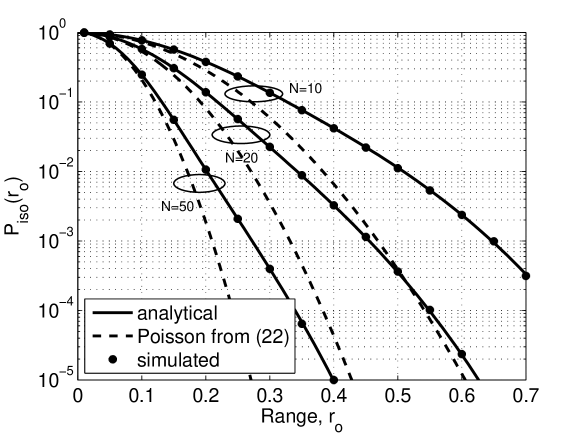
Fig. 16 plots the probability of node isolation, Piso(ro)subscript𝑃isosubscript𝑟oP_{\textrm{iso}}(r_{\textrm{o}}), in (19), versus thetransmission range rosubscript𝑟or_{\textrm{o}} for N=10,20,50𝑁102050N=10,20,50 nodes. The probability of node isolation in infinite homogenous Poisson point process networks [12]

Piso(ro)subscript𝑃isosubscript𝑟o\displaystyle P_{\textrm{iso}}(r_{\textrm{o}}) =eρπro2,absentsuperscript𝑒𝜌𝜋superscriptsubscript𝑟o2\displaystyle=e^{-\rho\pi r_{\textrm{o}}^{2}}, (22)

assuming constant node density ρ=10,20,50𝜌102050\rho=10,20,50 nodes/m2 is also plotted as a reference. We can see from Fig. 16 that the simulation results for finite networks match perfectly with the numerical results. This is to be expected since we account for boundary effects accurately and evaluate (19) exactly. Fig. 16 shows that the probability of node isolation is greater in finite networks, compared with Poisson networks. This is due to the inclusion of the border and corner effects, as explained in Section III.
Refer to caption
Figure 16: Probability of node isolation, Piso(ro)subscript𝑃isosubscript𝑟oP_{\textrm{iso}}(r_{\textrm{o}}), versus the transmission range rosubscript𝑟or_{\textrm{o}} for N=10,20,50𝑁102050N=10,20,50 nodes independently and uniformly distributed in a unit square.

V-B Minimum Node Degree Distribution and k𝑘k-Connectivity

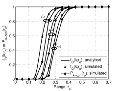
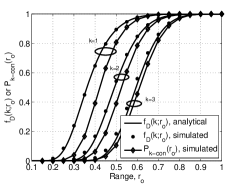
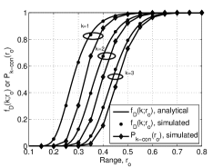
Here, through simulations, we validate our framework to determine the minimum node degree distribution. Using (III-B), we determine the minimum node degree distribution fD(k;ro)subscript𝑓𝐷𝑘subscript𝑟of_{D}(k;r_{\textrm{o}}) for k=1,2,3𝑘123k=1,2,3 and for number of nodes N=10,20,50𝑁102050N=10,20,50. The simulation results for fD(k;ro)subscript𝑓𝐷𝑘subscript𝑟of_{D}(k;r_{\textrm{o}}) are obtained by uniformly distributing the N𝑁N nodes in a square region, each with transmission range rosubscript𝑟or_{\textrm{o}}, over a square region and determining if the minimum of number of neighbors for all nodes in the network are equal to k𝑘k. Note that the simulation results for fD(k;ro)subscript𝑓𝐷𝑘subscript𝑟of_{D}(k;r_{\textrm{o}}) are obtained by averaging over all S=50,000𝑆50000S=50,000 random topologies for each rosubscript𝑟or_{\textrm{o}} and k𝑘k . The simulation results for fD(k;ro)subscript𝑓𝐷𝑘subscript𝑟of_{D}(k;r_{\textrm{o}}) are also plotted in Fig. 17 and match perfectly with the analytical results using (III-B).

As highlighted earlier in Section II-B, the probability of k𝑘k-connectivity Pk-con(ro)subscript𝑃k-consubscript𝑟oP_{\textrm{k-con}}(r_{\textrm{o}}) is bounded by the minimum node degree distribution fD(k;ro)subscript𝑓𝐷𝑘subscript𝑟of_{D}(k;r_{\textrm{o}}). This is because we obtain a k𝑘k-connected network at the same time when we obtain a network with minimum node degree k𝑘k, both with and without boundary effects [15, 12, 14]. Here we validate through simulation results that the minimum node degree distribution fD(k;ro)subscript𝑓𝐷𝑘subscript𝑟of_{D}(k;r_{\textrm{o}}) serves as an upper bound for Pk-con(ro)subscript𝑃k-consubscript𝑟oP_{\textrm{k-con}}(r_{\textrm{o}}) and the bound gets tighter as Pk-con(ro)subscript𝑃k-consubscript𝑟oP_{\textrm{k-con}}(r_{\textrm{o}}) approaches one.

We repeat the simulation environment of Section V-B and now for each of the 50,0005000050,000 random topologies, we measure the k𝑘k-connectivity of the network for k=1,2,3𝑘123k=1,2,3. The simulation results for Pk-con(ro)subscript𝑃k-consubscript𝑟oP_{\textrm{k-con}}(r_{\textrm{o}}) are plotted in Fig. 17 along with the analytical results for minimum node degree distribution fD(k;ro)subscript𝑓𝐷𝑘subscript𝑟of_{D}(k;r_{\textrm{o}}) obtained using (III-B) and our proposed framework. It is evident in the plots that the relation between fD(k;ro)subscript𝑓𝐷𝑘subscript𝑟of_{D}(k;r_{\textrm{o}}) and Pk-con(ro)subscript𝑃k-consubscript𝑟oP_{\textrm{k-con}}(r_{\textrm{o}}) given in (6) holds, that is, fD(k;ro)Pk-con(ro)subscript𝑓𝐷𝑘subscript𝑟osubscript𝑃k-consubscript𝑟of_{D}(k;r_{\textrm{o}})\rightarrow P_{\textrm{k-con}}(r_{\textrm{o}}) as Pk-con(ro)1subscript𝑃k-consubscript𝑟o1P_{\textrm{k-con}}(r_{\textrm{o}})\rightarrow 1.

We note that the simulation tests for k𝑘k-connectivity are computationally intensive and the computational complexity to check k𝑘k-connectivity scales with Nk1superscript𝑁𝑘1N^{k-1} for k2𝑘2k\geq 2. For example, the complexity to check 111-connectivity and 222-connectivity is of the order O(N+S)𝑂𝑁𝑆O(N+S) and the complexity to determine 333-connectivity is O(N(N+S))𝑂𝑁𝑁𝑆O(N(N+S)), where S𝑆S denotes the number of simulations. However, (III-B) can be evaluated numerically very easily. This illustrates an advantage of the proposed framework over simulations.
Refer to caption
(a) N=10𝑁10N=10
Refer to caption
(b) N=20𝑁20N=20
Refer to caption
(c) N=50𝑁50N=50
Figure 17: Minimum node degree distribution, fD(k;ro)subscript𝑓𝐷𝑘subscript𝑟of_{D}(k;r_{\textrm{o}}) and probability of k𝑘k-connectivity, P1-con(ro)subscript𝑃1-consubscript𝑟oP_{\textrm{1-con}}(r_{\textrm{o}}), versus transmission range rosubscript𝑟or_{\textrm{o}} for (a) N=10𝑁10N=10, (b) N=20𝑁20N=20 and (c) N=50𝑁50N=50 nodes independently and uniformly distributed in a unit square.

V-C 111-Connectivity

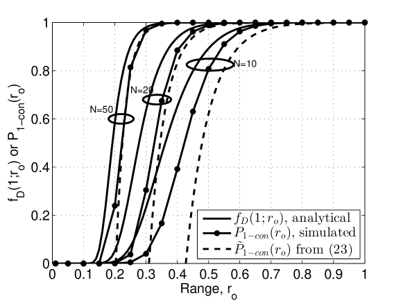
Since P1-con(ro)subscript𝑃1-consubscript𝑟oP_{\textrm{1-con}}(r_{\textrm{o}}) is one of the essential characteristics of wireless multi-hop networks, we analyze the tightness of the bound provided by fD(1;ro)subscript𝑓𝐷1subscript𝑟of_{D}(1;r_{\textrm{o}}) for P1-con(ro)subscript𝑃1-consubscript𝑟oP_{\textrm{1-con}}(r_{\textrm{o}}) in more detail and compare with the existing bounds in the literature.

Fig. 18 plots the fD(1;ro)subscript𝑓𝐷1subscript𝑟of_{D}(1;r_{\textrm{o}}) as an upper bound for the probability of connectivity (obtained via simulations), versus transmission range rosubscript𝑟or_{\textrm{o}} for N=10,20,50𝑁102050N=10,20,50 nodes. For comparison, we plot the high density approximation for P1-con(ro)subscript𝑃1-consubscript𝑟oP_{\textrm{1-con}}(r_{\textrm{o}}) which is derived in [27] using a cluster expansion approach as

P~1-con(ro)subscript~𝑃1-consubscript𝑟o\displaystyle\tilde{P}_{\textrm{1-con}}(r_{\textrm{o}}) 1L2ρeπβρ4Lβπeπ2βρ16βρπeπ4βρ,absent1superscript𝐿2𝜌superscript𝑒𝜋𝛽𝜌4𝐿𝛽𝜋superscript𝑒𝜋2𝛽𝜌16𝛽𝜌𝜋superscript𝑒𝜋4𝛽𝜌\displaystyle\approx 1-L^{2}\rho e^{-\frac{\pi}{\beta}\rho}-4L\sqrt{\frac{\beta}{\pi}}e^{-\frac{\pi}{2\beta}\rho}-\frac{16\beta}{\rho\pi}e^{-\frac{\pi}{4\beta}\rho}, (23)

where L𝐿L denotes the side length, ρ𝜌\rho denotes the node density and β=(ro/L)2𝛽superscriptsubscript𝑟o𝐿2\beta=(r_{\textrm{o}}/L)^{-2}.

Refer to caption
Figure 18: Probability of connectivity: Upper bound as minimum node degree distribution, fD(k;ro)subscript𝑓𝐷𝑘subscript𝑟of_{D}(k;r_{\textrm{o}}), high density approximation P~1-con(ro)subscript~𝑃1-consubscript𝑟o\tilde{P}_{\textrm{1-con}}(r_{\textrm{o}}) and simulated P1-con(ro)subscript𝑃1-consubscript𝑟oP_{\textrm{1-con}}(r_{\textrm{o}}), versus transmission range rosubscript𝑟or_{\textrm{o}} for N=10,20,50𝑁102050N=10,20,50 nodes independently and uniformly distributed in a unit square.

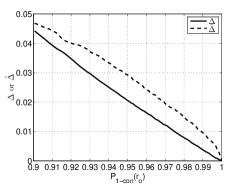
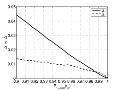
The high density approximation in (23) is comparatively a better estimate for P1-con(ro)subscript𝑃1-consubscript𝑟oP_{\textrm{1-con}}(r_{\textrm{o}}) for N=50𝑁50N=50 nodes but is not useful for N=10𝑁10N=10 nodes. We analyze the tightness of the bounds in more detail over the value of probabilities in the interval 0.9P1-con(ro)10.9subscript𝑃1-consubscript𝑟o10.9\leq P_{\textrm{1-con}}(r_{\textrm{o}})\leq 1. The differences between the bounds, Δ=|P1-con(ro)fD(1;ro)|Δsubscript𝑃1-consubscript𝑟osubscript𝑓𝐷1subscript𝑟o\Delta=|{P_{\textrm{1-con}}(r_{\textrm{o}})}-f_{D}(1;r_{\textrm{o}})| and Δ~=|P1-con(ro)P~1-con(ro)|~Δsubscript𝑃1-consubscript𝑟osubscript~𝑃1-consubscript𝑟o\tilde{\Delta}=|{P_{\textrm{1-con}}(r_{\textrm{o}})}-\tilde{P}_{\textrm{1-con}}(r_{\textrm{o}})| is plotted in Fig. 19 for 0.9P1-con(ro)10.9subscript𝑃1-consubscript𝑟o10.9\leq P_{\textrm{1-con}}(r_{\textrm{o}})\leq 1. For small number of nodes (N=10,20𝑁1020N=10,20), it can be noted that the proposed minimum node degree distribution fD(1;ro)subscript𝑓𝐷1subscript𝑟of_{D}(1;r_{\textrm{o}}) is comparatively a tight bound for P1-con(ro)subscript𝑃1-consubscript𝑟oP_{\textrm{1-con}}(r_{\textrm{o}}) than the high density approximation P~1-con(ro)subscript~𝑃1-consubscript𝑟o\tilde{P}_{\textrm{1-con}}(r_{\textrm{o}}).

On the basis of simulation results presented here and in the previous section, we can say that the upper bound for the connectivity provided by the minimum node degree distribution in (6) provides a good approximation for the simulation results when P1-con(ro)1subscript𝑃1-consubscript𝑟o1P_{\textrm{1-con}}(r_{\textrm{o}})\approx 1. This is consistent with the observation in [14] for circular areas with or without boundary effects. Thus, the proposed framework can be used to accurately predict the network connectivity properties even when the number of nodes is small.

V-D Network Design Example: Minimum Transmission Range and Minimum Number of Nodes

We now address the network design problems: a) Determine the minimum transmission range r0csuperscriptsubscript𝑟0𝑐r_{0}^{c} for given number of nodes or b) Find are the minimum number of nodes Ncsuperscript𝑁𝑐N^{c}, each with given transmission range rosubscript𝑟or_{\textrm{o}}, such that the network is k𝑘k-connected with high probability Pk-con(ro)subscript𝑃k-consubscript𝑟oP_{\textrm{k-con}}(r_{\textrm{o}}), say 0.95 or 0.99. Such a minimum value transmission range and the minimum number of nodes to achieve the desired level of Pk-con(ro)subscript𝑃k-consubscript𝑟oP_{\textrm{k-con}}(r_{\textrm{o}}) are often termed as critical transmission range and critical number of nodes respectively [12, 31, 9]. For a given transmission range, the minimum number of nodes must be deployed to minimize the cost and reduce the interference between the nodes [12]. For a network with fixed number of nodes, the transmission range must be large enough to ensure the network connectivity but it should be small enough to minimize the power consumption and reduce the interference between the nodes.
Refer to caption
(a) N=10𝑁10N=10
Refer to caption
(b) N=20𝑁20N=20
Refer to caption
(c) N=50𝑁50N=50
Figure 19: The differences Δ=|P1-con(ro)fD(1;ro)|Δsubscript𝑃1-consubscript𝑟osubscript𝑓𝐷1subscript𝑟o\Delta=|{P_{\textrm{1-con}}(r_{\textrm{o}})}-f_{D}(1;r_{\textrm{o}})| and Δ~=|P1-con(ro)P~1-con(ro)|~Δsubscript𝑃1-consubscript𝑟osubscript~𝑃1-consubscript𝑟o\tilde{\Delta}=|{P_{\textrm{1-con}}(r_{\textrm{o}})}-\tilde{P}_{\textrm{1-con}}(r_{\textrm{o}})| denotes the deviation of simulated P1-con(ro)subscript𝑃1-consubscript𝑟oP_{\textrm{1-con}}(r_{\textrm{o}}) from the proposed bound as minimum node degree distribution fD(1;ro)subscript𝑓𝐷1subscript𝑟of_{D}(1;r_{\textrm{o}}) in (III-B) and high density approximation P~1-con(ro)subscript~𝑃1-consubscript𝑟o\tilde{P}_{\textrm{1-con}}(r_{\textrm{o}}) given in (23) respectively. Both ΔΔ\Delta and Δ~~Δ\tilde{\Delta} are plotted for (a) N=10𝑁10N=10, (b) N=20𝑁20N=20 and (c) N=50𝑁50N=50.

Since Pk-con(ro)subscript𝑃k-consubscript𝑟oP_{\textrm{k-con}}(r_{\textrm{o}}) is a monotonic function of both transmission range rosubscript𝑟or_{\textrm{o}} and the number of nodes N𝑁N, the solution to the above problem is to determine the curve in N𝑁N-rosubscript𝑟or_{\textrm{o}} plane for which Pk-con(ro)=0.95subscript𝑃k-consubscript𝑟o0.95P_{\textrm{k-con}}(r_{\textrm{o}})=0.95 or Pk-con(ro)=0.99subscript𝑃k-consubscript𝑟o0.99P_{\textrm{k-con}}(r_{\textrm{o}})=0.99. We can carry out simulations to determine rocsuperscriptsubscript𝑟o𝑐r_{\textrm{o}}^{c} or Ncsuperscript𝑁𝑐N^{c}. However, as highlighted earlier, it would be very computationally intensive to obtain simulation results with sufficient accuracy, especially for large values of k𝑘k. We demonstrate here that we can obtain analytical solutions to the design problems mentioned above using the proposed framework. Recalling that minimum node degree distribution fD(k;ro)subscript𝑓𝐷𝑘subscript𝑟of_{D}(k;r_{\textrm{o}}) serves as a good approximation for Pk-con(ro)subscript𝑃k-consubscript𝑟oP_{\textrm{k-con}}(r_{\textrm{o}}), we can use fD(k;ro)subscript𝑓𝐷𝑘subscript𝑟of_{D}(k;r_{\textrm{o}}) given in (III-B) to determine the critical transmission range and critical number of nodes. The surface plot for fD(1;ro)subscript𝑓𝐷1subscript𝑟of_{D}(1;r_{\textrm{o}}) is shown in Fig. 20 as a function of the number of nodes N𝑁N and the transmission range rosubscript𝑟or_{\textrm{o}}, where we have also shown the analytical curves consisting of (N,ro)𝑁subscript𝑟o(N,r_{\textrm{o}}) pairs for which fD(1;ro)=0.95subscript𝑓𝐷1subscript𝑟o0.95f_{D}(1;r_{\textrm{o}})=0.95 or fD(1;ro)=0.99subscript𝑓𝐷1subscript𝑟o0.99f_{D}(1;r_{\textrm{o}})=0.99 and the simulation curves denoting (Nc,roc)superscript𝑁𝑐superscriptsubscript𝑟o𝑐(N^{c},r_{\textrm{o}}^{c}) pairs for which P1-con(ro)=0.95subscript𝑃1-consubscript𝑟o0.95P_{\textrm{1-con}}(r_{\textrm{o}})=0.95 or P1-con(ro)=0.99subscript𝑃1-consubscript𝑟o0.99P_{\textrm{1-con}}(r_{\textrm{o}})=0.99 with the tolerance of ±0.5%plus-or-minuspercent0.5\pm 0.5\%. It can be observed that the analytical determination of (Nc,roc)superscript𝑁𝑐superscriptsubscript𝑟o𝑐(N^{c},r_{\textrm{o}}^{c}) using the proposed minimum node degree distribution fD(1;ro)subscript𝑓𝐷1subscript𝑟of_{D}(1;r_{\textrm{o}}) yields a fairly good approximation for both P1-con(ro)=0.95subscript𝑃1-consubscript𝑟o0.95P_{\textrm{1-con}}(r_{\textrm{o}})=0.95 and P1-con(ro)=0.99subscript𝑃1-consubscript𝑟o0.99P_{\textrm{1-con}}(r_{\textrm{o}})=0.99. Nevertheless, by virtue of our analysis in the previous section and Penrose theorem on connectivity of random graphs [15], the analytical determination is more accurate for P1-con(ro)=0.99subscript𝑃1-consubscript𝑟o0.99P_{\textrm{1-con}}(r_{\textrm{o}})=0.99.

Refer to caption
Figure 20: Surface plot for fD(1;ro)subscript𝑓𝐷1subscript𝑟of_{D}(1;r_{\textrm{o}}) as a function of number of nodes N𝑁N and transmission range rosubscript𝑟or_{\textrm{o}}. The curves denote (N,ro)𝑁subscript𝑟o(N,r_{\textrm{o}}) pairs for which fD(1;ro)=0.95,subscript𝑓𝐷1subscript𝑟o0.95f_{D}(1;r_{\textrm{o}})=0.95, or 0.990.990.99 and (Nc,roc)superscript𝑁𝑐superscriptsubscript𝑟o𝑐(N^{c},r_{\textrm{o}}^{c}) pairs for which Pk-con(ro)=0.95±0.5%subscript𝑃k-consubscript𝑟oplus-or-minus0.95percent0.5P_{\textrm{k-con}}(r_{\textrm{o}})=0.95\pm 0.5\% or 0.99±0.5%plus-or-minus0.99percent0.50.99\pm 0.5\%.

VI Conclusions

In this paper, we have presented a tractable analytical framework for the exact calculation of the probability of node isolation and the minimum node degree distribution in finite wireless sensor networks. We have considered N𝑁N sensor nodes, each with transmission range rosubscript𝑟or_{\textrm{o}}, which are independently and uniformly distributed in a square region. The proposed framework can accurately account for the boundary effects by partitioning the square into subregions, based on the transmission range and the node location. The exact modeling of the boundary effects has not been taken into consideration in previous studies in the literature. Our results confirm that the boundary effects play a key role in determining the connectivity metrics of the network: probability of node isolation, minimum node degree distribution and probability of k𝑘k-connectivity, especially when the number of nodes is small (N<50(N<50). We have also validated the proposed framework with the help of simulations.

Future research can consider natural generalizations of the work presented here. Firstly, the proposed framework can be extended for the case of polygon region (generalization of square region). Secondly, the consideration of the channel fading and interference in the transmission model (generalization of disk model) is an open problem which is outside the scope of this work.

Appendix A Minimum Node Degree Distribution

Here, we present the formulation of the probability distribution of the minimum node degree D𝐷D presented in (3). For N𝑁N uniformly distributed nodes, the number of neighbors d𝑑d for a node located at 𝒖𝒖\boldsymbol{u} follows a binomial distribution [12, 14, 24]

(N1d)(F(𝒖;ro))d(1F(𝒖;ro))Nd1binomial𝑁1𝑑superscript𝐹𝒖subscript𝑟o𝑑superscript1𝐹𝒖subscript𝑟o𝑁𝑑1\binom{N-1}{d}\left(F(\boldsymbol{u};r_{\textrm{o}})\right)^{d}\left(1-F(\boldsymbol{u};r_{\textrm{o}})\right)^{N-d-1}

and the probability that any node in the network has at least d𝑑d neighbors is therefore given by

(N1d)(F(𝒖;ro))d(1F(𝒖;ro))Nd1𝑑s(𝒖).binomial𝑁1𝑑subscriptsuperscript𝐹𝒖subscript𝑟o𝑑superscript1𝐹𝒖subscript𝑟o𝑁𝑑1differential-d𝑠𝒖\binom{N-1}{d}\int_{\mathcal{R}}\left(F(\boldsymbol{u};r_{\textrm{o}})\right)^{d}\left(1-F(\boldsymbol{u};r_{\textrm{o}})\right)^{N-d-1}ds(\boldsymbol{u}).

Now the probability that any node in the network has at least k𝑘k neighbors can be expressed as

1d=0k1(N1d)(F(𝒖;ro))d(1F(𝒖;ro))Nd1𝑑s(𝒖),1superscriptsubscript𝑑0𝑘1binomial𝑁1𝑑subscriptsuperscript𝐹𝒖subscript𝑟o𝑑superscript1𝐹𝒖subscript𝑟o𝑁𝑑1differential-d𝑠𝒖1-\sum_{d=0}^{k-1}\binom{N-1}{d}\int_{\mathcal{R}}\left(F(\boldsymbol{u};r_{\textrm{o}})\right)^{d}\left(1-F(\boldsymbol{u};r_{\textrm{o}})\right)^{N-d-1}ds(\boldsymbol{u}),

which gives rise to the minimum node degree distribution fD(k;ro)=P(D=k)subscript𝑓𝐷𝑘subscript𝑟oP𝐷𝑘f_{D}(k;r_{\textrm{o}})=\textrm{P}(D=k) that all the nodes have at least k𝑘k neighbors, with an assumption of independence between the nodes. This leads to the result in (3).

References

  • [1] P. Gupta and P. R. Kumar, “Internet in the sky: The capacity of three dimensional wireless networks,” Comm. in Information and Systems, vol. 1, pp. 33–49, 2001.
  • [2] X. Hong, M. Gerla, H. Wang, and L. Clare, “Load balanced, energy-aware communications for mars sensor networks,” in Proc. IEEE Aerospace Conference, vol. 3, 2002.
  • [3] D. Puccinelli and M. Haenggi, “Wireless sensor networks: applications and challenges of ubiquitous sensing,” IEEE Circuits and Systems Magazine, vol. 5, no. 3, pp. 19–31, 2005.
  • [4] J.-H. Cui, J. Kong, M. Gerla, and S. Zhou, “The challenges of building mobile underwater wireless networks for aquatic applications,” IEEE Network, vol. 20, no. 3, pp. 12–18, May-June 2006.
  • [5] F. Li and Y. Wang, “Routing in vehicular ad hoc networks: A survey,” IEEE Vehicular Technology Magazine, vol. 2, no. 2, pp. 12–22, 2007.
  • [6] P. Fan, G. Li, K. Cai, and K. Letaief, “On the geometrical characteristic of wireless ad-hoc networks and its application in network performance analysis,” IEEE Trans. Wireless Commun., vol. 6, no. 4, pp. 1256–1265, Apr. 2007.
  • [7] F. Fabbri, C. Buratti, and R. Verdone, “A multi-sink multi-hop wireless sensor network over a square region: Connectivity and energy consumption issues,” in Proc. IEEE GLOBECOM, 2008, pp. 1–6.
  • [8] J. G. Andrews, R. K. Ganti, M. Haenggi, N. Jindal, and S. Weber, “A primer on spatial modeling and analysis in wireless networks,” IEEE Commun. Mag., vol. 48, no. 11, pp. 156–163, Nov. 2010.
  • [9] P.-J. Wan, C.-W. Yi, and L. Wang, “Asymptotic critical transmission radius for k𝑘k-connectivity in wireless ad hoc networks,” IEEE Trans. Inf. Theory, vol. 56, no. 6, pp. 2867–2874, 2010.
  • [10] G. Mao, “Research on wireless multi-hop networks: Current state and challenges,” in Proc. ICCNC, 2012.
  • [11] F. Baccelli and B. Blaszczyszyn, Stochastic geometry and wireless networks, volume 1 & 2: Theory and applications.   Foundations and Trends in Networking, 2009.
  • [12] C. Bettstetter, “On the minimum node degree and connectivity of a wireless multihop network,” Proc. 3rd ACM International Symposium on Mobile Ad Hoc Networking & Computing, vol. 9, no. 11, pp. 80–91, 2002.
  • [13] Z. Khalid and S. Durrani, “Connectivity of three dimensional wireless sensor networks using geometrical probability,” in Proc. Australian Communications Theory Workshop (AusCTW), 2013, pp. 47–51.
  • [14] C. Bettstetter, “On the connectivity of ad hoc networks,” The Computer Journal, vol. 47, no. 4, pp. 432–447, 2004.
  • [15] M. Penrose, “The longest edge of the random minimal spanning tree,” The Annals of Applied Probability, vol. 7, no. 2, pp. 340–361, 1997.
  • [16] P. Gupta and P. Kumar, “Critical power for asymptotic connectivity in wireless networks,” in Proc. IEEE CDC, vol. 1, 1998, pp. 1106–1110.
  • [17] Q. Ling and Z. Tian, “Minimum node degree and k-connectivity of a wireless multihop network in bounded area,” in Proc. IEEE GLOBECOM, 2007, pp. 1296–1301.
  • [18] D. Miorandi, E. Altman, and G. Alfano, “The impact of channel randomness on coverage and connectivity of ad hoc and sensor networks,” IEEE Trans. Wireless Commun., vol. 7, no. 3, pp. 1062–1072, Mar. 2008.
  • [19] X. Zhou, H. Jones, S. Durrani, and A. Scott, “Effect of beamforming on the connectivity of ad hoc networks,” in Proc. Australian Communications Theory Workshop (AusCTW), 2007, pp. 13–18.
  • [20] X. Zhou, S. Durrani, and H. M. Jones, “Connectivity analysis of wireless ad hoc networks with beamforming,” IEEE Trans. Veh. Technol., vol. 58, no. 9, pp. 5247–5257, Nov. 2009.
  • [21] S. C. Ng, G. Mao, and B. D. O. Anderson, “Critical density for connectivity in 2D and 3D wireless multi-hop networks,” IEEE Trans. Wireless Commun., vol. 12, no. 4, pp. 1512–1523, 2013.
  • [22] W. Jia and J. Wang, “Analysis of connectivity for sensor networks using geometrical probability,” IEE Proceedings Communications, vol. 153, no. 2, pp. 305–312, Apr. 2006.
  • [23] F. Fabbri and R. Verdone, “A statistical model for the connectivity of nodes in a multi-sink wireless sensor network over a bounded region,” in Proc. 14th European Wireless Conference, June 2008.
  • [24] S. Srinivasa and M. Haenggi, “Distance distributions in finite uniformly random networks: Theory and applications,” IEEE Trans. Veh. Technol., vol. 59, no. 2, pp. 940–949, Feb. 2010.
  • [25] A. Eslami, M. Nekoui, H. Pishro-Nik, and F. Fekri, “Results on finite wireless sensor networks: Connectivity and coverage,” ACM Trans. Sen. Netw., vol. 9, no. 4, pp. 51:1–51:22, Jul. 2013.
  • [26] G. Mao and B. D. O. Anderson, “Towards a better understanding of large-scale network models,” IEEE/ACM Transactions on Networking, vol. 20, no. 2, pp. 408–421, Apr. 2012.
  • [27] J. P. Coon, C. P. Dettmann, and O. Georgiou, “Full connectivity: Corners, edges and faces,” J. Stat. Phys., vol. 147, pp. 758–778, 2012.
  • [28] A. M. Mathai, An introduction to geometrical probability: Distributional aspects with applications.   CRC Press, 1999.
  • [29] G.-C. Aboue Nze, F. Guinand, and Y. Pigne, “Impact of square environment on the connectivity in finite ad hoc networks,” in Proc. 14th International Symposium on Wireless Personal Multimedia Communications (WPMC), 2011.
  • [30] R. Rajagopalan and P. Varshney, “Connectivity analysis of wireless sensor networks with regular topologies in the presence of channel fading,” IEEE Trans. Wireless Commun., vol. 8, no. 7, pp. 3475–3483, Jul. 2009.
  • [31] P.-J. Wan and C.-W. Yi, “Asymptotic critical transmission ranges for connectivity in wireless ad hoc networks with bernoulli nodes,” in Proc. IEEE Wireless Communications and Networking Conference, 2005, vol. 4, 2005, pp. 2219–2224.
  • [32] P. Santi, D. M. Blough, and F. Vainstein, “A probabilistic analysis for the range assignment problem in ad hoc networks,” in Proc. 2nd ACM international symposium on Mobile ad hoc networking &\& computing.   New York, NY, USA: ACM, 2001, pp. 212–220.
  • [33] Z. Khalid and S. Durrani, “Distance distributions in regular polygons,” IEEE Trans. Veh. Technol., vol. 62, no. 5, pp. 2363–2368, Jun. 2013.
  • [34] U. Bäsel, “Random chords and point distances in regular polygons,” ArXiv Technical Report, 2012. [Online]. Available: http://arxiv.org/abs/1204.2707
  • [35] M. K. Simon and M.-S. Alouini, Digital Communication over fading channels, 2nd ed.   Wiley, 2005.
  • [36] G.-C. Nze and F. Guinand, “Mean degree of ad hoc networks in environments with obstacles,” in Proc. IEEE 8th International Conference on Wireless and Mobile Computing, Networking and Communications (WiMob), 2012, pp. 381–388.