Invariants of Montesinos Twins

Abstract.

In [Gil82], C. Giller proposed an invariant of ribbon $2$-knots in $S^{4}$ based on a type of skein relation for a projection to $\mathbb{R}^{3}$. In certain cases, this invariant is equal to the Alexander polynomial for the $2$-knot. Giller’s invariant is, however, a symmetric polynomial — which the Alexander polynomial of a $2$-knot need not be. After modifying a $2$-knot into a Montesinos twin in a natural way, we show that Giller’s invariant is related to the Seiberg-Witten invariant of the exterior of the twin, glued to the complement of a fiber in $E(2)$.

1. Introduction

A smooth $2$-knot $K$ in the $4$-sphere is an embedded $S^{2}$ in $S^{4}$ considered up to smooth isotopy. We say that $K$ is unknotted when it bounds a smoothly embedded $D^{3}\subset S^{4}$. In contrast to classical knot theory, $2$-knots display many pathologies; their exteriors need not be a $K(\pi_{1},1)$ [AC59] nor does the homeomorphism type of the knot complement determine the knot’s isotopy class [Gor76]. After a surgery which replaces the regular neighborhood $\nu K\cong S^{2}\times D^{2}$ with $D^{3}\times S^{1}$ we obtain a homology $S^{1}\times S^{3}$. With $b_{2}^{+}=b_{2}=0$ for such a manifold, current tools for smooth $4$-manifolds offer few invariants.

However, the natural generalizations of gadgets like the Alexander polynomial or ideal can be computed for $2$-knots. In [Gil82], C. Giller proposed a definition for an invariant we will call $\Delta_{G}$. The proposed invariant is derived from a kind of skein relation on the projection to $\mathbb{R}^{3}$ of a $2$-knot analogous to the Conway skein relation for projections of $1$-knots to $\mathbb{R}^{2}$. For a certain class of $2$-knots, $\Delta_{G}$ is known to compute the Alexander polynomial. This relation, which we discuss more thoroughly in section 1.8, always results in a symmetric polynomial. However, the Alexander polynomial of a $2$-knot need not be symmetrizable. For example, the knot shown in Figure 7 has Alexander polynomial $\Delta_{A}=1-2t$ while Giller’s polynomial is $\Delta_{G}=t^{-2}-1+t^{2}$. Further complicating matters is that Giller’s polynomial was not actually known to be an invariant.

If instead of $2$-knots, we look at “twins” in $S^{4}$, we have objects to which gauge-theoretic methods can be applied. It is in this context we see that Giller’s polynomial computes, in the relevant cases, the Seiberg-Witten invariant of the exterior of the twin.

1.1. Twins

In [Mon83] and [Mon84], J. M. Montesinos introduced the concept of a twin in $S^{4}$. Such an object consists of a pair of $2$-knots $K_{1},K_{2}$ which meet transversely twice. As the second homology of $S^{4}$ is trivial, these intersection points must come with opposite signs. By “standard twins”, we will mean that both $K_{i}$ are unknotted and that the exterior of the pair is diffeomorphic to $T^{2}\times D^{2}$. We construct these explicitly below. In general, the exterior of a twin is a homology $T^{2}\times D^{2}$ with boundary diffeomorphic to $T^{3}$.

As $\pi_{2}(SO(2))$ is trivial, an orientation on an $2$-knot $K$ in $S^{4}$ determines a trivialization $\nu S^{2}\cong S^{2}\times D^{2}$. That is, for a $2$-knot $K$, all framings are equivalent to the Seifert framing. Fix orientations on the $2$-knots, $K_{1},K_{2}$, in a twin ${\mathbb{T}\mathrm{w}}$ and consider $\partial\nu{\mathbb{T}\mathrm{w}}\cong T^{3}$. Take a simple closed curve $\gamma$ on the twin passing through the intersection points of $K_{1},K_{2}$ and lift it to $\partial\nu{\mathbb{T}\mathrm{w}}$ using the framings. All such $\gamma$ are isotopic on the twin and, as each $K_{i}$ has a single framing, this lift is canonical. This decomposes $\partial\nu{\mathbb{T}\mathrm{w}}=\gamma\times T^{2}$ The boundaries of normal discs $D^{2}_{1},D^{2}_{2}$ to $K_{1},K_{2}$ refine the decomposition to $\partial\nu{\mathbb{T}\mathrm{w}}=\gamma\times\partial D^{2}_{1}\times\partial D^{2}_{2}$.

With this decomposition in mind, we define a standard surgery for a twin ${\mathbb{T}\mathrm{w}}$ in $S^{4}$. Let

$$S^{4}_{{\mathbb{T}\mathrm{w}}}=(S^{4}\setminus{\mathbb{T}\mathrm{w}})\operatorname*{\cup}_{\phi}(T^{2}\times D^{2})$$

where $\phi:T^{3}\to T^{3}$ identifies the $\partial D^{2}$ from $T^{2}\times D^{2}$ with $\gamma$. Up to isotopy, any two such $\phi$ differ by a diffeomorphism $T^{2}\times\text{pt}\to T^{2}\times\text{pt}$. Since any such map extends over $T^{2}\times D^{2}$, the resulting manifold only depends on the embedding of the twin. Also, $H_{*}(S^{4}_{{\mathbb{T}\mathrm{w}}};\mathbb{Z})\cong H_{*}(T^{2}\times S^{2};\mathbb{Z})$ so that the $2$-torus core, $T_{{\mathbb{T}\mathrm{w}}}$, of the surgery is identified with $T^{2}\times pt\subset T^{2}\times S^{2}$ as a homology class.

1.2. Definition of the invariant for twins

Let $F$ be a smooth fiber in an elliptic fibration of $E(2)$, the underlying smooth manifold for a complex $K3$ surface. The regular neighborhood of the fiber, $\nu F$, comes with a trivialization $\nu F=D^{2}\times T^{2}$ induced by the fibration giving us the identification $\partial\nu F=\partial D^{2}\times F$. Taking a twin ${\mathbb{T}\mathrm{w}}\subset S^{4}$, we also have a decomposition $\partial{N}({\mathbb{T}\mathrm{w}})=\gamma\times\partial D^{2}_{1}\times\partial D^{2}_{2}$. If we fix an identification of this $\partial D^{2}_{1}\times\partial D^{2}_{2}$ and $F$ and an orientation reversing diffeomorphism between $\partial D^{2}$ and $\gamma$, we obtain an identification $\phi$ of $\partial(E(2)\setminus\nu F)$ and $\partial(S^{4}\setminus{\mathbb{T}\mathrm{w}})$. Let

$$E(2)_{{\mathbb{T}\mathrm{w}}}=(E(2)\setminus\nu F)\operatorname*{\cup}_{\phi}(S^{4}\setminus{\mathbb{T}\mathrm{w}}).$$

Since any automorphism of $F$ exends smoothly over $E(2)\setminus\nu F$, this construction depends on the smooth isotopy class of $F$ but is independant, up to diffeomorphism, of the particular choice of $\phi$. As $\pi_{1}(E(2)\setminus\nu F)=0$ and the image of $\pi_{1}(T^{3})$ normally generates $\pi_{1}(S^{4}\setminus{\mathbb{T}\mathrm{w}})$, $E(2)_{{\mathbb{T}\mathrm{w}}}$ is simply connected. Then an easy Meyer-Vietoris argument shows that $E(2)$ and $E(2)_{{\mathbb{T}\mathrm{w}}}$ have the same cohomology ring. By Freedman’s theorem, $E(2)$ and $E(2)_{{\mathbb{T}\mathrm{w}}}$ are homeomorphic.

This procedure may also be thought of as the generalized fiber sum of $E(2)$ and $S^{4}_{{\mathbb{T}\mathrm{w}}}$ along $F$ and the core $T_{{\mathbb{T}\mathrm{w}}}$ of the surgered twin with its default framing. As such, we will sometimes write $E(2)_{{\mathbb{T}\mathrm{w}}}$ as $E(2)\operatorname*{\#}_{F=T_{{\mathbb{T}\mathrm{w}}}}S^{4}_{{\mathbb{T}\mathrm{w}}}$.

The invariant of the twin ${\mathbb{T}\mathrm{w}}$ which we will consider will be the Seiberg-Witten invariant of $E(2)_{{\mathbb{T}\mathrm{w}}}$. i.e.

Definition 1.2.1.

$I({\mathbb{T}\mathrm{w}})=SW(E(2)_{{\mathbb{T}\mathrm{w}}})$ thought of as an element of the group ring $\mathbb{Z}\left[H_{2}(E(2))\right]$.

Precisely, $SW(E(2)_{{\mathbb{T}\mathrm{w}}})$ lives in $\mathbb{Z}\left[H_{2}(E(2)_{{\mathbb{T}\mathrm{w}}})\right]$ which we identify with $H_{2}(E(2))$ by a homomorphism which extends the identity map on $H_{2}(E(2)_{{\mathbb{T}\mathrm{w}}}\setminus(S^{4}\setminus\nu{\mathbb{T}\mathrm{w}}))\to H_{2}(E(2)\setminus\nu F)$. The invariant is well defined up to a sign which depends on a homology orientation of $H_{0}(E(2))\oplus\det H_{2}^{+}(E(2))\oplus H_{1}(E(2))$

As the standard twins ${\mathbb{T}\mathrm{w}}_{std}$ have complement diffeomorphic to $T^{2}\times D^{2}$, $E(2)_{{\mathbb{T}\mathrm{w}}_{std}}$ is diffeomorphic to $E(2)$ and

(1) $$I({\mathbb{T}\mathrm{w}}_{std})=SW(E(2))=1.$$

Now suppose that we have a twin ${\mathbb{T}\mathrm{w}}$ and a disjoint torus $T$ in $S^{4}$. As $T$ is null-homologous, it has a canonical framing given by the outward normal of its Seifert manifold. We can then form the self fiber sum $S^{4}_{{\mathbb{T}\mathrm{w}}}\operatorname*{\#}_{T_{\mathbb{T}\mathrm{w}}=T}$. With a choice of an identification of $T_{\mathbb{T}\mathrm{w}}$ and $T$, the result is well defined and any choice of identification will have the same Seiberg-Witten polynomial, due to the gluing formulas of [MMS97]. Then form

$$E(2)_{{\mathbb{T}\mathrm{w}},T}=E(2)\operatorname*{\#}_{F=T_{{\mathbb{T}\mathrm{w}}}^{\prime}}\left(S^{4}_{{\mathbb{T}\mathrm{w}}}\operatorname*{\#}_{T_{\mathbb{T}\mathrm{w}}=T}\right)$$

with $T_{{\mathbb{T}\mathrm{w}}}^{\prime}$ a pushoff of $T_{{\mathbb{T}\mathrm{w}}}$. Our new manifold $E(2)_{{\mathbb{T}\mathrm{w}},T}$ is a homology $E(2)\operatorname*{\#}_{F=F^{\prime}}$ with $F,F^{\prime}$ elliptic fibers and $SW(E(2)\operatorname*{\#}_{F=F^{\prime}})=(t-t^{-1})^{2}$ with $t=\exp([F])$. See [MMS97]. We define

Definition 1.2.2.

$I({\mathbb{T}\mathrm{w}},T)=(t-t^{-1})^{-1}SW(E(2)_{{\mathbb{T}\mathrm{w}},T})$ thought of as a element of the group ring $\mathbb{Z}\left[H_{2}(E(2);\mathbb{Z})\right]$.

1.3. Construction of Knotted twins

Construction 1.3.1 (Connect sum).

Take $K_{0}$, a knotted $S^{2}$, and a twin ${\mathbb{T}\mathrm{w}}=K_{1}\operatorname*{\cup}K_{2}$ in $S^{4}$. Then, selecting one of the spheres $K_{1}$ in the twin, we form the connected sum $(S^{4}\operatorname*{\#}S^{4},K_{0}\operatorname*{\#}K_{1})$ at some point away from the 2 double points of the twins. (This construction is not independent of the choice of $K_{1},K_{2}$ in ${\mathbb{T}\mathrm{w}}$ in general.)

If we take ${\mathbb{T}\mathrm{w}}$ to be the standard twins, then this construction is independent of the choice of $S^{2}$s and provides a handy method for studying $2$-knots via twins. This independence is due to the existence of a orientation preserving diffeomorphism $\rho$ of $S^{4}$ which interchanges $K_{1},K_{2}$ in standard twins. The diffeomorphism $\rho$ is constructed as follows: View $S^{4}$ as $\nu{\mathbb{T}\mathrm{w}}_{std}\operatorname*{\cup}T^{2}\times D^{2}$. Define $\rho$ on $\nu{\mathbb{T}\mathrm{w}}_{std}$ to be the obvious map which interchanges $K_{1}$ and $K_{2}$. Then $\rho$ induces the map

$$\left[\begin{array}[]{ccc}0&1&0\\ 1&0&0\\ 0&0&1\end{array}\right]$$

on $\partial\nu{\mathbb{T}\mathrm{w}}_{std}=T^{2}\times\partial D^{2}=T^{3}$ under the basis for $H_{1}(T^{3})$ given by $\partial D^{2}_{K_{1}},\partial D^{2}_{K_{2}},$ and $\partial D^{2}_{T^{2}}$ where $\partial D^{2}_{S}$ is the boundary of the normal bundle to $S$. This map then extends over $T^{2}\times D^{2}$ giving $\rho$ on $S^{3}$.

Construction 1.3.2 (Artin Spin).

This construction is originally due to E. Artin in [Art26]. To each smooth knot $K$ in $S^{3}$ and let $\widehat{K}$ be the corresponding arc in $D^{3}$ obtained by removing a small $D^{3}$ surrounding a point of $K$. We can arrange $\widehat{K}$ so that it meets $\partial D^{3}$ perpendicularly at the north and south poles. Clearly $S^{3}\setminus\nu K$ and $D^{3}\setminus\nu\widehat{K}$ are diffeomorphic.

Using the decomposition $S^{4}=D^{2}\times S^{2}\cup S^{1}\times D^{3}$, we can identify the $4$-sphere with the space $(S^{1}\times D^{3})/\sim$ where $(\theta_{0},x_{0})\sim(\theta_{1},x_{1})$ iff $x_{0}=x_{1}\in\partial D^{3}$.

Let $K_{1},K_{2}$ be, respectively, the images of $\{1\}\times\partial D^{3}$ and the $S^{1}\times\dot{K}$ under $\sim$. Each is a smoothly embedded $2$-sphere which intersect each other pairwise at the images of the north and south poles of $\partial D^{3}$. Thus $K_{1}$ and $K_{2}$ form twins ${\mathbb{T}\mathrm{w}}_{K}$. The first sphere, $K_{1}$, bounds $\{1\}\times D^{3}$ in $S^{4}$ and if $\Sigma$ is a Seifert surface for $K$, then $K_{2}$ bounds $S^{1}\times\Sigma$ union a $2$-handle attached along $S^{1}\times\text{pt}$. The loop $\gamma$, connecting the intersection points of the $K_{i}$, bounds a copy $\Sigma$ in the complement of the twin.

In fact, $S^{4}\setminus\nu{\mathbb{T}\mathrm{w}}_{K}$ is diffeomorphic to $S^{1}\times(S^{3}\setminus\nu K)$. In the case that $K$ is the unknot, we get the standard twins $S^{4}\setminus\nu{\mathbb{T}\mathrm{w}}_{K}=S^{1}\times(S^{1}\times D^{2})=T^{2}\times D^{2}$. See Figure 1.

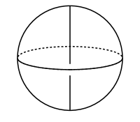
Figure 1. Spin to get standard twins

When the standard twin surgery is performed on twins formed by Artin spinning $K$, the result is the manifold $S^{1}\times S^{3}_{0}(K)$. (Where $S^{3}_{0}(K)$ is the result of zero surgery on $K\subset S^{3}$.) This case is identical to the knot surgery considered by Fintushel and Stern in [FS98] and so we have

Theorem 1.3.3 (Fintushel, Stern).

$I({\mathbb{T}\mathrm{w}}_{K})=\Delta_{K}(t^{2})$ where $\Delta_{K}$ is the symmetrized Alexander polynomial of $K$ and $t=\exp([F])$.

Construction 1.3.4 (Twist Spin).

As before, given a knot $K$ in $S^{3}$ we obtain a knotted arc $\widehat{K}$ in $D^{3}$ with boundary on the north and south poles. For each $\theta\in S^{1}=\mathbb{R}/2\pi\mathbb{Z}$ let $\widehat{K}_{n\theta}$ be the image of $\widehat{K}$ rotated by $n\theta$ radians about the $z$-axis. The annulus $A_{n}$ in $S^{1}\times D^{3}$ is obtained by taking the union of $\{\theta\}\times\widehat{K}_{n\theta}$. This annulus descends to a knotted $S^{2}$, $K_{2}$, in $S^{4}=S^{1}\times B^{3}/\sim$.

Together with $K_{1}$, the image of $\{\theta\}\times\partial B^{3}$, we form a twin. We call $K_{2}$ the $n$-twist spin of $K$ and write $K_{2}=\tau^{n}K$ and ${\mathbb{T}\mathrm{w}}_{\tau^{n}K}$ for the associated twin.

As with the Artin spin, the first sphere, $K_{1}$, bounds $\{1\}\times D^{3}$ in $S^{4}$. The loop $\gamma$, connecting the intersection points of the $K_{i}$, bounds a copy $\Sigma$ in the complement of the twin.

This construction is due to Zeeman, who in [Zee65], showed that the $n$-twist spin of a knot was not isotopic to any $2$-knot obtained by Artin spinning when $n>1$. The $n=1$ case is interesting in that the $1$-twist spin, $\tau K$ is unknotted independently of choice of $K$. However, the twin ${\mathbb{T}\mathrm{w}}_{\tau K}$ is typically knotted. This provides an interesting example of twins in which both $2$-knots are unknots but with the twins being knotted as an interchangable pair. See [GK78].

Construction 1.3.5 (Roll Spin).

Similar to the twist spin, this construction involves a deformation of a knotted arc $\widehat{K}$ in $D^{3}$ fixing the north and south poles which returns the arc to the starting point. Take a international date line of $\partial D^{3}$ union $\widehat{K}$ and push it into $D^{3}\setminus\widehat{K}$ so that it is null homologous. Call this $\widehat{K}$. Then consider the $1$-parameter family of diffeomorphisms given by pushing a base point $x$ $n$ times along $\widehat{K}$. The return map $\phi$ is then a diffeomorphism of the quadruple $(D^{3},\partial D^{3},\widehat{K},x)$ which is the identity on all but the first component. Since $\phi$ is isotopic to the identity rel $\partial D^{3}$, $S^{1}\times D^{3}$ is diffeomorphic to $\mathbb{R}\times D^{3}/(+1,\phi)$. Let the annulus $A$ be the image of $\mathbb{R}\times\widehat{K}/(+1,\phi)$ in $S^{1}\times D^{3}$.

Then, as before, $A$ becomes a $2$-knot $K_{2}$ in $S^{4}$ after quotienting by $\sim$. We call $K_{2}$ the $n$-roll spin of $K$ and write $K_{2}=\rho^{n}K$ and ${\mathbb{T}\mathrm{w}}_{\rho^{n}K}$ for the associated twin.

The roll spinning construction is due to Fox who, in [Fox66], showed that, for $\widehat{K}=\widehat{4_{1}}$, the knotted $2$-sphere $K_{2}$ coming from the deformed arc is not isotopic to any $n$-twist spun knot. In this case, the $1$-roll spin had a corresponding visualization, duplicated in Figure 2, of the motion of $\widehat{K_{1}}$ in $D^{3}$ which explains why the word “roll” was chosen to describe this construction.

Figure 2. Fox’s Roll Spin

Note that both twist and roll spinning can be described in terms of certain diffeomorphisms of $D^{3}$ which keep $\partial D^{3}$ and $\widehat{K}$ fixed identically. With this in mind, we now consider their mutual generalization, Deform spinning:

Construction 1.3.6 (Deform Spin).

Let $\phi$ be a self diffeomorphism of $D^{3}$ keeping $\partial D^{3},\widehat{K}$ and a base point $p$ fixed identically. Then the mapping torus of $\phi$ is $S^{1}\times D^{3}\cong(\mathbb{R}\times D^{3})/\left<(r,x)\sim(r+1,\phi(x))\right>$ with an embedded annulus $\widehat{K_{2}}$ which is the quotient of $\mathbb{R}\times\widehat{K}$. Then after quotienting by the identification $(\theta_{0},x)\sim(\theta_{1},x)$ for $x\in\partial D^{3}$ as before, we obtain a knotted $2$-sphere $K_{2}$, the image of $\widehat{K_{2}}$, which together with $K_{1}$, the image of $\{\theta\}\times\partial D^{3}$, forms a twin. We write $K_{2}=\phi K$ and ${\mathbb{T}\mathrm{w}}_{\phi K}$ for the twin pair. The isotopy class of $K_{2}$ and of ${\mathbb{T}\mathrm{w}}_{\phi K}$ is determined solely by the isotopy class of $\phi$.

This construction was introduced by Litherland in [Lit79]. Diffeomorphisms such as $\phi$ are called “deformations” and form a group $\mathcal{D}(K)$ of deformations modulo isotopy. $\mathcal{D}(K)$ is isomorphic to the group $\operatorname{Aut}_{\partial}(\pi_{1}(S^{3}\setminus K))$ of automorphisms of $\pi_{1}(S^{3}\setminus K)$ preserving the fixed peripheral subgroup given by the image $\pi_{1}(\partial\nu K)\to\pi_{1}(S^{3}\setminus\nu K)$. In this setup we find that $\tau$ corresponds to conjugation by the meridian of $K_{1}$ and $\rho$ corresponds to conjugation by the longitude of $K_{1}$. Then

Lemma 1.3.7 (Litherland).

If $K_{1}$

• is not a torus knot, $\mathbb{Z}_{\tau}\oplus\mathbb{Z}_{\rho}\subset\mathcal{D}(K_{1})$.

• is a $p,q$-torus knot, $\tau^{pq}\rho=\operatorname{id}$ and $\mathcal{D}(K_{1})\cong\mathbb{Z}_{\tau}$.

In the case that $K$ is a composite knot, $K=\#_{i\in I}K_{i}$, the deformation group $D(K)$ may be much larger than the subgroup generated by $\rho,\tau$ and includes a copy of the pure braid group on $|I|$ strands; see [Gra77].

1.4. Ribbon Knots and Twins

We say that a 2-knot $K$ is ribbon if it is formed by the following construction: Let $D=\operatorname*{\sqcup}D^{3}$ (bases), $B=\operatorname*{\sqcup}D^{2}\times I$ (bands) each be embedded in $\mathbb{R}^{4}$ with $(\partial D)\cap B=\operatorname*{\sqcup}D^{2}\times\pm 1$. If a band intersects a base elsewhere,

$$\left(D^{2}\times(-1,1)\right)\cap D^{3}=D^{2}\times t,\quad t\in(-1,1)$$

and

$$\left(D^{2}\times(-1,1)\right)\cap(\partial D^{3})=\emptyset.$$

The second type of intersection is called a ribbon intersection of $K$ or ribbon singularity of $D\operatorname*{\cup}B$. Then

$$K=(\partial D\setminus\underbrace{\operatorname*{\sqcup}D^{2}\times\pm 1}_{\text{in }\partial B})\operatorname*{\cup}(\operatorname*{\sqcup}(\partial D^{2})\times I)$$

is a ribbon knot with ribbon presentation given by $D\operatorname*{\cup}B$. We can define ribbon surfaces of arbitrary genus in the same manner.

Suppose that we have a twin ${\mathbb{T}\mathrm{w}}=K_{1}\operatorname*{\cup}K_{2}$ for which the $K_{i}$ are ribbon. Then for each $K_{i}$ we have a set of bases $D_{i}$ and bands $B_{i}$. We will say that ${\mathbb{T}\mathrm{w}}$ is ribbon if

1. $B_{1}\cap B_{2}=\emptyset$

2. $D_{1}\cap B_{2}=\operatorname*{\sqcup}D^{2}\times t$, $t\in(-1,1)$ with $(\partial D_{1})\cap D^{2}\times(-1,1)=\emptyset$ for each band in $B_{2}$ (ribbon intersection)

3. $D_{2}\cap B_{1}=\operatorname*{\sqcup}D^{2}\times t$, $t\in(-1,1)$ with $(\partial D_{2})\cap D^{2}\times(-1,1)=\emptyset$ for each band in $B_{1}$ (ribbon intersection)

4. $D_{1}\cap D_{2}=2D^{2}$. More specifically, $D_{1}$ and $D_{2}$ meet only in two balls $D^{\prime}_{i},D^{\prime\prime}_{i}$ from each and at these intersections (corresponding to the intersection points $K_{1}\cap K_{2}$), we have the following local model:

   $$D^{\prime}_{1}=\left\{(z_{1},z_{2})\in\mathbb{C}^{2}\mid\text{Re}(z_{2})\leq 1,\text{Im}(z_{2})=0\right\}\subset\mathbb{C}^{2},$$

   $$D^{\prime}_{2}=\left\{(z_{1},z_{2})\in\mathbb{C}^{2}\mid\text{Re}(z_{1})\leq 1,\text{Im}(z_{1})=0\right\}\subset\mathbb{C}^{2},$$

   So that taking the boundary of each gives us the cone of the positive Hopf link. The $D^{\prime\prime}_{1},D^{\prime\prime}_{2}$ case is the same but with orientations reversed on $D^{\prime\prime}_{2}$, giving us a negative Hopf link cone boundary.

In this case we say that ${\mathbb{T}\mathrm{w}}$ is a ribbon twin.

It is known that of the deform spun knots, only the Artin and 1-twist spun knots are ribbon. Hence, at most Artin and 1-twist spun twins may be ribbon. Artin spun twins are known to be ribbon but it is not known to the author if 1-twist spun twins are ribbon.

Two ribbon presentations are stably equivalent if they are equivalent under the following operations. Addition of a trivial base/band pair, sliding the disc to which a band attaches (band slide), and moving a ribbon intersection along a base/band sequence (band pass) are shown in Figure 3 and together with isotopy generate stable equivalence of ribbon presentations. Clearly stable equivalence of ribbon presentations generates isotopies of the corresponding ribbon knot but the converse also holds — isotopic ribbon knots have stably equivalent ribbon presentations. For a proof of this, see [Mar92].

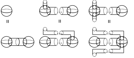
Figure 3. A) Trivial addition/deletion B) Band slide C) Band pass

It will occasionally be easier to deal with simplified ribbon presentations. Let $\Gamma=\Gamma(D,B)$ be the graph which has vertices corresponding to bases and edges given by bands, connected in the natural way. It is clear that $b_{1}(\Gamma)$ is the genus of the ribbon surface specified by the ribbon presentation. We restrict ourselves to the case where the ribbon surface is a sphere or torus. Suppose that $\Gamma$ has a vertex $x$ of valence $3$ or greater. Then one of the outgoing edges of $x$ has a path which ends at a vertex $y$ with a single incoming edge. Perform the band slide corresponding to this path to get a new ribbon presentation $\Gamma^{\prime}$ with the same set of bases. In $\Gamma^{\prime}$, the valence of $x$ has decreased by $1$ and the valence of $y$ is now $2$. Continue this procedure until we arrive at a graph $\widehat{\Gamma}$ (and corresponding ribbon presentation) for which each vertex has valence at most $2$. Then, as cell complexes, $\widehat{\Gamma}$ is either an interval or a circle as the ribbon surface is a sphere or a torus. We will call such ribbon presentations linear.

Consider the connect sum of a ribbon $2$-knot $K_{0}$ with standard twins ${\mathbb{T}\mathrm{w}}=K_{1}\operatorname*{\cup}K_{2}$. Standard twins have a simple ribbon presentation given by two bases and a band each. (Each base is for one of the twin intersection points.) Stabilize the band in $K_{1}$ by switching it for two bands and a base. Then the connect sum $K_{0}\operatorname*{\#}K_{1}$ is formed by adding a band from the new base of $K_{0}$ to any of the terminal bases in a ribbon presentation of $K_{1}$.

1.5. Projections

In the study of knots in $\mathbb{R}^{3}$, a generic projections to $\mathbb{R}^{2}$, together with crossing information, completely determines the isotopy type of a knot. Similarly, there is a theory for decorated projections for twins and surfaces in $\mathbb{R}^{4}=S^{4}\setminus\text{pt}$ which determines their embedding up to isotopy.

Giller proves, in [Gil82], that if $\Sigma$ is a surface in $\mathbb{R}^{4}$, then up to isotopy $\Sigma$ admits a projection to $\mathbb{R}^{3}$ with only double and triple points exist. Further, such projections are generic. In these generic projections, the double points either exist in families which are either simple closed curves or embedded open intervals whose closed endpoints are triple points. See Figure 4. In the same paper, he gives methods of decorating these projections with over – middle – under crossing information and a way of determining if an arbitrary set of crossing information gives a lift of such an immersion of a surface in $\mathbb{R}^{3}$ to an embedding in $\mathbb{R}^{4}$.

Figure 4. Local models for a family of double points and a triple point

We will only consider those knots and twins which admit a projection which contain no triple points. Not all twins or surfaces have such a projection and those that do are said to be simply knotted. First examples of simply knotted $2$-knots include Artin spun knots and ribbon $2$-knots. For Artin spun knots, we can get a projection with no triple points by doing the same spinning construction (one dimension down) to the projection to $\mathbb{R}^{2}$ of the original, classical knot. This creates an $S^{1}$s worth of double points for each crossing in the classical knot’s projection. We will call a twin ${\mathbb{T}\mathrm{w}}=K_{1}\operatorname*{\cup}K_{2}$ simply knotted if both $K_{i}$ are simply knotted and pairwise have no triple points.

Ribbon knots have embedded projections away from the ribbon singularities — the intersections of the interiors of bands with interiors of the bases. (This is in contrast with ribbon $1$-knots, for which projections of non-intersecting bands may have crossings. The analogous situation for $2$-knots is an under/over crossing of the whole band — which does not result in a crossing in the projection to $\mathbb{R}^{3}$.) Nearby the ribbon singularities, we have projections which appear as in Figure 5. It was proved in [Yaj64] that all simply knotted $S^{2}$s are ribbon.

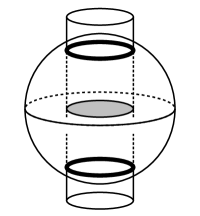
Figure 5. A projection of the neighborhood of a ribbon singularity (shaded disc) and the corresponding two $S^{1}$s of double points.

When we have a $S^{1}$ family of double points, we have local neighborhoods around each which appear as in the first picture in Figure 4. This gives the neighborhood of the family the structure of an bundle over $S^{1}$. As the surfaces in $\mathbb{R}^{4}$ are orientable and the two preimages of the double points are separated, the monodromy must be trivial. This means that, local to the $S^{1}$ family of double points, the projection is that of a classical knot crossing times $S^{1}$.

Then, for a simply knotted projection of a (oriented) surface in $\mathbb{R}^{4}$, it is sufficient to label one of the surfaces as being over crossing at each family of double points. We will use “+” to denote this.

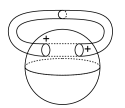
Figure 6. A sphere and a torus with crossing information.

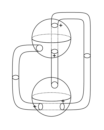
Figure 7. A $2$-knot with Alexander polynomial $1-2t$ and Giller polynomial $\Delta_{G}=t^{-2}-1+t^{2}$

For a twin, a few additional pieces of information are needed. We need to keep track of the two intersection points of the spheres. In $S^{4}$, the neighborhood of each is diffeomorphic to the cone on a positive or negative Hopf link. Then the (undecorated) projection of such a neighborhood appears as does a neighborhood of double points. We decorate the projection with a solid dot to indicate the intersection point of the $S^{2}$s and $+$ signs to indicate over/under crossings on the double point arcs which emanate from it. We switch from over to under at the intersection of the spheres in twins. See Figure 8

Figure 8. The projection of the neighborhood of the intersection of spheres in a twin. To the left, the vertical plane crosses above and to the right, the horizontal does.

1.6. Virtual knot presentation

In [Sat00], Satoh showed how to represent ribbon surfaces of genus $0$ and $1$ in $\mathbb{R}^{4}$ by means of virtual knots/links. For our purposes, a virtual knot (or link) is a diagram in $\mathbb{R}^{2}$ of embedded, oriented arcs which end either at “crossings” as in the (top) first two pictures in Figure 9 or at endpoints as in the (top) third picture. Each such diagram corresponds to a collection of immersed surfaces in $\mathbb{R}^{3}$ by replacing each of the crossings and endpoints in Figure 9 with the corresponding surfaces in $\mathbb{R}^{3}$ shown. These are then connected via tubes parallel to the embedded arcs. Thus, any virtual link corresponds to the projection, with crossing information, of a collection of ribbon $2$-spheres and tori in $\mathbb{R}^{4}$.

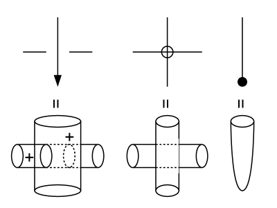
Figure 9. Correspondence of crossings in virtual knots to crossings in projections of surfaces to $\mathbb{R}^{3}$

Conversely, linear ribbon presentations of knots correspond to virtual knots. Take a projection of $K\subset\mathbb{R}^{4}\to\mathbb{R}^{3}$ having only double points at ribbon singularities. For each band in the linear ribbon presentation, consider the image of its core in $\mathbb{R}^{3}$ extended to the center of the bases to which the band attaches. This gives an immersed (at ribbon singularities) arc $\widehat{K}$ in $\mathbb{R}^{3}$. Taking a generic projection $\mathbb{R}^{3}\to\mathbb{R}^{2}$ we get an arc $\widecheck{K}$ immersed in $\mathbb{R}^{2}$ with two kinds of singularities:

• double points of the projection $\widehat{K}\subset\mathbb{R}^{3}\to\mathbb{R}^{2}\supset\widecheck{K}$ and

• projections of immersion points $\widehat{K}\hookrightarrow\mathbb{R}^{3}$.

Each of the first kind of double point corresponds to a virtual crossing. For the second kind of crossing we must first consider a diversion about orientations.

The endpoints of $\widecheck{K}$ each correspond to a base with only one band attached — here, $K$ locally consists of the discs $D_{1},D_{2}$. With a fixed orientation on $K$, we orient the boundary of the $D_{i}$ with the outward normal. We then say that the endpoint of $\widecheck{K}$ is out/in as the boundary orientation on the $D_{i}$ is counterclockwise or clockwise, respectively (when $D_{i}$ is orientation-preserving identified with the unit complex disc.) This orients $\widecheck{K}$.

Then, with $\widecheck{K}$ oriented, we can check that the second type of immersion point corresponds to the ribbon intersection in Figure 9. If it does not (i.e. the two crossings have the opposite under/over information) then perform the isotopy in Figure 10. Once this has been done, we may use our correspondence from Figure 9 to label each of the immersion points of $\widecheck{K}$ as virtual knot crossings.

Figure 10. Fixing a “bad” ribbon crossing by an isotopy which creates two virtual crossings

In addition to the “classical” Reidemeister moves in Figure 11, associated to a virtual knot, we have the series of “virtual” Reidemeister moves in Figure 12 giving allowable isotopies. Notice that move D is one of the forbidden moves of the virtual knots of Kauffman. The type of virtual knot we consider here is sometimes referred to a being weakly virtual but in the spirit of brevity we will omit “weakly” in this paper. These concepts of virtual knots are inequivalent as there are virtual knots, in the sense of Kauffman, which are knotted and which, when move D is allowed, are unknotted. Such an example is given in [Sat00].

Figure 11. Reidemeister Moves for Classical knots

Figure 12. “Reidemeister” Moves for Virtual knots

We will add additonal markings to describe ribbon twins. For a ribbon twin ${\mathbb{T}\mathrm{w}}=K_{1}\operatorname*{\cup}K_{2}$, there are two bases $D^{\prime}_{i},D^{\prime\prime}_{i}$ in the ribbon representation of each $K_{i}$ which correspond to the twin intersection points $K_{1}\cap K_{2}$. Perform band slides until the ribbon presentations of the $K_{i}$ are linear with endpoints $D^{\prime}_{i},D^{\prime\prime}_{i}$. Then we have corresponding virtual knot representations of the $K_{i}$ with identical endpoints. We will use $\oplus,\ominus$ to mark each of these as they correspond to the cone on the positive and negative Hopf bands at the intersection points. With this in mind, we get the moves in Figure 13.

Figure 13. “Reidemeister” Moves $F1$,$F2$ for Twins, versions for $\ominus$ are identical

Now let us consider the connect sum of a ribbon $2$-knot $K_{0}$ with standard twins ${\mathbb{T}\mathrm{w}}=K_{1}\operatorname*{\cup}K_{2}$ as described in Section 1.4. Recall that, in this construction, we formed the connect sum by adding a single band between bases of $K_{1}$ and $K_{0}$. We can assume that $K_{1}$ has a ribbon presentation with $3$ bases, $D_{+},D_{0},D_{-}$ with the positive/negative twin intersections occuring at $D_{+}$ and $D_{-}$ respectively. This ribbon presentation has $2$ bands, $B_{+}$ from $D_{+}$ to $D_{0}$ and $B_{-}$ from $D_{0}$ to $D_{-}$. Assume that $K_{0}$ is given by a virtual knot diagram and hence that it has a linear ribbon decomposition. Let $B_{0}$ be a band connecting the base $D_{0}$ on $K_{1}$ and endpoints of the linear ribbon decomposition of $K_{0}$. Then $K_{1}\#K_{0}$ has a ribbon decomposition in the shape of a $T$, with the top bar cosisting of the bands $B_{\pm}$ and the shaft consiting of $B_{0}$ and the ribbon decomposition for $K_{0}$.

To get a virtual knot diagram for the twin ${\mathbb{T}\mathrm{w}}\#K_{0}$, we will need to perform a series of band slides – sliding one of $B_{\pm}$ along the ribbon decomposition of $K_{0}$ to the other endpoint. This is straightforward and results in a ribbon decomposition whose virtual knot diagram can be obtained from that of $K_{0}$ by

1. replace each strand of the virtual knot for $K_{0}$ with two parallel strands,

2. at the two endpoints of the virtual knot, replace the endpoint with one of diagrams show in the bottom of the first two columns of Figure 14, using both,

3. replace crossings for the virtual knot for $K_{0}$ with configurations as shown in Figure 14.

An example is shown in Figure 15.

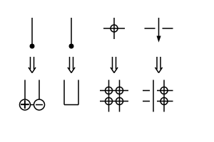
Figure 14. Ribbon knot to connect sum ribbon twin

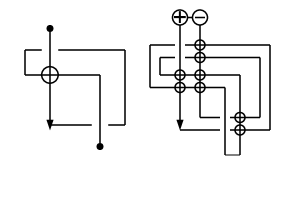
Figure 15. Giller’s example (left) and its connect sum with standard twins (right)

Another technique for obtaining a Ribbon twin from a ribbon $2$-knot $K_{1}$ is to take a virtual knot presentation for $K_{1}$ and perform virtual Reidemesiter moves so that the endpoint-bases sit in the unbounded region of the plane. Then connect these using an crossingless arc sitting in the unbounded face. This gives the second, unknotted, $2$-sphere $K_{2}$ of the twin. For example, see Figure 16

Figure 16. Giller’s example (left) and twin containing it (right)

1.7. Surgery diagrams

As discussed earlier, a twin in $S^{4}$ has a canonical surgery associated to it. Since our decorated projections determine isotopy type, no additional information is needed to carry out surgery. For a $T^{2}$ in $S^{4}$, however, we will need additional information.

As any $T^{2}\subset S^{4}$ is nullhomologous, it bounds a Seifert manifold which, via its inward normal, gives a Seifert framing for the $T^{2}$. This gives us a decomposition, $\partial\nu T^{2}=T^{2}\times S^{1}$. As surgery replacing $\nu T^{2}$ with $T^{2}\times D^{2}$ is determined by the image of $\partial D^{2}$, we see that we can entirely describe surgery by specifying a curve on $T^{2}$ and an integer giving the winding about a meridian (boundary of normal disc) to $T^{2}$. See Figure 17.

When the $T^{2}$ is ribbon with a linear ribbon presentation and corresponding virtual knot diagram, we can decompose $T^{2}$ in the following manner: Let $C$ be the core of the ribbon presentation, projected to $\mathbb{R}^{3}$. Let $\alpha$ be an essential loop on $T^{2}$ which, when projected to $\mathbb{R}^{3}$ is null-homologous in $\mathbb{R}^{3}\setminus C$. Any such loop represents the same homology class on $T^{2}$. Let $\beta$ be $\partial D^{2}\times\{t\}$ in a band in the ribbon presentation. Orient $\alpha$ to coincide with the orientation of the virtual knot diagram. Then orient $\beta$ so that $\alpha\cdot\beta=+1$ with respect to the orientation on $T^{2}$. So $T^{2}\cong\alpha\times\beta$. Then, in the virtual knot diagram, labeling the knot corresponding to $T^{2}$ with $(\gamma,\beta/\alpha)$ where $\gamma$ is the winding number of the attached $\partial D^{2}$ with respect to the Seifert framing and $\beta/\alpha$ is the slope of $\partial D^{2}$ projected to $T^{2}$.

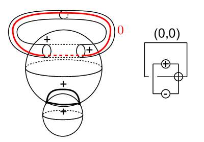
Figure 17. Projection and Virtual Knot surgery diagrams for a twin and torus.

We will write an $S$ together with $*$s on the appropriate components when we wish to denote this surgery.

1.8. Giller’s Polynomial

In [Gil82], C. Giller defines a polynomial $\Delta_{G}(t)$ of simply knotted $S^{2}$s in $S^{4}$. This supposed invariant obeys a skein relation similar to that of the Alexander polynomial for classical knots.

That is, consider a embedded circle of double points in a projection of a (collection of) oriented sphere or torus in $\mathbb{R}^{4}$. As mentioned before, we can trivialize the neighborhood of the double points so that we have the neighborhood of a classical knot crossing times $S^{1}$. All surfaces in question are oriented and so orient the double points of their projection — this orients both strands in the classical picture. We can then replace this neighborhood with $S^{1}$ times any of the $3$ options in Figure 18, obtaining

Figure 18. Resolution of a knot crossing

The invariant is then defined by the relation:

(2) $$\Delta_{G}(L_{+})-\Delta_{G}(L_{-})=(t^{1/2}-t^{-1/2})\Delta_{G}(L_{0})$$

together with

(3) $$\Delta_{G}(\text{unknotted sphere})=1$$

and

(4) $$\Delta_{G}(\text{surfaces separated by an }S^{3})=0.$$

Giller also describes $\Delta_{G}$ in a manner similar to that of the Alexander polynomial. That is, letting $M$ be a Seifert manifold for $K$, he forms the infinte cyclic cover $X$ of $S^{4}\setminus K$ and presents $H_{1}(X)$ as a $\mathbb{Q}[t,t^{-1}]$ module. Then $\Delta_{G}$ is defined by $T=\mathbb{Q}[t,t^{-1}]/(\Delta_{G})$ where $T$ is the $\mathbb{Q}[t,t^{-1}]$ torsion part of $H_{1}(X)$.

Whenever $K$ is ribbon, we can choose $M$ to be a punctured $nS^{1}\times S^{2}$ given by the ribbon presentation. It is easy to verify by standard arguments that isotopies and band-stabilizations of the ribbon presentation yeild the same $\Delta_{G}$. Therefore, $\Delta_{G}$ is well-defined for ribbon knots.

For Artin spun knots, Giller’s polynomial is the Alexander polynomial. In the case that we apply these computations to the projection of the knotted sphere in an Artin spun twin, Giller’s polynomial is the Seiberg-Witten polynomial. (as shown in [FS98]).

Interestingly, $2$-knots and twins need not have a symmetric Alexander polynomial. Giller’s polynomial and the Seiberg-Witten polynomial, however, are symmetric. For example, see Figure 7, which is the spun right hand trefoil with crossing changes.

The natural questions to ask are then: Is Giller’s polynomial an invariant of $2$-knots? If so, is it equal to the Seiberg-Witten polynomial for the corresponding twin? For twins, what is the relationship between the Alexander polynomial and the Seiberg-Witten invariant? Our invariant provides suggestive evidence that the second question, at least in some cases, should be answered in the affirmative.

2. The $4$-dimensional Conway moves

2.1. $3$-dimensional Hoste Move

The main theorem of Fintushel and Stern in [FS98] gives a way of computing the Seiberg-Witten Invariants of classical-knot surgered $4$-manifolds in terms of the symmetrized Alexander polynomial of the knot. The proof relies on a technique J. Hoste developed in [Hos84] which is a method for obtaining Kirby calculus diagrams for so called “sewn-up $r$-link exteriors” in $S^{3}$. (Like Fintushel and Stern, we will only consider the case where $r$-links are actually knots and links.) We discuss a simplified but sufficient version of the original move below so to demonstrate the ideas involved.

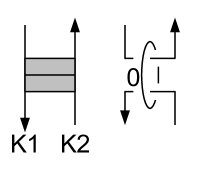
Figure 19. $3$-dimensional Hoste move

A sewn up knot exterior is formed by taking either two oriented knots in one copy of $S^{3}$ or in two separate copies, excising a normal neighborhood of each knot, and gluing the resulting boundary $T^{2}$s by a diffeomorphism. For our purposes, we will let the diffeomorphism be the one which identifies oriented meridians and longitudes for the Seifert framings of each knot.

This procedure does two things, it removes two copies of $S^{1}\times D^{2}$ with a chosen framing and orientation, and it replaces them with an $S^{1}\times S^{1}\times I$. Together, these are the boundary of $S^{1}\times D^{2}\times I$. Thus we may think of forming a sewn up link exterior as the result (on the boundary) of adding a round $4$-dimensional $1$-handle to $B^{4}$ so that the feet of the round $1$-handle are the two knots, each with the proper framing.

Now, consider a projection of a link $L$ in $S^{3}$ with oriented components $K_{1}$, $K_{2}$ and a small region in the projection where $K_{1}$ and $K_{2}$ run parallel but in opposite directions. We can then connect $K_{1}$ and $K_{2}$ via an arc. See Figure 19. Attach the round handle as above to form the sewn up link exterior for $K_{1}$ and $K_{2}$. Note that we can choose the attaching map of the round handle so that in the corresponding Morse-Bott function, the points $p_{1},p_{2}$ on $K_{1},K_{2}$ where the arc touches each knot are both connected to the same point $p$ on the critical $S^{1}$ by gradient flow lines.

Take a perfect Morse function on the critical $S^{1}$ of the round handle so that the index zero critical point is $p$. This decomposes the round $1$-handle into a $1$-handle and $2$-handle corresponding to the $0$- and $1$-handles of the Morse function on $S^{1}$.

Figure 20. Round handle becomes a $1$ and $2$ handle

Attaching the $1$-handle to $S^{3}$ results in self connect summing $S^{3}$ at the points $p_{1},p_{2}$. By standard tricks, this is the same as zero surgery on the unknot around the arc in the second drawing in Figure 19.

The attaching circle of the $2$-handle is the “band sum” $K$ of $K_{1}$ and $K_{2}$ as shown in Figure 20 and the second picture in Figure 19. Attaching the $2$-handle to the result (an $S^{1}\times S^{2}$) of the previous surgery is then merely zero surgery on $K$.

2.2. $4$-dimensional Hoste Move

In [FS98], the Hoste move shows up in $4$-dimensions with an $S^{1}$ equivariance as we cross the $3$-manifold with $S^{1}$. When that is done, the surgeries on knots show up as surgeries on square zero tori which, by using [MMS97], are amenable to computations of the Seiberg-Witten invariant. The $4$-dimensional version of the Hoste move we will discuss here does not assume this $S^{1}$ equivariance, although local $S^{1}$ equivariances will occur.

Proposition 2.2.1.

Consider two embedded, oriented square zero tori $T_{1},T_{2}$ in a $4$-manifold $X$. Suppose that $T_{1},T_{2}$ are connected by an annulus $A=S^{1}\times I$, embedded in $X$, so that $\partial A$ consists of an essential curve on each torus. Let each $T_{i}$ be framed so that $A\cap\partial\nu T_{i}$ is in the subspace of $H_{1}(\partial\nu T_{i})=H_{1}(T^{3})$ generated by the pushoffs of loops on $T_{i}$ with respect to the framing. Let $\phi$ be a diffeomorphism $T_{1}\to T_{2}$ which identifies the components of $\partial A$ in $T_{1}$ and $T_{2}$. Then the self fiber sum, $X\operatorname*{\#}_{T_{1}=_{\phi}T_{2}}$, is also the result of surgery on two tori: the “band sum” of the tori along $A$ and torus given by the loop in Figure 21 in the neighborhood of $\theta\times I\subset A$ for each $\theta\in S^{1}$.

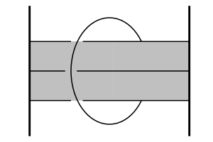
Figure 21. Band sum

Proof of Proposition 2.2.1.

We can reinterpret the fiber sum as the result (on the boundary) of adding a $5$-dimensional toric $1$-handle (a $T^{2}\times D^{2}\times I$) to $X\times I$ so that the attaching region, $T^{2}\times D^{2}\times\pm 1$ is identified with the normal bundles to $T_{1}$ and $T_{2}$ with their chosen framing. This results in deleting the two $T^{2}\times D^{2}$s and replacing them with a $T^{2}\times\partial D^{2}\times I$. This identification is determined by choice of framings for $T_{1},T_{2}$ and a diffeomorphism $\phi$ between them.

Choose a factorization $T_{1}\cong_{\phi}T_{2}\cong S^{1}_{\alpha}\times S^{1}_{\beta}$ so that the $S^{1}_{\alpha}$ factor is $\partial A$ in both $T_{i}$s. The critical $T^{2}$ for the $5$-dimensional toric handle is identified with the $T_{i}$s by the gradient flow. Pick a perfect Morse function on $S^{1}_{\beta}$ and perturb the Morse-Bott function on the $5$-dimensional handle by an extension of it. This gives us a reinterpretation of the $5$-dimensional toric $1$-handle as two round ($S^{1}$) handles — a round $2$-handle and a round $1$-handle — corresponding to the critical points of the Morse function on $S^{1}_{\beta}$.

Consider the round $1$-handle first. Such a handle is a $S^{1}\times D^{3}\times I$ so that it attaches along $S^{1}\times D^{3}\times\pm 1$. By construction, the two $S^{1}\times D^{3}$s are neighborhoods of the components of $\partial A$, with framing given by the inward normal along $A$, a vector field along $\partial A$ parallel to $T_{i}$, and a third vector field defined by orthogonality to these and the tangent space to $\partial A$.

Consider a neighborhood of $A$ which is $S^{1}$ equivariant, matching the $S^{1}$ equivariance of $A=I\times S^{1}$. When small, such a neighborhood is diffeomorphic to $S^{1}$ times the “H” in Figure 21. (The vertical lines are in $T_{i}$; the horizontal, slices of $A$.) Attaching the round $1$-handle is the same as (equivariantly) self-connect summing at the places where the vertical lines intersect the horizontal core of the band. In each $3$-manifold slice, this is equivalent to performing zero surgery on the loop linking the band in Figure 21. Then, in turn, this gives us a square zero torus $L$ and a surgery to perform on it within the neighborhood of $A$.

Now, a $5$-dimensional round $2$-handle is a $S^{1}\times D^{2}\times D^{2}$ attached along $S^{1}\times D^{2}\times\partial D^{2}$. Outside of the neighborhood of $A$, the attaching torus is equal to the $T_{i}$. (two annuli) Inside the neighborhood of $A$, the attaching torus $T$ is given by $S^{1}$ times the boundary of the band in Figure 21. (two more annuli) The framing of this torus is given by the framings of the $T_{i}$ outside the neighborhood of $A$ and by the inward normal to the band on (each slice of) the inside. This can be seen by band summing pushoffs of the $T_{i}$. (By hypothesis, $A$ has zero winding with respect to our framing so this can be done by band summing in the $S^{1}$ trivialization. ) $T$ inherits a factorization $S^{1}_{a}\times S^{1}_{b}$ from the $T_{i}$ by noting that the $S^{1}_{\alpha}$ factors of the $T_{i}$ survive and that the $S^{1}_{\beta}$ factors are themselves band summed. Attaching the round $2$-handle then performs a surgery on this torus which sends $\partial D^{2}$ to the $S^{1}_{b}$ factor. ∎

2.2.1. $4$-Dimensional Hoste Move for a Twin and Torus

Let us now examine how Proposition 2.2.1 can be described in terms of surgery information on projections. First we will look at the case when the tori come from surgeries on a twin and a torus.

Let $X$ be the result of standard surgery on a ribbon twin ${\mathbb{T}\mathrm{w}}$ and $(0,0)$ surgery on a ribbon torus $T$ in $S^{4}$, both specified by a virtual knot diagram as in sections 1.6 and 1.7. Note that the cores $T_{\mathbb{T}\mathrm{w}},T_{T}$ of each surgery inherit preferred framings from their surgery description.

Suppose that ${\mathbb{T}\mathrm{w}}$ and $T$ have a classical knot crossing in the virtual knot diagram and hence a ribbon intersection. Then, in a projection to $\mathbb{R}^{3}$, there is a neighborhood as in Figure 22. Consider the annuli shown in the figure. Each of these annuli are isotopic. This can be seen by the fact that on the left of each picture, the horizontal surface overcrosses the vertical surface so the annulus must lie completely under the horizontal surface to the left of the ribbon singularity. Thus we can isotope the annulus freely on the left of the ribbon singularity. Similarly, on the right the annulus lies completely above the horizontal surface and so we can isotope it freely on that side.

Now let $B$ be the particular representation of the annulus corresponding to the particular orientations of the virtual knot crossing depicted below it. Now, $B$ connects an equator $\gamma_{\mathbb{T}\mathrm{w}}$ to one of $K_{i}$ in ${\mathbb{T}\mathrm{w}}=K_{1}\operatorname*{\cup}K_{2}$ to a essential curve $\gamma_{T}$ on the torus. Since we have done $(0,0)$ surgery on the torus (in virtual knot notation), the surgery curve (in the projection notation) meets $\gamma_{T}$ once.

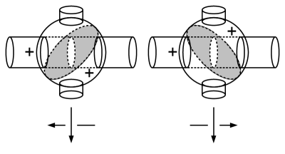
Figure 22. Annulus $B$ used for smoothing

The method of constructing $B$ ensures that $\partial B$ consists of essential curves on the cores of the twin and torus surgeries when $B$ is extended by the projection to the surgered manifold. This means that we can apply proposition 2.2.1 once we have chosen the diffeomorphism $\phi$ between $T_{\mathbb{T}\mathrm{w}},T_{T}$. We have already required that $\phi$ identify the components of $\partial B$. $\phi$ is then determined when we require that it identify the following:

1. the projection to $T_{T}$ of $\text{pt}_{1}\times\partial D^{2}$, where $\text{pt}_{1}\in T$, $T\times D^{2}\subset S^{4}$ the normal bundle, and

2. the projection to $T_{\mathbb{T}\mathrm{w}}$ of $\text{pt}_{2}\times\partial D^{2}$, where $\text{pt}_{2}\in{\mathbb{T}\mathrm{w}}\setminus(S^{2}\text{ intersection points})$ and lies in the $S^{2}$ which does not contain the preimage of the double points. $\partial D^{2}$ is the boundary of the fiber of the normal bundle to this $S^{2}$.

With this data fixed, proposition 2.2.1 can be applied. The result is that

$$X\setminus(\nu T_{{\mathbb{T}\mathrm{w}}}\operatorname*{\cup}\nu T_{T}))=S^{4}\setminus(\nu{\mathbb{T}\mathrm{w}}\operatorname*{\cup}\nu T)$$

sewn up by $\phi$ is diffeomorphic to

$$S^{4}\setminus(\nu({\mathbb{T}\mathrm{w}}\operatorname*{\#}_{B}T)\operatorname*{\cup}\tau)\operatorname*{\cup}T^{2}\times D^{2}\operatorname*{\cup}T^{2}\times D^{2}$$

where

1. ${\mathbb{T}\mathrm{w}}\operatorname*{\#}_{B}T$ denotes the “band sum” of ${\mathbb{T}\mathrm{w}}$ and $T$ along $B$,

2. the first $T^{2}\times D^{2}$ is glued to $\partial\nu({\mathbb{T}\mathrm{w}}\operatorname*{\#}_{B}T)$ by the standard surgery on twins,

3. $\tau$ is the torus given by the loop in Figure 21, and

4. the second $T^{2}\times D^{2}$ is glued to $\partial\nu\tau$ so that $\partial D^{2}$ goes to the nullhomologous pushoff of the loop in Figure 21.

Finally, we can isotopy this region in ${\mathbb{T}\mathrm{w}}\operatorname*{\#}_{B}T$ to be as shown in one of the pictures in the top row of Figure 23. The appropriate smoothing depends on the orientation of the horizontal surface and corresponds to the selection of band previously. In Figure 23, the correspondence of the orientation of the horizontal surface to the virtual knot diagrams is show by the original diagrams to the lower left of each smoothing and the smoothed virtual knot diagrams to the lower right.

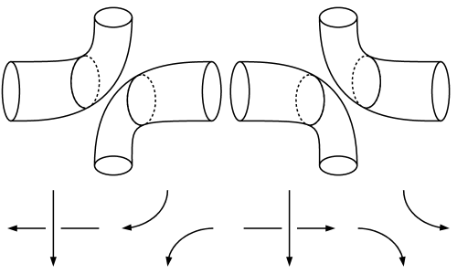
Figure 23. Two smoothings of the intersection on Figure 22 with corresponding virtual knot diagrams

2.2.2. $4$-Dimensional Hoste Move for two Tori

We will require the Hoste Move between two tori in only one case. Suppose that both tori lie in a neighborhood diffeomorphic to $S^{1}\times D^{3}$ so that in each $\theta\times D^{3}$ the tori are as shown in Figure 24. The we only need to describe one aspect of the $3$-dimensional local picture — the gluing map for the sewn up exterior for the right hand side of Figure 24. This map is given by identifying meridians to each loop and the pushoffs along the obvious once punctured discs to each.

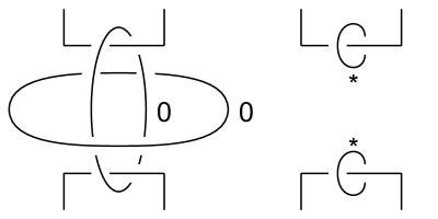
Figure 24. $S^{1}$ times the left is $S^{1}$ times the right with the two starred tori sewn up

2.3. $4$-Dimensional Crossing Change

Consider a classical crossing in a virtual knot diagram for a twin and/or a torus and the corresponding annulus from Figure 25. Notice that the correspondence is reversed from that of the $4D$ Hoste move. As before, both bands shown are isotopic. Push the horizontal surface along the annulus in Figure 25 to get the configuration in Figure 26.

Figure 25. Annulus $B$ used for crossing change

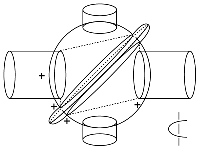
Figure 26. Diagram obtained from the first picture in Figure 25 by pushing horizontal tube along band, over crossing the vertical tube in the two new sets of double points. The new pair of crossings is locally modeled on $S^{1}$ times the diagram in the lower right. The diagram corresponding to the second picture in Figure 25 is similar.

Focus our attention to the lower of the two new loops of crossings in Figure 26 (or the corresponding picture for the other band.) Call this crossing $C$. Local to $C$, we have the model of $S^{1}$ times a $3$-dimensional oriented knot crossing. Note that if we form an annulus by taking a path from the lower to the upper double point in each $3$-manifold picture, we get an annulus $A$ which is isotopic to the annulus $B$ from before.

Perform one of the surgeries on a torus indicated by the $3$-dimensional pictures in Figure 27 localized at $C$ in Figure 26 (or the corresponding picture for the other band.) The appropriate surgery is the top for the first picture of Figure 25 and the lower for the second. This changes the crossing $C$ from an overcrossing of the horizontal surface to an under crossing, resulting in Figures 28 and 29. Finally, we perform the isotopies indicated in these figures and see that our result has changed the crossing type from a classical $+$ to $-$ or from a classical $-$ to $+$ in the virtual knot diagram.

It is important to note that the torus which we have surgered is isotopic to the surgered torus $\tau$ of section 2.2.1. We identify the two via the isotopy of the band $B$.

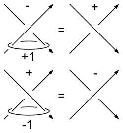
Figure 27. Isotopy in $3$-dimensional picture

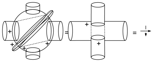
Figure 28. Isotopy of first picture in Figure 25 after surgery and the corresponding virtual knot crossing of result

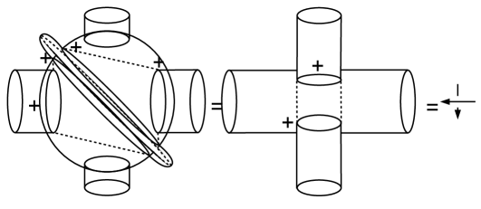
Figure 29. Isotopy of second picture in Figure 25 after surgery and the corresponding virtual knot crossing of result

3. Calculation of the Invariant for Certain Ribbon Twins

Consider a twin ${\mathbb{T}\mathrm{w}}=K_{1}\cup K_{2}$ given by a virtual knot presentation and the manifold $X({\mathbb{T}\mathrm{w}})=E(2)_{{\mathbb{T}\mathrm{w}}}$. Suppose that the virtual knot presentation for $K_{1}$ contains a classical crossing; so $K_{1}$ has a ribbon intersection with itself. Let ${\mathbb{T}\mathrm{w}}_{+}$, ${\mathbb{T}\mathrm{w}}_{-}$ and ${\mathbb{T}\mathrm{w}}_{0}$ be the results of replacing the crossing in the virtual knot diagram with the three options in Figure 30. Note that ${\mathbb{T}\mathrm{w}}_{0}$ will actually be a twin and a torus.

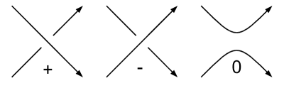
Figure 30.

Consider the square zero torus $\tau$ from the previous sections. Now, $\partial\nu\tau$ admits a decomposition $\partial\nu\tau=S^{1}_{\alpha}\times S^{1}_{\beta}\times S^{1}_{\gamma}$ from it lying in the $S^{1}$ equivariant neighborhood of the annulus $B$. Namely, in each $3$-manifold slice of the neighborhood, $\tau$ is given by a loop $\alpha$ linking the slice of $B$ once. Then $S^{1}_{\alpha}\times S^{1}_{\beta}=\tau$ where $\beta$ is $\text{pt}\times S^{1}$ in the equivariant neighborhood of $B$. Finally $S^{1}_{\gamma}=\partial D^{2}$ finishes the decomposition.

Log transform surgery on $\tau$ is defined by removing $\nu\tau\cong T^{2}\times D^{2}$ and replacing with another copy of $T^{2}\times D^{2}$. Such a surgery is uniquely determined up to diffeomorphism by the image of $\partial D^{2}$ in $\partial\nu\tau\cong T^{3}$. Using our decomposition above, we can describe such a surgery by a triplet of integers $(a,b,c)$ with no common factor. Such a triplet gives specifies the isotopy type of the curve to which we will glue $\partial D^{2}$. We will write $X_{\tau(a,b,c)}$ for the result of the $(a,b,c)$ log transform surgery on $X$.

From section 2.3 we see that we can move from ${\mathbb{T}\mathrm{w}}_{-}$ to ${\mathbb{T}\mathrm{w}}_{+}$ by surgery on $\tau\subset S^{4}\setminus{\mathbb{T}\mathrm{w}}_{-}$ which in each $3$-manifold slice is $+1$ surgery on the loop which gives $\tau$. Thus we can move from ${\mathbb{T}\mathrm{w}}_{-}$ to ${\mathbb{T}\mathrm{w}}_{+}$ by a $(0,1,1)$ log transform on $\tau$. Note that $(0,0,1)$ surgery on $\tau$ is the identity.

Morgan, Mrowka, and Szabo’s formula in [MMS97] then gives

$$SW(E(2)_{{\mathbb{T}\mathrm{w}}_{+}})=SW(E(2)_{{\mathbb{T}\mathrm{w}}_{-}})+SW(E(2)_{{\mathbb{T}\mathrm{w}}_{-},\tau(0,1,0)})$$

Now by our description in section 2.2.1, $E(2)_{{\mathbb{T}\mathrm{w}}_{-},\tau(0,1,0)}$ is the sewn up twin/torus exterior of ${\mathbb{T}\mathrm{w}}_{0}$ fiber summed to $E(2)$. Thus, by our definition of $I$,

$$SW(E(2)_{{\mathbb{T}\mathrm{w}}_{-},\tau(0,1,0)})=(t-t^{-1})I({\mathbb{T}\mathrm{w}}_{0}),$$

while

$$I({\mathbb{T}\mathrm{w}}_{+})=SW(E(2)_{{\mathbb{T}\mathrm{w}}_{+}})$$

and

$$I({\mathbb{T}\mathrm{w}}_{-})=SW(E(2)_{{\mathbb{T}\mathrm{w}}_{-}}).$$

Therefore,

$$I({\mathbb{T}\mathrm{w}}_{+})=I({\mathbb{T}\mathrm{w}}_{-})+(t-t^{-1})I({\mathbb{T}\mathrm{w}}_{0})$$

Now consider a twin ${\mathbb{T}\mathrm{w}}=K_{1}\cup K_{2}$ and torus $\mathbb{T}$ given by a virtual knot presentation and the manifold $X({\mathbb{T}\mathrm{w}})=E(2)_{{\mathbb{T}\mathrm{w}}}$. Suppose that the virtual knot presentation contains a classical crossing between $K_{1}$ and $\mathbb{T}$; so $K_{1}$ has a ribbon intersection with $T$. Let ${\mathbb{T}\mathrm{w}}_{+}$, ${\mathbb{T}\mathrm{w}}_{-}$ and ${\mathbb{T}\mathrm{w}}_{0}$ be the results of replacing the crossing in the virtual knot diagram with the three options in Figure 30. Note that ${\mathbb{T}\mathrm{w}}_{\pm}$ will each be a twin and a torus while ${\mathbb{T}\mathrm{w}}_{0}$ will be a single twin.

As before, we consider the torus $\tau\subset S^{4}\setminus{\mathbb{T}\mathrm{w}}_{-}$. From section 2.3 we see that we can move from ${\mathbb{T}\mathrm{w}}_{-}$ to ${\mathbb{T}\mathrm{w}}_{+}$ by surgery on $\tau\subset S^{4}\setminus{\mathbb{T}\mathrm{w}}_{-}$ which in each $3$-manifold slice is $+1$ surgery on the loop which gives $\tau$. Thus we can move from ${\mathbb{T}\mathrm{w}}_{-}$ to ${\mathbb{T}\mathrm{w}}_{+}$ by a $(0,1,1)$ log transform on $\tau$. Note that $(0,0,1)$ surgery on $\tau$ is the identity.

Morgan, Mrowka, and Szabo’s formula in [MMS97] then gives

$$SW(E(2)_{{\mathbb{T}\mathrm{w}}_{+}})=SW(E(2)_{{\mathbb{T}\mathrm{w}}_{-}})+SW(E(2)_{{\mathbb{T}\mathrm{w}}_{-},\tau(0,1,0)})$$

Now, since each ${\mathbb{T}\mathrm{w}}_{\pm}$ are composed of a torus and a twin, the manifolds $E(2)_{{\mathbb{T}\mathrm{w}}_{\pm}}$ are each sewn up twin/torus exteriors fiber summed to $E(2)$. Thus $SW(E(2)_{{\mathbb{T}\mathrm{w}}_{\pm}})=(t-t^{-1})I({\mathbb{T}\mathrm{w}}_{\pm})$.

Nearby $\tau$ we have a local model for ${\mathbb{T}\mathrm{w}}_{-}$ given in the left picture of Figure 31. If we perform the $4D$ Hoste move on $E(2)_{{\mathbb{T}\mathrm{w}}_{-},\tau(0,1,0)}$ at an annulus equal to $S^{1}$ times the horizontal line in this picture, we obtain the picture to the right in Figure 31.

Figure 31. Hoste move nearby $\tau$

Note that this picture is identical to that of Figure 24. Applying the version of the $4D$ Hoste move from section 2.2.2, we get a local picture equal to that in the right hand side of Figure 24. The tori in this picture are each isotopic to the torus $\partial D^{2}_{1}\times\partial D^{2}_{2}$ – where $\partial D^{2}_{i}$ is the normal bundle to $K_{i}$, the knots which comprise ${\mathbb{T}\mathrm{w}}_{0}$. This torus can also be described as one of the components of $\partial\nu K_{1}\cap\partial\nu K_{2}$. In the fiber sum manifold, $E(2)_{{\mathbb{T}\mathrm{w}}_{-},\tau(0,1,0)}$, each torus we have just described is isotopic to the fiber $F$. Thus, $E(2)_{{\mathbb{T}\mathrm{w}}_{-},\tau(0,1,0)}$ is diffeomorphic to $E(2)_{{\mathbb{T}\mathrm{w}}_{0}}\operatorname*{\#}_{F=F^{\prime}}$. Therefore, $SW(E(2)_{{\mathbb{T}\mathrm{w}}_{-},\tau(0,1,0)})=(t-t^{-1})^{2}SW(E(2)_{{\mathbb{T}\mathrm{w}}_{0}})$ so

$$SW(E(2)_{{\mathbb{T}\mathrm{w}}_{+}})=SW(E(2)_{{\mathbb{T}\mathrm{w}}_{-}})+(t-t^{-1})^{2}SW(E(2)_{{\mathbb{T}\mathrm{w}}_{0}})$$

and

$$(t-t^{-1})I({\mathbb{T}\mathrm{w}}_{+})=(t-t^{-1})I({\mathbb{T}\mathrm{w}}_{-})+(t-t^{-1})^{2}I({\mathbb{T}\mathrm{w}}_{0})$$

so

$$I({\mathbb{T}\mathrm{w}}_{+})=I({\mathbb{T}\mathrm{w}}_{-})+(t-t^{-1})I({\mathbb{T}\mathrm{w}}_{0})$$

3.1. Relation to Giller’s polynomial

Recall the definition of Giller’s polynomial given by Equations (2), (3), and (4). These are the Conway-style relation, the value on the unknotted sphere, and the vanishing of the polynomial for split links, respectively. We now discuss similar results for our invariant.

That $I({\mathbb{T}\mathrm{w}}_{std})=1$ was shown at Equation (1).

Suppose that ${\mathbb{T}\mathrm{w}}=K_{1}\operatorname*{\cup}K_{2}$ and $T$ are ribbon with a virtual knot presentation which is split or only has pairwise virtual crossings. Then using the virtual Reidemeister moves of Figures 12 and 13, we can separate ${\mathbb{T}\mathrm{w}}$ and $T$. This means that the projections of ${\mathbb{T}\mathrm{w}}$ and $T$ are separated by an $S^{3}$. So ${\mathbb{T}\mathrm{w}}$ and $T$ are separated by an $S^{3}$. This means that the manifold formed by surgering ${\mathbb{T}\mathrm{w}}$ and $T$ is a connected sum. Now, on the $T$ side of the connected sum, the intersection form on $H_{2}$ will be a hyperbolic pair as will the intersection form on the side given by surgery on ${\mathbb{T}\mathrm{w}}$. Thus we are given a manifold which is the connected sum of two manifolds each with $b_{+}>0$. Therefore, the Seiberg-Witten invariant of this surgery vanishes. It follows that $SW(E(2)_{{\mathbb{T}\mathrm{w}},T})=0$ and that

(5) $$I({\mathbb{T}\mathrm{w}},T)=0\text{ for }{\mathbb{T}\mathrm{w}},T\text{ split.}$$

Now let us consider the Conway-style relation for Giller’s polynomial we initially discussed in Section 1.8. This relation involves crossing changes and resolution at individual loops of double points. Now, in our crossing change surgery, we had a similar action of changing the lower crossing from Figure 26. In the diagrams for our $4D$ Hoste move, we took a different local projection to illustrate the appropriate surgery. However, smoothing the lower crossing from Figure 26 also yields a smoothing in the virtual knot diagram.

In other words, selecting a particular set of double points to apply the relation in Equation (2) to, $\Delta_{G}({\mathbb{T}\mathrm{w}})$ computes $I({\mathbb{T}\mathrm{w}})$. Therefore, $\Delta_{G}({\mathbb{T}\mathrm{w}})=I({\mathbb{T}\mathrm{w}})$ for ribbon knots. We cannot make a stronger statement of equality however, as the relation from Equation (2) allows us to move into configurations of surfaces which are inaccessible to the invariant $I$.

3.2. The Class of Ribbon Twins

We now make some remarks on computations.

Now suppose that ${\mathbb{T}\mathrm{w}}=K_{1}\operatorname*{\cup}K_{2}$ is ribbon with a virtual knot presentation which only has virtual crossings. Then we can use the virtual Reidemeister moves $B$ and $F$ from Figures 12 and 13 to completely unknot the diagram for ${\mathbb{T}\mathrm{w}}$. Therefore, ${\mathbb{T}\mathrm{w}}={\mathbb{T}\mathrm{w}}_{std}$ and so $I({\mathbb{T}\mathrm{w}})=I({\mathbb{T}\mathrm{w}}_{std})=1$.

Suppose that ${\mathbb{T}\mathrm{w}}=K_{1}\operatorname*{\cup}K_{2}$ is a twin possibly with accompanying torus $T$ with the configuration ribbon. Suppose that we reverse the orientation of one of the $K_{i}$ or of $T$. This reverses the orientation of the torus $T_{\mathbb{T}\mathrm{w}}$ (or $T_{T}$) and induces a chance in homology orientation from the change of sign in pairing with $T_{\mathbb{T}\mathrm{w}}$. Then, if $\widehat{{\mathbb{T}\mathrm{w}}}=\overline{K_{1}}\operatorname*{\cup}K_{2}$, $I(\widehat{{\mathbb{T}\mathrm{w}}})=-I({\mathbb{T}\mathrm{w}})$. Similarly, $I({\mathbb{T}\mathrm{w}},\overline{T})=-I({\mathbb{T}\mathrm{w}},T)$.

Currently, the author is unaware if crossings can be chosen so that the tree of terminates in standard twins and unlinked twin/torus pairs. The previous work of Fintushel and Stern guarantees that the process terminates when $K_{1}$ in ${\mathbb{T}\mathrm{w}}=K_{1}\operatorname*{\cup}K_{2}$ is knotted with only classical crossings and $K_{2}$ is unknotted with no ribbon intersections with $K_{1}$. The presence of virtual crossings in the diagrams complicates the general case. Additionally, the author has yet to find a general method of dealing with ribbon intersections between the $K_{i}$.

However, there seem to be a fairly large number of new examples which we may compute using the current tools. The first we will compute is the twin version of the example from Giller’s paper. Call this twin ${\mathbb{T}\mathrm{w}}_{G}$. This was encountered previously in Figure 16.

Follow the computation through Figures 32, 33, 34, and 35. In Figure 35, we arrive at configurations $C,D,E,$ and $F$. Here $C$ and $F$ are isotopic to standard twins, so $I(C)=I(F)=1$. The other configurations $D,E$ differ by the orientation of the torus and so $I(D)=-I(E)$. Therefore,

$$I({\mathbb{T}\mathrm{w}}_{G}) = I(A)+(t-t^{-1})I(B)$$

$$= I(C)+(t-t^{-1})I(D)+(t-t^{-1})I(E)+(t-t^{-1})^{2}I(F)$$

$$= 1+0+(t-t^{-1})^{2}$$

$$= t^{-2}-1+t^{2}$$

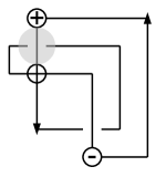
Figure 32. Giller Twin ${\mathbb{T}\mathrm{w}}_{G}$ with highlighted crossing

Figure 33. $I({\mathbb{T}\mathrm{w}}_{G})=I(A)+(t-t^{-1})I(B)$

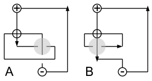
Figure 34. Isotopy of $A$ and $B$ from Figure 33 with highlighted crossings

Figure 35. $I({\mathbb{T}\mathrm{w}}_{G})=I(C)+(t-t^{-1})I(D)+(t-t^{-1})I(E)+(t-t^{-1})^{2}I(F)$

Now let us look at the twin in Figure 36, a twin in which both $2$-knots are unknots but which pairwise have ribbon intersections. Call this twin ${\mathbb{T}\mathrm{w}}_{U}$. Our current tools do not allow us to deal directly with pairwise ribbon intersections.

Follow the computation through Figures 37, 38, and 39. We arrive at configurations $H,K,$ and $L$. Here $H$ and $L$ are isotopic to standard twins, so $I(H)=I(L)=1$. The other configurations $K$ contains a separated torus so $I(K)=0$. Therefore,

$$I({\mathbb{T}\mathrm{w}}_{U}) = I(H)-(t-t^{-1})I(J)$$

$$= I(H)-(t-t^{-1})I(K)+(t-t^{-1})^{2}I(L)$$

$$= 1+0+(t-t^{-1})^{2}$$

$$= t^{-2}-1+t^{2}$$

Finally, we remark on uniqueness and related topics. In what is our Artin spun case, Fintushel and Stern have conjectured that their knot surgery construction yields nondiffeomorphic manifolds for “essentially different” knots. (Here, “essentially different” means that two knots are not isotopic, they are not mirrors, nor they isotopic under mirroring of connect-summands.) The Alexander polynomial does not completely distinguish knots however, so the Seiberg-Witten invariants in their current form do not shed any light on their conjecture. Similarly, it seems doubtful that the manifolds $E(2)_{{\mathbb{T}\mathrm{w}}_{G}}$ and $E(2)_{{\mathbb{T}\mathrm{w}}_{U}}$ are diffeomorphic, but with the Seiberg-Witten invariants being equal, we have no obvious way in which to distinguish them. In particular, it seems possible that $E(2)_{{\mathbb{T}\mathrm{w}}_{U}}$ is diffeomorphic to $E(2)_{{\mathbb{T}\mathrm{w}}_{K}}$ where ${\mathbb{T}\mathrm{w}}_{K}$ is the Artin spin of the left handed trefoil.

Also, results of C. Taubes in [Tau94] show that a manifold $X$ with $b_{+}>2$ admits a symplectic form, the leading term in $SW(X)$ will have coefficient equal to one. The converse to this statement is known to be false by work of Fintushel and Stern in [FS97]. In the classical (or Artin spun) case, it is possible to construct a symplectic form on $E(2)_{{\mathbb{T}\mathrm{w}}}$ when the classical knot $K$ from which ${\mathbb{T}\mathrm{w}}$ is constructed is a fibered knot. While it may be possible to rephrase this construction in terms of twins, it is unclear what topological conditions are required on ${\mathbb{T}\mathrm{w}}$ to achieve the same result. (A sufficient condition is that $S^{4}_{{\mathbb{T}\mathrm{w}}}$ fibers over $T^{2}$ or $S^{2}$.)

We then ask, do $E(2)_{{\mathbb{T}\mathrm{w}}_{G}},E(2)_{{\mathbb{T}\mathrm{w}}_{U}}$ admit symplectic forms? What conditions on the exterior of the twin guarantee a symplectic form?

Figure 36. A twin in which both $2$-knots are unknots

Figure 37. A negative crossing from Figure 36

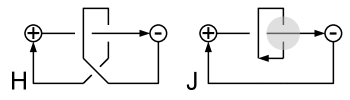
Figure 38. $I({\mathbb{T}\mathrm{w}}_{U})=I(H)-(t-t^{-1})I(J)$

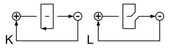
Figure 39. $I(J)=I(K)-(t-t^{-1})I(L)$

References

- [AC59] J. J. Andrews and M. L. Curtis. Knotted 2-spheres in the 4-sphere. Ann. of Math. (2), 70:565–571, 1959.
- [Art26] E. Artin. Zur isotopie zweidimensionalen flächen im . Abh. Math. Sem. Univ. Hamburg, 4:174–177, 1926.
- [Fox66] R. H. Fox. Rolling. Bull. Amer. Math. Soc., 72:162–164, 1966.
- [FS97] R. Fintushel and R. J. Stern. Surfaces in -manifolds. Math. Res. Lett., 4(6):907–914, 1997.
- [FS98] R. Fintushel and R. Stern. Knots, links, and -manifolds. Invent. Math., 134(2):363–400, 1998.
- [Gil82] C. A. Giller. Towards a classical knot theory for surfaces in . Illinois J. Math., 26(4):591–631, 1982.
- [GK78] D. L. Goldsmith and L. H. Kauffman. Twist spinning revisited. Trans. Amer. Math. Soc., 239:229–251, 1978.
- [Gor76] C. McA. Gordon. Knots in the -sphere. Comment. Math. Helv., 51(4):585–596, 1976.
- [Gra77] A. Gramain. Sur le groupe fundamental de l’espace des noeuds. Ann. Inst. Fourier (Grenoble), 27(3):ix, 29–44, 1977.
- [Hos84] J. Hoste. Sewn-up -link exteriors. Pacific J. Math., 112(2):347–382, 1984.
- [Lit79] R. A. Litherland. Deforming twist-spun knots. Trans. Amer. Math. Soc., 250:311–331, 1979.
- [Mar92] Y. Marumoto. Stable equivalence of ribbon presentations. J. Knot Theory Ramifications, 1(3):241–251, 1992.
- [MMS97] J. W. Morgan, T. S. Mrowka, and Z. Szabó. Product formulas along for Seiberg-Witten invariants. Math. Res. Lett., 4(6):915–929, 1997.
- [Mon83] J. M. Montesinos. On twins in the four-sphere. I. Quart. J. Math. Oxford Ser. (2), 34(134):171–199, 1983.
- [Mon84] J. M. Montesinos. On twins in the four-sphere. II. Quart. J. Math. Oxford Ser. (2), 35(137):73–83, 1984.
- [Rol76] D. Rolfsen. Knots and links. Publish or Perish Inc., Berkeley, Calif., 1976. Mathematics Lecture Series, No. 7.
- [Sat00] S. Satoh. Virtual knot presentation of ribbon torus-knots. J. Knot Theory Ramifications, 9(4):531–542, 2000.
- [Tau94] C. H. Taubes. The Seiberg-Witten invariants and symplectic forms. Math. Res. Lett., 1(6):809–822, 1994.
- [Yaj64] T. Yajima. On simply knotted spheres in . Osaka J. Math., 1:133–152, 1964.
- [Zee65] E. C. Zeeman. Twisting spun knots. Trans. Amer. Math. Soc., 115:471–495, 1965.