Head shock vs Mach cone:
azimuthal correlations from 2$\rightarrow$3 parton processes
in relativistic heavy-ion collisions

Abstract

We study the energy momentum deposited by fast moving partons within a medium using linearized viscous hydrodynamics. The particle distribution produced by this energy momentum is computed using the Cooper-Frye formalism. We show that for the conditions arising in heavy-ion collisions, energy momentum is preferentially deposited along the head shock of the fast moving partons. We also show that the double hump in the away side of azimuthal correlations can be produced by two (instead of one) away side partons that deposit their energy momentum along their directions of motion. These partons are originated in the in-medium hard scattering in $2\to 3$ processes. We compare the results of the analysis to azimuthal angular correlations from PHENIX and show that the calculation reproduces the data systematics of a decreasing away side correlation when the momentum of the associated hadron becomes closer to the momentum of the leading hadron. This scenario seems to avoid the shortcomings of the Mach cone as the origin of the double-hump structure in the away side.

I Introduction

Azimuthal angular correlations have provided a powerful testing ground to elucidate the propagation properties of fast partons within the medium created in high-energy heavy-ion reactions STAR ; PHENIX . The main features of these correlations can be summarized as follows: when the leading and the away side particles have similar momenta, the correlation shows a suppression of the away side peak, compared to proton collisions at the same energies. However, when the momentum difference between leading and away side particles increases, either a double peak or a broadening of the away side peak appears, whereas neither of these are present in proton collisions at the same energies azcor . The peak region is known as the shoulder and the region between the peaks is known as the head. For low-momentum particles, the jet multiplicity is larger in the shoulder than in the head region PHENIX .

Because the structures in the away side are best seen for low momentum particles, there were explanations based on the emission of sound modes caused by one fast moving parton Casalderrey ; Renk , the so-called Mach cones. Nevertheless, it has been argued that such interpretation is fragile, since the jet-medium interaction produces also a wake whose contribution cannot be ignored Casalderrey2 ; Torrieri . Furthermore, it was recently shown that it is unlikely that the propagation of one high-energy particle through the medium leads to a double-peak structure in the azimuthal correlation in a system of the size and finite viscosity relevant for heavy-ion collisions, since the energy momentum deposition in the head shock region is strongly forwardpeaked Bouras . Moreover, by using a realistic multiple-gluon emission for the parton shower produced by an in-medium moving parton, the overlapping perturbations in very different spatial directions wipe out any distinct Mach cone structure  Neufeld3 .

The more widely accepted explanation for the double peak or broadening of the away side is given nowadays in terms of initial state fluctuations of the matter density in the colliding nuclei. These fluctuations are then shown to give rise to an anisotropic flow of partially equilibrated, low-momentum particles, within the bulk medium. Hydrodynamic descriptions of this scenario have for instance successfully reproduced the experimental $v_{3}$ v3 . However, it has also been shown that there is a strong connection between the observed away side structures and the medium’s path length pathlength . The connection is expressed through the dependence of the azimuthal correlation on the trigger particle direction with respect to the event plane in such a way that, for selected trigger and associated particle momenta, the double peak is present (absent) for out-of-plane (in-plane) trigger particle direction. A final-state effect rather than an an initial state one seems more consistent with this observation.

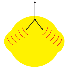
Figure 1: (Color on line) Schematic representation of the possible origin of the away side double hump. The left panel illustrates the common picture whereby one away side parton deposits energy momentum, exciting the sound modes and producing a Mach cone. The right panel illustrates our approach whereby two away side partons each generate head-shock and deposit energy momentum preferentially along their directions of motion.

The medium’s response to a fast moving parton can be described by the energy and momentum that the parton deposits. This energy momentum is then converted into particles upon hadronization. When the interaction produces low-momentum particles, a hydrodynamic description of the medium’s response seems appropriate. In this framework, it is natural to explore the types of medium excitations generated by fast moving partons and the way these in turn are responsible for the shape of the away side in the angular correlations. When the sound (that is, the longitudinal modes) are prominently excited, the double peak in the away side could emerge as a Mach cone structure, that is, as energy momentum mainly deposited on the sides of the path traveled by the parton. This is illustrated in the left-hand panel of Fig. 1. However, when the modes that get prominently excited are the wake (that is, the transverse modes), energy and momentum is preferentially deposited along the direction of the travelling parton. If a double peak is to emerge, the alternative scenario is that the structure is produced by two travelling partons in the away side. This is illustrated in the right-hand panel of Fig. 1.

Two partons in the away side are produced in processes where two initial-state partons scatter into three final-state ones, the so-called $2\rightarrow 3$ processes. In this case the cross section is smaller than the one for $2\rightarrow 2$ processes, at least by one power of $\alpha_{s}$. However, consider a scattering event that deposits a given amount of energy in the away side. If such an event comes from a $2\rightarrow 2$ process, the away side parton will have a larger energy than each of the two partons, when these last come from a $2\rightarrow 3$ process. Because the parton distribution is a fast falling function of the parton energy, the extra power of $\alpha_{s}$ is partially compensated by the larger abundance of partons with smaller energy. This is illustrated in Fig. 2. For $2\rightarrow 3$ processes, when the dominant energy momentum deposition happens through transverse modes, conservation of momentum at the parton level gives rise to a distinctive angular dependence in the azimuthal correlation whereby, the angular difference between the peaks in the away side is close to $2\pi/3$ rad.

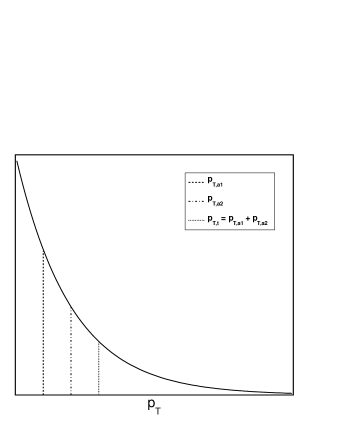
Figure 2: Schematic representation of how a single away side parton is less abundantly produced than two away side partons carrying the same total momentum, given that the momentum distribution function rapidly decays with momentum.

The computation of hadron events produced by $2\rightarrow 3$ parton processes in the context of azimuthal correlation functions was put forward and explored in Refs. Ayala1 ; Ayala2 , using the leading order QCD matrix elements. Those studies were made for fragmentation outside the medium. In this work we compute the hadron multiplicity produced by two partons in the away side coming from $2\rightarrow 3$ processes for the case where all its energy momentum is deposited into the medium. We use linearized viscous hydrodynamics to compute the medium’s response. The work is organized as follows: In Sec. II we first review the general framework to compute the particle distribution stemming from a given energy momentum deposited by a fast moving parton within the medium, using linearized viscous hydrodynamics. This energy momentum is then converted into a parton multiplicity using the Cooper-Frye formalism Cooper-Frye . We discuss the different shapes for the azimuthal correlations that are obtained when varying the strength of the wake and sound mode contributions. In Sec. III we solve the hydrodynamic equations for the transverse and longitudinal modes. We work in the limit where the parton’s velocity is larger than the sound velocity. In Sec. IV we use these solutions to compute the azimuthal correlations by convoluting the pQCD probability to produce two away side partons in $2\rightarrow 3$ processes with the multiplicity obtained from the excess of energy momentum produced by the moving partons followed by fragmentation. We finally summarize and conclude in Sec. V.

II Particle distribution

We compute the particle’s multiplicity as given by the Cooper-Frye formula

$$E\frac{dN}{d^{3}p}=\frac{1}{(2\pi)^{3}}\int d\Sigma_{\mu}p^{\mu}[f(p\cdot u)-f(p_{0})],$$ (1)

where $f(p\cdot u)-f(p_{0})$ is the phase-space disturbance produced by the fast moving parton on top of the equilibrium distribution $f(p_{0})$, with $\Sigma_{\mu}$ and $p_{\mu}$ representing the freeze-out hypersurface and the particle’s momentum, respectively. The medium’s total four-velocity $u^{\mu}\equiv u_{0}^{\mu}+\delta u^{\mu}$ is made out of two parts: the background four-velocity $u_{0}^{\mu}$ and the disturbance $\delta u^{\mu}$. This last contribution is produced by the fast moving parton and can be computed using viscous linear hydrodynamics once the source, representing the parton, is specified. For a static background (which hereby we assume) and in the linear approximation, $u^{\mu}$ can be written as

$$u^{\mu} \equiv u_{0}^{\mu}+\delta u^{\mu}$$ (2)

$$= \left(1,\frac{\mathbf{g}}{\epsilon_{0}(1+c_{s}^{2})}\right),$$

where the spatial part of the medium’s four-velocity, ${\mathbf{u}}={\mathbf{g}}/\epsilon_{0}(1+c_{s}^{2})$, is written for convenience in terms of the momentum density ${\mathbf{g}}$ associated to the disturbance, with $\epsilon_{0}$ and $c_{s}$ the static background’s energy density and sound velocity, respectively. We focus on events at central rapidity, $y\simeq 0$, and take the direction of motion of the fast parton to be the $\hat{z}$ axis and the beam axis to be the $\hat{x}$ axis. With this geometry, the transverse plane is the $\hat{y}-\hat{z}$ plane and therefore, the momentum four-vector for a (massless) particle is explicitly given by

$$p_{\mu} = (E,p_{x},p_{y},p_{z})$$ (3)

$$= (p_{T},0,p_{T}\sin\phi,p_{T}\cos\phi),$$

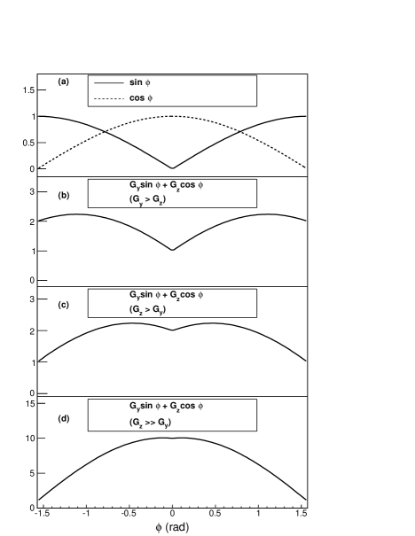
Figure 3: Schematic representation of the particle distribution, arising from the Cooper-Frye formula. The distribution is centered around the direction of motion ($\phi=0$) of the parton that deposits the energy momentum in the medium. Since the distribution is a sum of a $\sin(\phi)$ and a $\cos(\phi)$, its shape depends on the relative strength of their respective coefficients, $G_{y}$ and $G_{z}$. We show first the (a) $\sin(\phi)$ and $\cos(\phi)$ functions, (b) the case where $G_{y}>G_{z}$, (c) the case where $G_{z}>G_{y}$, and finally (d) the case where $G_{z}\gg G_{y}$.

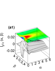
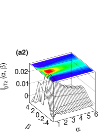
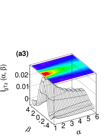
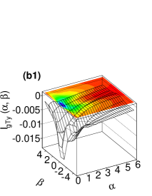
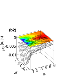
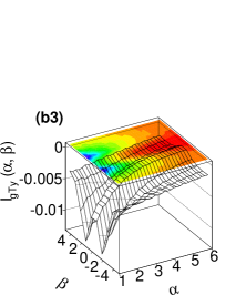
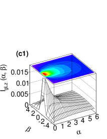
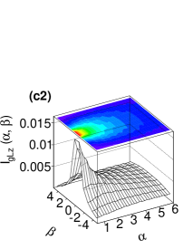
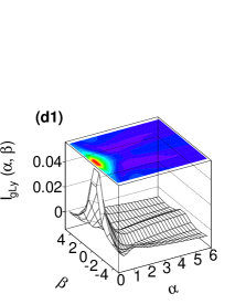
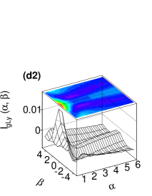
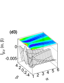
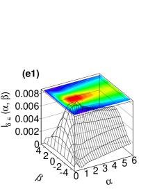
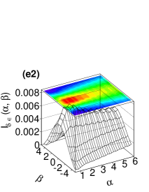
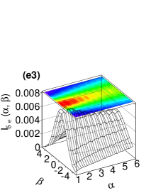
Figure 4: (Color on line) Three-dimensional plots and the corresponding contour plots for (a) $I_{g_{Tz}}$, (b) $I_{g_{Ty}}$, (c) $I_{g_{Lz}}$, (d) $I_{g_{Ly}}$ and (e) $I_{g_{\delta\epsilon}}$ defined in Eqs. (40), (41), (47), (48), and (49) as functions of $\alpha$ and $\beta$. The plots are shown from a minimum values of (1) $\alpha_{\mbox{\tiny{min}}}=0.1$ , (2) $\alpha_{\mbox{\tiny{min}}}=0.5$ and (3) $\alpha_{\mbox{\tiny{min}}}=1$ up to a maximum value of $\alpha_{\mbox{\tiny{max}}}=6$.

where $\phi$ is the angle that the momentum vector ${\mathbf{p}}$ makes with the $\hat{z}$ axis. We use Bjorken’s geometry; thus,

$$d^{3}p = p_{T}dp_{T}d\phi dp_{x},$$

$$p_{x} = p_{T}\sinh y,$$

$$dp_{x} = p_{T}\cosh y\ dy,$$

$$E = p_{T}\cosh y,$$ (4)

and therefore

$$E\frac{dN}{d^{3}p}=\frac{1}{p_{T}dp_{T}}\frac{dN}{d\phi dy}.$$ (5)

For simplicity we consider a freeze-out hypersurface of constant time,

$$d\Sigma_{\mu}=(d^{3}r,0,0,0).$$ (6)

Therefore, using Eqs. (1) and (5), the particle azimuthal distribution around the direction of motion of a fast moving parton within the $p_{T}$ interval $p_{T}^{\mbox{\tiny{min}}}\leq p_{T}\leq p_{T}^{\mbox{\tiny{miax}}}$ is given by

$$\left.\frac{dN}{dy}\right|_{y\simeq 0} = \frac{\Delta\tau\Delta y}{(2\pi)^{3}}\int_{p_{T}^{\mbox{\tiny{min}}}}^{p_{T}^{\mbox{\tiny{max}}}}dp_{T}p_{T}^{2}$$ (7)

$$\times \int d^{2}r[f(p\cdot u)-f(p_{0})],$$

with $\Delta\tau$ the freeze-out time interval and where we have assumed a perfect correlation between the space-time rapidity $\eta$ and $y$ to substitute $\Delta\eta$ by $\Delta y$. We assume that the equilibrium distribution is of the Boltzmann type. In this way, we have

$$f(p_{0}) = \exp[p_{T}/T_{0}]$$

$$f(p\cdot u) = \exp\left[\frac{p_{T}}{(T_{0}+\delta T)}\left(1-\frac{{\mathbf{g}}_{y}\sin\phi+{\mathbf{g}}_{z}\cos\phi}{\epsilon_{0}(1+c_{s}^{2})}\right)\right],$$

where $T_{0}$ is the background medium’s temperature and $\delta T$ is the change in temperature caused by the passing of the fast parton. Assuming that the energy density and temperature are related through Boltzmann’s law

$$\epsilon\propto T^{4},$$ (9)

one gets

$$\frac{\delta T}{T_{0}}=\frac{\delta\epsilon}{4\epsilon_{0}}.$$ (10)

Since for the validity of linearized hydrodynamics, both $\delta\epsilon$ and ${\mathbf{g}}$ need to be small quantities compared to $\epsilon_{0}$, we can expand the difference $f(p\cdot u)-f(p_{0})$ to linear order. Using Eqs. (LABEL:distexpl) and (10) we get

$$f(p\cdot u)-f(p_{0}) \simeq \left(\frac{p_{T}}{T_{0}}\right)\exp\left[-p_{T}/T_{0}\right]$$ (11)

$$\times \left(\frac{\delta\epsilon}{4\epsilon_{0}}+\frac{{\mathbf{g}}_{y}\sin\phi+{\mathbf{g}}_{z}\cos\phi}{\epsilon_{0}(1+c_{s}^{2})}\right),$$

Therefore, the particle azimuthal distribution around the direction of motion of a fast moving parton is given, in the linear approximation, by

$$\left.\frac{dN}{dy}\right|_{y\simeq 0} = \frac{\Delta\tau\Delta y}{(2\pi)^{3}}\int_{p_{T}^{\mbox{\tiny{min}}}}^{p_{T}^{\mbox{\tiny{max}}}}dp_{T}\frac{p_{T}^{3}}{T_{0}}\exp\left[-p_{T}/T_{0}\right]$$ (12)

$$\times \int d^{2}r\left(\frac{\delta\epsilon}{4\epsilon_{0}}+\frac{{\mathbf{g}}_{y}\sin\phi+{\mathbf{g}}_{z}\cos\phi}{\epsilon_{0}(1+c_{s}^{2})}\right).$$

Notice that the shape of the distribution around the direction of the fast moving parton depends on the quantities

$$G_{y} \equiv \int d^{2}r{\mathbf{g}}_{y},$$

$$G_{z} \equiv \int d^{2}r{\mathbf{g}}_{z}.$$ (13)

When $G_{y}>G_{z}$ the distribution is dominated by the $\sin\phi$ factor, giving rise to two peaks away from $\phi=0$. However, when $G_{z}>G_{y}$ the opposite happens and the distribution is dominated by the $\cos\phi$ factor with the two peaks close to $\phi=0$. These peaks become a single peak in the extreme case where $G_{z}\gg G_{y}$. This is illustrated in Fig. 3.

We now proceed to show that when the velocity of the moving parton is larger than the speed of sound, $G_{y}$ is mostly made out of longitudinal (sound) modes, whereas $G_{z}$ is mostly made out of wake (transverse) modes and that the latter dominates the former, giving rise to a particle distribution centered around the direction of motion of the moving parton.

III Linear viscous hydrodynamics

To compute the $g_{y}$ and $g_{z}$ components of the momentum density vector ${\mathbf{g}}$ which is deposited into the medium by the fast moving parton, we resort to using linearized viscous hydrodynamics. Assuming that the disturbance introduced by the parton is small, the medium’s energy momentum tensor can be written as

$$\Theta^{\mu\nu}=\Theta_{0}^{\mu\nu}+\delta\Theta^{\mu\nu},$$ (14)

where $\delta\Theta^{\mu\nu}$ is the perturbation generated by the parton and $\Theta_{0}^{\mu\nu}$ is the equilibrium energy momentum tensor of the underlying medium. Therefore, each of these components satisfies the equations

$$\partial_{\mu}\delta\Theta^{\mu\nu} = J^{\nu},$$

$$\partial_{\mu}\Theta_{0}^{\mu\nu} = 0,$$ (15)

where $J^{\nu}$ represents the source of the disturbance, which in this case corresponds to the fast moving parton. Here we consider that the parton can be represented by a localized disturbance of the form

$$J^{\nu}({\mathbf{x}},t)=\left(\frac{dE}{dx}\right)v^{\nu}\delta({\mathbf{x}}-{\mathbf{v}}t),$$ (16)

where $\left(dE/dx\right)$ is the energy loss per unit length and

$$v^{\nu}=(1,{\mathbf{v}}),$$ (17)

Effects of a finite source structure were studied in Ref. Neufeld1 , where it is found that differences in the energy density deposition between a finite extent source and a localized one exist only close to the source. Because a hydrodynamic description is anyway valid only for large distances from the source, compared to the transport mean free path, here we consider that the description of a source as localized exactly at the position of the fast parton; suffices.

Furthermore, we consider that the partons produced in the hard scattering are propagating asymptotically, that is, we ignore any finite time effects associated with the initial hard scattering during the collision. The latte have been raised and examined in a different context for example in Ref. Gossiaux . Although these effects are important and may very well be significant for the description of the energy loss of a fast moving parton in finite size media in this work our focus is on the time dependence associated with energy momentum deposited after the hard partons are produced, that is, while traveling into the medium, and on how the shape of the away side can be understood in terms of the energy deposited by two partons instead of one parton.

To describe the propagation of the disturbance caused by the source, Eqs. (15) are solved by considering that the energy momentum tensor $\Theta^{\mu\nu}$ consists of a piece that describes an isotropic fluid,

$$\Theta_{0}^{\mu\nu}=-pg^{\mu\nu}+(\epsilon+p)u_{0}^{\mu}u_{0}^{\nu}$$ (18)

and a disturbance $\delta\Theta^{\mu\nu}$ caused by the source, whose explicit components to first order in shear ($\eta$) and bulk ($\zeta$) viscosity are given by

$$\delta\Theta^{00} = \delta\epsilon,$$

$$\delta\Theta^{0i} = {\mathbf{g}},$$

$$\delta\Theta^{ij} = \delta_{ij}c_{s}^{2}\delta\epsilon-\frac{3}{4}\Gamma_{s}(\partial^{i}\mathbf{g}^{j}+\partial^{j}\mathbf{g}^{i}-\frac{2}{3}\delta_{ij}\nabla\cdot{\mathbf{g}})$$ (19)

$$- \zeta~{}\delta_{ij}\nabla\cdot{\mathbf{g}},$$

where $\epsilon(t,\mathbf{x})=\epsilon_{0}+\delta\epsilon(t,\mathbf{x})$ with $\epsilon_{0}$ correspond to the energy density of the background fluid, $\delta\epsilon$ corresponds to the energy density associated to the disturbance, and

$$\Gamma_{s}\equiv\frac{4\eta}{3\epsilon_{0}(1+c_{s}^{2})}$$ (20)

is the sound attenuation length.

In the linear approximation and vanishing bulk viscosity Neufeld1 , the dynamic description of the propagation of the disturbance is given by the first of Eqs. (15), whose explicit components can be written as

$$\partial_{0}\delta\epsilon+\nabla\cdot\mathbf{g} = J^{0},$$

$$\partial_{0}{\bf g}^{i}+\partial_{j}\delta\Theta^{ij} = J^{i}.$$ (21)

These equations can be readily solved in momentum space. We define the Fourier transform pair $f({\mathbf{x}},t)$ and $f({\mathbf{k}},\omega)$ as

$$f({\mathbf{x}},t)=\frac{1}{(2\pi)^{4}}\int d^{3}k\int d\omega\,e^{i{\bf k}\cdot{\bf x}-i\omega t}f({\mathbf{k}},\omega).$$ (22)

Using Eq. (22) in Eqs. (III), together with Eqs. (III), we obtain

$$-i\omega\delta\epsilon+i\mathbf{k}\cdot\mathbf{g} = J^{0},$$

$$-i\omega\mathbf{g}^{i}+ic_{s}^{2}k^{i}\delta\epsilon+\frac{3}{4}\Gamma_{s}[k^{2}\mathbf{g}^{i}+\frac{k^{i}}{3}(\mathbf{k}\cdot\mathbf{g})] = J^{i}.$$ (23)

Thus the perturbed energy density, $\delta\epsilon$ and momentum density components ${\bf g}^{i}$, can be obtained by solving the algebraic system of Eqs. (III), and the solutions are given by Neufeld2

$$\delta\epsilon({\mathbf{k}},\omega) = \frac{i{\mathbf{k}}\cdot{\mathbf{J}}({\mathbf{k}},\omega)+J^{0}({\mathbf{k}},\omega)(i\omega-\Gamma_{s}k^{2})}{\omega^{2}-c_{s}^{2}k^{2}+i\Gamma_{s}\omega k^{2}},$$ (24)

$${\mathbf{g}}_{L}({\mathbf{k}},\omega) = \frac{i\left[\frac{\omega}{k^{2}}{\mathbf{k}}\cdot{\mathbf{J}}({\mathbf{k}},\omega)+c_{s}^{2}J^{0}({\mathbf{k}},\omega)\right]{\mathbf{k}}}{\omega^{2}-c_{s}^{2}k^{2}+i\Gamma_{s}\omega k^{2}},$$ (25)

$${\bf g}_{T}({\mathbf{k}},\omega) = {\bf g}-{\bf g}_{L}=\frac{i{\mathbf{J}}_{T}({\mathbf{k}},\omega)}{\omega+i\frac{3}{4}\Gamma_{s}k^{2}},$$ (26)

where we have written the momentum density vector in terms of its transverse and longitudinal components with respect to the Fourier mode $\mathbf{{k}}$, namely,

$${\mathbf{g}}={\mathbf{g}}_{L}+{\mathbf{g}}_{T},$$ (27)

with the definition of longitudinal and transverse components of any vector ${\sigma}$ given by

$$\mbox{\boldmath${\sigma}$}_{L} \equiv \frac{(\mbox{\boldmath${\sigma}$}\cdot{\mathbf{k}})}{k^{2}}{\mathbf{k}},$$

$$\mbox{\boldmath${\sigma}$}_{T} \equiv \mbox{\boldmath${\sigma}$}-\mbox{\boldmath${\sigma}$}_{L}.$$ (28)

Note that the source term $J^{\nu}$ in Eq. (16) is Fourier transformed to

$$J^{\nu}({\bf k},\omega)=(2\pi)\left(\frac{dE}{dx}\right)\delta({\bf k\cdot v}-\omega)v^{\nu},$$ (29)

where we assumede a constant energy loss per unit length.

From Eqs. (24)–(26) one can obtain the space-time solutions for $\delta\epsilon({\mathbf{x}},t)$ and ${\mathbf{g}}({\mathbf{x}},t)$ upon use of Eq. (22). The corresponding expressions are

$${\bf g}_{T}({\bf x},t) = i(2\pi)\left(\frac{dE}{dx}\right)\int\frac{d^{3}k}{(2\pi)^{3}}\int\frac{d\omega}{(2\pi)}e^{i{\bf k}\cdot{\bf x}-i\omega t}$$ (30)

$$\times \left[{\bf v}-\frac{({\bf k\cdot J}){\bf k}}{k^{2}}\right]\frac{\delta({\bf k}\cdot{\bf v}-\omega)}{\omega+i\frac{3}{4}\Gamma_{s}k^{2}}$$

$${\bf g}_{L}({\bf x},t) = i(2\pi)\left(\frac{dE}{dx}\right)\int\frac{d^{3}k}{(2\pi)^{3}}\int\frac{d\omega}{(2\pi)}e^{i{\bf k}\cdot{\bf x}-i\omega t}$$ (31)

$$\times {\bf k}\left[\frac{\omega}{k^{2}}{\bf k}\cdot{\bf v}+c_{s}^{2}\right]\frac{\delta({\bf k}\cdot{\bf v}-\omega)}{\omega^{2}-c_{s}^{2}k^{2}+i\Gamma_{s}\omega k^{2}}$$

and

$$\delta\epsilon({\bf x},t) = i(2\pi)\left(\frac{dE}{dx}\right)\int\frac{d^{3}k}{(2\pi)^{3}}\int\frac{d\omega}{(2\pi)}e^{i{\bf k}\cdot{\bf x}-i\omega t}$$

$$\times \left[i{\bf k}\cdot{\bf v}+i\omega-\Gamma_{s}k^{2}\right]\frac{\delta({\bf k}\cdot{\bf v}-\omega)}{\omega^{2}-c_{s}^{2}k^{2}+i\Gamma_{s}\omega k^{2}}.$$

To compute the integrals in Eqs. (30)–(LABEL:deltaepsilon(x)) we use cylindrical coordinates with the $k_{z}$ direction along the direction of motion, ${\mathbf{v}}$, of the fast parton. It is easier to start with the components of ${\bf g}_{T}$. After carrying out the frequency and angular integration, we get for the $z$ component

$$\left({\bf g}_{T}\right)_{z} = i(2\pi)\left(\frac{dE}{dx}\right)v\int_{0}^{\infty}\frac{dk_{T}}{(2\pi)^{2}}\int_{-\infty}^{\infty}\frac{dk_{z}}{(2\pi)}e^{ik_{z}(z-vt)}$$ (33)

$$\times \frac{k_{T}^{3}{\mbox{J}}_{0}(k_{T}x_{T})}{(k_{z}^{2}+k_{T}^{2})[vk_{z}+i\frac{3}{4}\Gamma_{s}(k_{z}^{2}+k_{T}^{2})]},$$

where ${\mbox{J}}_{0}$ is a Bessel function and $x_{T}=\sqrt{y^{2}}$ is the distance from the parton along the transverse direction (along the $\hat{y}$ axis in the geometry we are using). The integration over $k_{z}$ is performed using contour integration. For causal motion ($z-vt>0$) we close the contour on the lower half $k_{z}$-plane. The poles that contribute are located at

$$k_{z}=\left\{\begin{array}[]{c}-ik_{T},\\ i\frac{2v}{3\Gamma_{s}}\left(1-\sqrt{1+\left(\frac{3\Gamma_{s}k_{T}}{2v}\right)^{2}}\right).\end{array}\right.$$ (36)

After carrying out the $k_{z}$ integration, the remaining integral can be expressed in terms of the dimensionless quantities

$$\xi \equiv \left(\frac{3\Gamma_{s}}{2v}\right)k_{T},$$

$$\alpha \equiv |z-vt|/\left(\frac{3\Gamma_{s}}{2v}\right),$$

$$\beta \equiv x_{T}/\left(\frac{3\Gamma_{s}}{2v}\right),$$ (37)

as

$$\left({\bf g}_{T}\right)_{z} = -\left(\frac{1}{4\pi}\right)\left(\frac{dE}{dx}\right)\left(\frac{2v}{3\Gamma_{s}}\right)^{2}\int_{0}^{\infty}d\xi\ \xi{\mbox{J}}_{0}(\xi\beta)$$ (38)

$$\times \left[e^{-\alpha\xi}+\frac{e^{-\alpha(\sqrt{1+\xi^{2}}-1)}}{[\sqrt{1+\xi^{2}}-(1+\xi^{2})]}\right].$$

Notice that although the source term describes infinite propagation, in practice the initial and final times of the evolution are implemented by considering a finite interval for the variable $\alpha$, which represents the distance to the source in units of the sound attenuation length.

The first term in Eq. (38) can be analytically integrated. For numerical purposes, it is more convenient to rewrite the second term after the change of variable:

$$s=\sqrt{1+\xi^{2}}-1.$$ (39)

The final result is

$$\left({\bf g}_{T}\right)_{z} = \left(\frac{1}{4\pi}\right)\left(\frac{dE}{dx}\right)\left(\frac{2v}{3\Gamma_{s}}\right)^{2}\left[-\frac{\alpha}{\left(\alpha^{2}+\beta^{2}\right)^{\frac{3}{2}}}\right.$$ (40)

$$+ \left.\int_{0}^{\infty}ds(s+2){\mbox{J}}_{0}\left(\beta\sqrt{s(s+2)}\right)e^{-\alpha s}\right]$$

$$\equiv \left(\frac{1}{4\pi}\right)\left(\frac{dE}{dx}\right)\left(\frac{2v}{3\Gamma_{s}}\right)^{2}I_{g_{Tz}}(\alpha,\beta).$$

In a similar fashion we get

$$\left({\bf g}_{T}\right)_{y} = \left(\frac{1}{4\pi}\right)\left(\frac{dE}{dx}\right)\left(\frac{2v}{3\Gamma_{s}}\right)^{2}\left[\frac{\beta}{\left(\alpha^{2}+\beta^{2}\right)^{\frac{3}{2}}}\right.$$ (41)

$$- \left.\int_{0}^{\infty}ds\sqrt{s(s+2)}{\mbox{J}}_{1}\left(\beta\sqrt{s(s+2)}\right)e^{-\alpha s}\right]$$

$$\equiv \left(\frac{1}{4\pi}\right)\left(\frac{dE}{dx}\right)\left(\frac{2v}{3\Gamma_{s}}\right)^{2}I_{g_{Ty}}(\alpha,\beta).$$

The computation of the components of ${\mathbf{g}}_{L}$ is more involved due to the analytic structure of the poles in the complex $k_{z}$-plane. Let us fist compute the $z$ component. After carrying out the frequency and angular integration we get

$$\left({\bf g}_{L}\right)_{z} = i(2\pi)\left(\frac{dE}{dx}\right)\int_{0}^{\infty}\frac{dk_{T}}{(2\pi)^{2}}\int_{-\infty}^{\infty}\frac{dk_{z}}{(2\pi)}e^{ik_{z}(z-vt)}$$ (42)

$$\times \frac{k_{T}{\mbox{J}}_{0}(k_{T}x_{T})k_{z}[k_{z}^{2}+\frac{c_{s}^{2}}{v^{2}}(k_{z}^{2}+k_{T}^{2})]}{(k_{z}^{2}+k_{T}^{2})[k_{z}^{2}+(i\frac{\Gamma_{s}}{v}k_{z}-\frac{c_{s}^{2}}{v^{2}})(k_{z}^{2}+k_{T}^{2})]}.$$

Notice that the integrand contains the parameter $c_{s}^{2}/v^{2}$ and that for a fast moving parton $v\simeq 1$.

This allows for an approximation to be implemented in order to render the results more transparent: We consider the parameter $c_{s}^{2}/v^{2}<1$ to be small such that we can expand the integrands before calculating the remaining integral. This approximation is sustained by lattice estimates (see, for instance, Ref. Borsanyi ) of the speed of sound which show that $c_{s}$ increases monotonically from about one-third of the ideal gas limit ($\simeq\sqrt{1/3}$) for $T\gtrsim 1.5T_{c}$ and approaches this limit only for $T>4T_{c}$, where $T_{c}$ is the critical temperature for the phase transition. Therefore, even though the approximation $c_{s}^{2}/v^{2}<1$ could only be regarded as a parametric limit, the fact that for experimental conditions $c_{s}^{2}<1/3$ makes the approximation to be a good one for the present context. Here we use $c_{s}^{2}=1/3$, which can then be taken as a worst-case scenario for a numerical estimate. Thus, for conditions close to the ones after a heavy-ion reaction $c_{s}^{2}/v^{2}<1$ and we can expand the integrand in Eq. (42) in this parameter. Notice that in the literature there are different approximation schemes to carry out the integrals such as the ones in Eq. (42). For instance, in order to calculate the energy momentum deposited by longitudinal modes, the approximation $s^{2}/\Gamma_{s}\gg k_{T}$ is made in Refs. Neufeld3 and Neufeld4 , which allows to integrate over $k_{z}$ analytically, before proceeding to the numerical computation of the integral over $k_{T}$.

Therefore, to first order in $c_{s}^{2}/v^{2}$, we get

$$\left({\bf g}_{L}\right)_{z} = i(2\pi)\left(\frac{dE}{dx}\right)\int_{0}^{\infty}\frac{dk_{T}}{(2\pi)^{2}}k_{T}{\mbox{J}}_{0}(k_{T}x_{T})$$

$$\int_{-\infty}^{\infty}\frac{dk_{z}}{(2\pi)}$$

$$\times \left\{\frac{k_{z}^{2}e^{ik_{z}(z-vt)}}{(k_{z}^{2}+k_{T}^{2})[k_{z}+(i\frac{\Gamma_{s}}{v})(k_{z}^{2}+k_{T}^{2})]}\right.$$

$$+ \left.\left(\frac{c_{s}^{2}}{v^{2}}\right)\frac{2k_{z}(i\frac{\Gamma_{s}}{v})(k_{z}^{2}+k_{T}^{2})e^{ik_{z}(z-vt)}}{[k_{z}+(i\frac{\Gamma_{s}}{v})(k_{z}^{2}+k_{T}^{2})]}\right\}.$$

For causal motion ($z-vt>0$) we close the contour on the lower half $k_{z}$-plane. The poles that contribute are located at

$$k_{z}=\left\{\begin{array}[]{c}-ik_{T},\\ i\frac{v}{2\Gamma_{s}}\left(1-\sqrt{1+\left(\frac{2\Gamma_{s}k_{T}}{v}\right)^{2}}\right).\end{array}\right.$$ (46)

The remaining integral over $k_{T}$ can be expressed in terms of the dimensionless quantities defined in Eq. (37). For numerical purposes, it is more convenient to rewrite this integral after the change of variable in Eq. (39). The result reads as follows:

$$\left({\bf g}_{L}\right)_{z} = \left(\frac{1}{4\pi}\right)\left(\frac{dE}{dx}\right)\left(\frac{2v}{3\Gamma_{s}}\right)^{2}\left[\frac{\alpha}{\left(\alpha^{2}+\beta^{2}\right)^{\frac{3}{2}}}\right.$$ (47)

$$- \frac{9}{16}\int_{0}^{\infty}ds{\mbox{J}}_{0}\left(\frac{3}{4}\beta\sqrt{s(s+2)}\right)e^{-\frac{3}{4}\alpha s}\left(s\right.$$

$$+ \left.\left.c_{s}^{2}/v^{2}\left(\frac{3\alpha s}{2(s+1)}-\frac{2}{(s+1)^{2}}-2\right)\right)\right]$$

$$\equiv \left(\frac{1}{4\pi}\right)\left(\frac{dE}{dx}\right)\left(\frac{2v}{3\Gamma_{s}}\right)^{2}I_{g_{Lz}}(\alpha,\beta).$$

In a similar fashion we obtain

$$\left({\bf g}_{L}\right)_{y} = \left(\frac{1}{4\pi}\right)\left(\frac{dE}{dx}\right)\left(\frac{2v}{3\Gamma_{s}}\right)^{2}\left[\frac{\beta}{\left(\alpha^{2}+\beta^{2}\right)^{\frac{3}{2}}}\right.$$ (48)

$$+ \frac{9}{16}\int_{0}^{\infty}ds{\mbox{J}}_{1}\left(\frac{3}{4}\beta\sqrt{s(s+2)}\right)e^{-\frac{3}{4}\alpha s}\left(-1\right.$$

$$+ \left.\left.c_{s}^{2}/v^{2}\left(\frac{2}{(s+1)^{2}}-\frac{3\alpha}{2(s+1)}-\frac{2}{s}\right)\right)\right]$$

$$\equiv \left(\frac{1}{4\pi}\right)\left(\frac{dE}{dx}\right)\left(\frac{2v}{3\Gamma_{s}}\right)^{2}I_{g_{Ly}}(\alpha,\beta),$$

and

$$\delta\epsilon = \left(\frac{1}{4\pi}\right)\left(\frac{dE}{dx}\right)\left(\frac{2v}{3\Gamma_{s}}\right)^{2}\left(\frac{9}{8v}\right)$$ (49)

$$\times \int_{0}^{\infty}ds{\mbox{J}}_{0}\left(\frac{3}{4}\beta\sqrt{s(s+2)}\right)e^{-\frac{3}{4}\alpha s}$$

$$\times \left[1+\frac{2c_{s}^{2}/v^{2}}{s}\left(-1+\frac{1+s\left(3+s+\frac{3}{4}\alpha(s+1)\right)}{(s+1)^{2}}\right)\right]$$

$$\equiv \left(\frac{1}{4\pi}\right)\left(\frac{dE}{dx}\right)\left(\frac{2v}{3\Gamma_{s}}\right)^{2}\left(\frac{9}{8v}\right)I_{\delta\epsilon}(\alpha,\beta).$$

Figure 4 shows three-dimensional plots of $I_{g_{Tz}},I_{g_{Ty}},I_{g_{Lz}},I_{g_{Ly}}$ and $I_{g_{\delta\epsilon}}$ as functions of $\alpha$ and $\beta$. Shown also are the corresponding contour plots. To test the sensitivity of the results on the distance to the source, the plots are shown starting from a minimum value of $\alpha_{\mbox{\tiny{min}}}=0.1,0.5,1$ up to a maximum value of $\alpha_{\mbox{\tiny{max}}}=6$. Figure 5 shows the integrals of the above functions over the domain $\alpha_{\mbox{\tiny{min}}}<\alpha<\alpha_{\mbox{\tiny{max}}}$, $-5<\beta<5$ for the different values of $\alpha_{\mbox{\tiny{min}}}$. Shown also are the values of the combinations $I_{z}\equiv I_{g_{Tz}}+I_{g_{Lz}}$ and $I_{y}\equiv I_{g_{Ty}}+I_{g_{Ly}}$. Notice that, for all of the shown values of $\alpha_{\mbox{\tiny{min}}}$, the largest contribution to $I_{z}$ comes from $I_{g_{Tz}}$, which is the wake or transverse mode, whereas the largest contribution to $I_{y}$ comes from $I_{g_{Ly}}$, which is the sound or longitudinal mode. Moreover, $I_{z}$ is always larger than $I_{y}$. This last result shows that for the case treated here, where $c_{s}^{2}/v^{2}<1$, the momentum deposition is preferentially forward peaked.

IV Azimuthal correlations

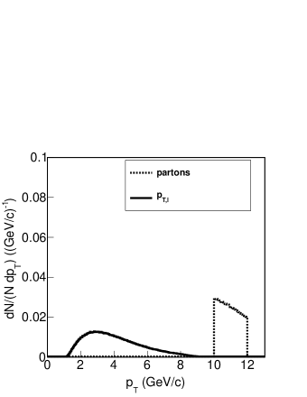
Figure 7: Hadron momentum distribution obtained from a leading parton with momentum in the range 10 GeV $\leq p_{T}\leq$ 12 GeV.

We now proceed to use the formalism developed above to compute the azimuthal angular correlations for events where the leading hadron has a momentum larger than or equal to the associated ones. Figure 6 shows the per-trigger correlations for the cases where the leading hadron is produced in a momentum range 3 GeV $\leq p_{T}\leq$ 4 GeV and the associated ones in the momentum ranges 0.4 GeV $\leq p_{T}\leq$ 1 GeV, 1 GeV $\leq p_{T}\leq$ 2 GeV, 2 GeV $\leq p_{T}\leq$ 3 GeV and 3 GeV $\leq p_{T}\leq$ 4 GeV, compared to data from PHENIX PHENIX . To obtain these correlations we have generated $2\to 3$ hard scattering parton events using the MadGraph5 event generator madgraph , within the momentum window 10 GeV $\leq p_{T}\leq$ 12 GeV. Out of the three partons, we choose the one with the largest momentum to become the leading hadron by collinear fragmentation using the Kniehl, Kramer and Pötter (KKP) parton fragmentation functions KKP . The other two partons in the event travel within the medium and thus represent the sources of energy momentum deposition in the away side. We consider that these partons travel 6 fm on average Ayala1 , with a medium-induced energy loss per unit length $dE/dx=$ 2 GeV/fm. Therefore, on average, these partons transfer all of their initial momentum to the medium. For these away side partons, we compute the angular distribution around their direction of motion by means of the Cooper-Frye and linear viscous hydrodynamics formalisms, described in Secs. II and III. We use the value $\alpha_{\mbox{\tiny{min}}}=0.1$. Since we consider massless partons, we take their speed to be $v=0.9995c$. The sound attenuation length is taken to be $\Gamma_{s}=1/(3\pi T_{0})$, which results from taking $\eta=1/(4\pi)$ and considering the value $T_{0}=350$ MeV, and the sound velocity is $c_{s}=1/\sqrt{3}$. To produce final-state hadrons out of the away side partons that emerge via the Cooper-Frye formula, we consider that the partons in the head shock region carry half of the hard-scattering parton momentum. We subsequently let these partons produce final-state hadrons using once again the KKP in vacuum fragmentation functions. This procedure is intended to mimic surface emission of the leading parton together with in-medium energy momentum deposited by the away side ones. The distributions thus obtained are multiplied by the same correction factor, $f\approx 30$. This factor is introduced for data comparison purposes and has to be regarded as a quantitative measure of the dynamical details left out in this analysis. However, we emphasize that this factor is the same for all bins shown. The hadron momentum distributions obtained from the leading and associate partons are shown in Figs. 7 and 8, respectively.

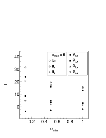
Figure 5: Integrals of the functions $I_{g_{Tz}},I_{g_{Ty}},I_{g_{Lz}},I_{g_{Ly}}$ and $I_{g_{\delta\epsilon}}$ over the domain $\alpha_{\mbox{\tiny{min}}}<\alpha<\alpha_{\mbox{\tiny{max}}}$, $-5<\beta<5$ for the different values of $\alpha_{\mbox{\tiny{min}}}$. We also plot the values of the combinations $I_{z}\equiv I_{g_{Tz}}+I_{g_{Lz}}$ and $I_{y}\equiv I_{g_{Ty}}+I_{g_{Ly}}$. Notice that, for all of values of $\alpha_{\mbox{\tiny{min}}}$, the largest contribution to $I_{z}$ comes from $I_{g_{Tz}}$, which is the wake or transverse mode, whereas the largest contribution to $I_{y}$ comes from $I_{g_{Ly}}$, which is the sound or longitudinal mode. Moreover, $I_{z}$ is always larger than $I_{y}$.

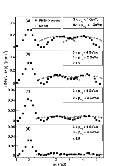
Figure 6: Per-trigger azimuthal angular correlations. Shown are four different cases, each one having the leading hadron produced with a fixed momentum range 3 GeV $\leq p_{T}\leq$ 4 GeV. The associated hadrons are in following the momentum ranges: (a) 0.4 GeV $\leq p_{T}\leq$ 1 GeV, (b) 1 GeV $\leq p_{T}\leq$ 2 GeV, (c) 2 GeV $\leq p_{T}\leq$ 3 GeV and (d) 3 GeV $\leq p_{T}\leq$ 4 GeV. The theoretical distributions are multiplied by the same correction factor, $f\approx 30$. The results are compared to data from PHENIX PHENIX .

Notice that Fig. 6 shows a quite good agreement of this simple scenario with the correlation data, particularly because it reproduces the systematics of double-hump decreasing intensity as the momentum of the away side hadrons becomes closer to the momentum of the leading hadron.

V Summary and conclusions

In this work, we have studied the way that fast moving partons deposit their energy momentum when traveling in a medium. We showed that, for conditions resembling a medium produced in a heavy-ion reaction, energy momentum is preferentially deposited along the head shock and that, in order to produce a double-hump structure in the away side of azimuthal correlations, one can consider that two partons, instead of one, travel towards the away side. We argued that these away side partons can be originally produced by a $2\to 3$ hard scattering. Even though $2\to 3$ parton processes are suppressed with respect to $2\to 2$ ones by an extra power of $\alpha_{s}$, there is also a kinematic enhancement that, partially compensates. This is due to the fact that for a given energy deposited in the away side, the partons from $2\to 3$ processes are produced with lower momentum than the away side parton in $2\to 2$ processes; thus, the former are more copiously produced.

We resorted to linear viscous hydrodynamics to compute the medium response to the fast moving partons and the Cooper-Frye formula to compute the parton distribution originated from this disturbance in a static background medium. To mimic a scenario where the leading hadron comes from surface emission and the away side partons deposit all of their original energy momentum within the medium, we selected partons produced in $2\to 3$ processes, evolving the parton with the highest energy to become the leading hadron using KKP in vacuum fragmentation. Also, the head shock region around the direction of motion of the away side partons, is assumed to carry half of the original hard-scattering parton momentum. The partons in the head shock region are then hadronized using also KKP in vacuum fragmentation. The comparison to PHENIX data shows that this simple scenario reproduces the systematics of a decreasing away side correlation when the momentum of the associated hadrons becomes closer to the momentum of the leading hadron. This scenario seems to avoid the shortcomings of the Mach cone as the origin of the double-hump structure in the away side.

Notice that another possibility to have three partons in the final state is to start from a $2\to 2$ process followed by a large angle parton emission. The probability of this process, however, is suppressed with respect to (direct) $2\to 3$ processes. To see this, consider a given total momentum for the two away side partons. If these come from a single parton in the away side, which then radiates a parton with a large angle, the radiating parton needs to be produced with a momentum of the order of twice the momentum of each of the two final away side partons. This is to say that, in order for the radiated and the radiating partons to have their momenta add up to the momentum of the leading parton, the radiating (original) parton needs to have a momentum of order twice the momentum of what it will have after radiating. Therefore, we come back to the phase space suppression argument we have put forward, namely that producing a parton with a larger momentum has less phase space than producing partons with lesser momenta. If we now account for the extra power of $\alpha_{s}$, these kinds of processes are suppressed with respect to (direct) $2\to 3$ processes.

We did not attempt to quantitatively address parton splitting in $2\to 2$ processes. However, recall that splitting is important in two situations: (1) the soft and collinear regions and (2) for the evolution of the parton shower that makes up the final-state jet. For the first case, collinear and soft divergences are taken care of by the dipole substraction implemented in MadGraph 5 that we use. On the other hand, real (as opposed to singular and thus virtually corrected) splitting needs to be accounted for when pursuing a more detailed analysis of the jet shapes and their possible in-medium modification. In this work, we adopted the simpler point of view that the energy momentum is deposited in the forward direction by the parton that plows through the medium and not by the other (lesser momentum) partons that this one may split into. In any case, we believe that splitting should be important for the shape of the individual jet but not for the double-hump structures in the away side, unless the splitting results in a large angle emission, in which case we come back to the discussion above. In this sense, splitting should not affect the qualitative description we presented.

The scenario we considered corresponds to the analog case of surface emission in $2\to 2$ processes, whereby the leading hadron comes from a parton emitted outwards from the surface and the away side hadron comes from a parton emitted towards the interior of the fireball. In the $2\to 3$ case, we consider the leading parton emitted radially outwards and the away side partons to travel within the fireball an average distance such that, for the energy loss per unit length we have taken, they deposit on average all their energy within the medium. A more realistic scenario should consider all the possibilities, that is, partons traveling towards the fireball produced with larger and lower energies and different directions. Some of these will not deposit all of their energy within the medium and could thus hadronize outside by fragmentation. The details of the calculation can certainly vary but it is clear that these last kinds of processes add up to the signal, albeit in a way that needs to be quantified. Since the purpose of the present work was to call attention for an alternative process to the usual Mach cone or the initial-state fluctuation scenarios, we did not carry out such detailed calculations. We are planning on doing so and reporting elsewhere shortly.

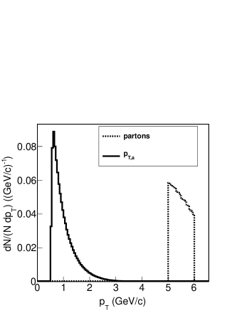
Figure 8: Hadron momentum distribution obtained from an associated parton with momentum in the range 5 GeV $\leq p_{T}\leq$ 6 GeV.

For the case where the background is not static, one could in principle consider different scenarios. Since the hard scattering happens at short times, the main effect should be caused by a dilution of the medium due to longitudinal expansion, given that transverse expansion sets in at larger times. This dilution in turn can be accounted for by a decreasing energy density of the background fluid, resulting in a larger sound attenuation length and therefore a smaller energy momentum deposition within the medium. The Cooper-Frye formula could no longer be implemented at a constant-time hypersurface and one would need to resort to a Bjorken-like scenario whereby freeze-out happens over a proper time period which can be related to a temperature interval. To quantitatively test the differences between a dynamic and a static scenario, we felt it was important first to have the latter as the reference to build on top of it with other effects, such as expansion. We are certainly planning to include these effects and report on the findings shortly after. A more detailed analysis is currently under way to explore the systematics of away side correlations for a larger set of conditions and will be reported elsewhere.

References

- (1) C. Adler et al. (STAR Collaboration), Phys. Rev. Lett. 90 082302 (2003).
- (2) A. Adate et al. (PHENIX Collaboration), Phys. Rev. C 78, 014901 (2008).
- (3) M. M. Aggarwal et al. (STAR Collaboration), Phys. Rev. C 82, 024912 (2010); A. Adare et al. (PHENIX Collaboration), Phys. Rev. Lett. 104, 252301 (2010).
- (4) J. Casalderrey-Solana, J. Phys. G 34, S345 (2007).
- (5) T. Renk and J. Ruppert, Phys. Rev. C 76, 014908 (2007).
- (6) J. Casalderrey-Solana, E. V. Shuryak and D. Teaney, PoS CFRNC2006, 022 (2006).
- (7) G. Torrieri, B. Betz, J. Noronha and M. Gyulassy, Acta Phys. Polon. B39, 3281 (2008).
- (8) I. Bouras, A. El, O. Fochler, H. Niemi, Z. Xu and C. Greiner, Phys. Lett. B 710, 641 (2012).
- (9) R. B. Neufeld and I. Vitev, Phys. Rev. C 86, 024905 (2012).
- (10) P. Sorensen (STAR Collaboration), J. Phys. G 38, 124029 (2011); K. Aamodt et al. (ALICE Collaboration), Phys. Rev. Lett. 107, 032301 (2011).
- (11) F. Wang (STAR Collaboration), arXiv:1201.5006; H. Agakishiev et al. (STAR Collaboration), arXiv:1010.0690.
- (12) A. Ayala, J. Jalilian-Marian, J. Magnin, A. Ortiz, G. Paić and M. E. Tejeda-Yeomans, Phys. Rev. Lett. 104, 042301 (2010); Phys. Rev. C 84, 024915 (2011).
- (13) A. Ayala, I. Dominguez, J. Jalilian-Marian, J. Magnin and M. E. Tejeda-Yeomans Phys. Rev. C 86, 034901 (2012).
- (14) F. Cooper and G. Frye, Phys. Rev. D 10, 186 (1974).
- (15) R. B. Neufeld, Phys. Rev. C 79, 054909 (2009).
- (16) R. B. Neufeld and T. Renk, Phys. Rev. C 82, 044903 (2010).
- (17) P.-B. Gossiaux, S. Peigne, C. Brandt and J. Aichelin, JHEP 0704, 012 (2007)
- (18) R. B. Neufeld, Phys. Rev. D 78, 085015 (2008).
- (19) Szabolcs Borsanyi, et al., JHEP 11, (2010) 077.
- (20) J. Alwall et al., JHEP 1106, 128 (2011).
- (21) B.A. Kniehl, G. Kreimer and B. Potter, Nucl. Phys. B 582, 514 (2000).