Abstract

To explore possibilities of avoiding coincidence problem in $f(R)$ gravity we consider models in Einstein conformal frame which are equivalent to Einstein gravity with a minimally coupled scalar field. As the conformal factor determines the coupling term and hence the interaction between matter and dark energy, the function $f(R)$ can in principle be determined by choosing an appropriate function for the deceleration parameter only. Possible behavior of $f(R)$ to avoid coincidence problem are investigated in two such cases.

Key Words: Cosmology; Dark energy; Coincidence Problem; $f(R)$ gravity.

1 Introduction

It is now more than a decade when the first observational evidence indicated that our Universe might have been expanding with acceleration[1]. With a growing number of data favoring such evidences over past few years such doubt has now turned into certainty that the Universe has entered an accelerated phase of expansion from a decelerated phase very recently[2][3]. This observational fact however needs a solid theoretical support which appears to be a major challenge in cosmology today. Efforts to resolve this matter have been made so far in two possible directions. One approach is to introduce a new term in the energy-momentum side of the Einstein’s equation which will act as a source of gravity with repulsive effect and initiate acceleration in the course of expansion. Such a source has been termed in literature as ‘Dark Energy’ due to its unknown nature. It is usually parameterized by an equation of state of the form $\omega_{DE}=p/\rho$. From Friedmann equation one can see that a value of $\omega_{DE}<-1/3$ is required for accelerated cosmic expansion. The most natural and simplest choice as a candidate for dark energy could have been the Cosmological Constant $\Lambda$ with equation of state $\omega_{DE}=-1$. But if one believes that vacuum energy is the origin of it then one fails to find any mechanism to obtain a value of $\Lambda$ that is 120 orders of magnitude less than the theoretical prediction to be consistent with observation. Attempts were made by introducing the concept of varying $\Lambda$ to explain observation but with same equation of state $\omega_{DE}=-1$[4]. Possibilities of evolving $\omega_{DE}$ were also explored in many dynamical dark energy models. Primary candidates in this category are scalar field models such as Quintessence[5] and K-essence[6]. A common example to quintessence is the energy of a slowly evolving scalar field that has not yet reached the minimum of its potential $V(\phi)$, similar to the inflaton field used to describe the inflationary phase of the Universe. In quintessence models the parameter range is $-1<\omega_{DE}<-1/3$, and the dark energy density decreases with a scale factor $a(t)$ as $\rho_{DE}\propto a^{-3(1+\omega_{DE})}$[7]. A specific exotic form of dark energy denoted phantom energy, with $\omega_{DE}<-1$, has also been proposed[8]. It possesses peculiar properties, such as the violation of the energy conditions and an infinitely increasing energy density. However, recent fits to supernovae, cosmic microwave background radiation (CMBR) and weak gravitational lensing data indicate that an evolving equation of state crossing the phantom divide, is mildly favored, and several models have been proposed in the literature[9]. In particular, models considering a redshift dependent equation of state, possibly provide better fits to the most recent and reliable SN Ia supernovae Gold dataset. A few comprehensive and recent review articles on dark energy may be of interest in this regard[10].

The alternative way to explain cosmic acceleration is to anticipate that large scale dynamics of the Universe is not governed by Einstein’s equations. In a classical generalization of general relativity, the Ricci scalar $R$ in Einstein-Hilbert action is replaced by a more general function $f(R)$ which modifies the geometry-side of the Einstein’s equation[11]. Earlier interest in $f(R)$ theories was motivated by inflationary scenarios as for instance, in the Starobinsky model[12]. Recently, a number of models in $f(R)$ modified theories of gravity has been verified in an attempt to explain the late-time accelerated expansion of the Universe. In particular, it has been shown that cosmic acceleration can indeed be explained in the context of $f(R)$ gravity[13], and the conditions of viable cosmological models have also been derived[14]. In the context of local tests in the Solar System regime, severe weak field constraints however, seem to rule out most of the models proposed so far[15], although viable models do exist[16]. Some recent reviews on $f(R)$ gravity may be of interest in this regard[17].

There exist many cosmological models in ‘modified gravity’ as well as ‘dark energy models’ that can successfully explain the observed late-time acceleration. However, there is no strong reason to choose one as better than the other. Not only that, there remain many unsolved issues related to all these approaches. One important issue among those is the Coincidence Problem[18]. If we accept that the observed acceleration is being caused by some ‘dark energy’ it is striking to find out that in our present Universe the density of dark energy and dark matter are of the same order. In fact any cosmological model successful in explaining late-time acceleration will necessarily suggest that dark energy density has started dominating over matter energy very recently. Now the question is why is it happening now? Is it a mere coincidence or is there some deep underlying reason behind it? This Coincidence Problem has been addressed in literature extensively[19]. One way to get rid of this is to design a model in which the ratio of matter density to dark energy density settles down with evolution to its present day value quickly and remains stationary for a long period until today so that the coincidence problem does not arise. However such a model needs interaction between dark energy and matter. Attempts to realize the coincidence problem as a consequence of interaction between matter sector and dark energy are not new[20]. The suggested interaction terms in all such attempts are however phenomenological and are not derived from any fundamental theory. In this present note we address the coincidence problem in the context of $f(R)$ gravity models in Einstein conformal frame. The conformally rescaled metric in such a model has a scalar field partner that act as another dynamical variable of the vacuum sector. Understandably this scalar field is not a kind of matter field and is actually given in terms of $f(R)$. There exists a coupling between this scalar degree of freedom and the matter sector induced by this conformal transformation and the interaction between matter and dark energy opens up the possibility of addressing the coincidence problem. The field equations look very much like those of quintessence models but with a difference. The interaction term is given by the conformal factor and hence the coupling constant is universal in a sense that the scalar field couples with same strength to all kinds of matter fields. In a recent work Bisabr[21] claims to have derived necessary conditions for alleviating coincidence problem in some $f(R)$ gravity models in Einstein frame. In these models the functional forms of $f(R)$ are chosen by hand and the parameters in it are fixed by putting constraints to make the models free from coincidence problem and produce the present day observed value of deceleration parameter. We noticed however that the choice of $f(R)$ fixes the dynamics of the model and although it produces desired value of present day deceleration parameter correctly; its time evolution appears to be not in agreement with observation. We suggest in this paper a different approach to overcome this difficulty. We take up two models by choosing the functional forms of deceleration parameter from those available in literature and look for a suitable $f(R)$ that can alleviate the coincidence problem. In the first model the possible asymptotic behavior of $f(R)$ that can solve the problem is shown. The second model however clearly rules out the existence of any well behaved $f(R)$ for this purpose.

2 Action and field equations

In the $f(R)$ modified theories of gravity, the standard Einstein-Hilbert action is replaced by an arbitrary function of Ricci scalar $R$ and is given by

$$S=\frac{1}{2k}\int d^{4}x\sqrt{-g}f(R)+S_{M}(g^{\mu\nu},\psi),$$ (1)

where $k=8\pi G$. The matter action $S_{M}(g^{\mu\nu},\psi)$ is defined as

$$S_{M}=\int d^{4}x\sqrt{-g}\mathcal{L}_{m}(g^{\mu\nu},\psi),$$

where $\mathcal{L}_{m}$ is the matter Lagrangian density and $\psi$ denotes all matter fields collectively. Using metric formalism, by varying the above action with respect to $g^{\mu\nu}$, one can arrive at the field equations

$$f^{\prime}R_{\mu\nu}-\frac{1}{2}fg_{\mu\nu}-\nabla_{\mu}\nabla_{\nu}f^{\prime}+g_{\mu\nu}\Box f^{\prime}=kT^{(m)}_{\mu\nu},$$ (2)

where $f^{\prime}\equiv df/dR$. The matter stress-energy tensor $T^{(m)}_{\mu\nu}$, is defined as

$$T^{(m)}_{\mu\nu}=-\frac{2}{\sqrt{-g}}\frac{\delta(\sqrt{-g}\mathcal{L}_{m})}{\delta(g^{\mu\nu})}.$$ (3)

The $f(R)$ gravity may be written as a scalar-tensor theory, by introducing a Legendre transformation $\{R,f\}\rightarrow\{\phi,U\}$ defined as

$$\phi\equiv f^{\prime}(R),U(\phi)\equiv R(\phi)f^{\prime}-f(R(\phi)).$$ (4)

In this representation the field equations of $f(R)$ gravity can be derived from a Brans-Dicke type action given by

$$S=\frac{1}{2k}\int d^{4}x\sqrt{-g}[\phi R-U(\phi)+\mathcal{L}_{m}].$$ (5)

This is the Jordan frame representation of the action of a Brans-Dicke theory with the parameter $\omega=0$. As usual in Brans-Dicke theory and more general scalar-tensor theories, one can perform a canonical transformation and rewrite the action (5)in what is called Einstein frame. Rescaling the metric as

$$g_{\mu\nu}\rightarrow\tilde{g}_{\mu\nu}=f^{\prime}(R)g_{\mu\nu}$$ (6)

and redefining $\phi\rightarrow\tilde{\phi}$ with

$$d\tilde{\phi}=\sqrt{\frac{3}{2k}}\frac{d\phi}{\phi}$$ (7)

the scalar-tensor theory can be mapped into the Einstein frame in which the ‘new’ scalar field $\tilde{\phi}$ couples minimally to the Ricci curvature and has canonical kinetic energy as described by the gravitational action

$$S=\int d^{4}x\sqrt{-g}\left[\frac{\tilde{R}}{2k}-\frac{1}{2}\partial^{\alpha}\tilde{\phi}\partial_{\alpha}\tilde{\phi}-V(\tilde{\phi})\right]+S_{M}(e^{-2\beta\tilde{\phi}}\tilde{g}^{\mu\nu},\psi).$$ (8)

The self-interacting potential $V(\tilde{\phi})$ is given by

$$V(\tilde{\phi})=\frac{Rf^{\prime}(R)-f(R)}{2kf^{\prime 2}(R)}.$$ (9)

Apparently, a coupling of the scalar field $\tilde{\phi}$ with the matter sector sector is now induced. The strength of this coupling $\beta=\sqrt{\frac{1}{6}}$ is however, fixed and is same for all matter fields. Taking $\tilde{g}_{\mu\nu}$ and $\tilde{\phi}$ as two independent field variables, the variations of the action (8)yield the following field equations respectively

$$\tilde{G}_{\mu\nu} = k(\tilde{T}^{\tilde{\phi}}_{\mu\nu}+\tilde{T}^{m}_{\mu\nu})$$ (10)

$$\Box\tilde{\phi}-\frac{dV(\tilde{\phi})}{d\tilde{\phi}} = -\beta\sqrt{k}\tilde{T}^{m}$$ (11)

where

$$\tilde{T}^{\tilde{\phi}}_{\mu\nu} = \nabla_{\mu}\tilde{\phi}\nabla_{\nu}\tilde{\phi}-\frac{1}{2}\tilde{g}_{\mu\nu}\nabla^{\alpha}\tilde{\phi}\nabla_{\alpha}\tilde{\phi}-V(\tilde{\phi})\tilde{g}_{\mu\nu}$$ (12)

$$\tilde{T}^{m}_{\mu\nu} = \frac{-2}{\sqrt{-g}}\frac{\delta S_{M}(\tilde{g}^{\mu\nu},\psi)}{\delta(\tilde{g}^{\mu\nu})}$$ (13)

are stress-tensors for the scalar field and the matter field. It is important to note that $\tilde{T}^{\tilde{\phi}}_{\mu\nu}$ and $\tilde{T}^{m}_{\mu\nu}$ are not separately conserved and hence satisfy the following equation

$$\tilde{\nabla}^{\mu}\tilde{T}^{m}_{\mu\nu}=-\tilde{\nabla}^{\mu}\tilde{T}^{\tilde{\phi}}_{\mu\nu}=\beta\sqrt{k}\nabla_{\nu}\tilde{T}^{m}.$$ (14)

The trace of matter stress-tensor $\tilde{T}^{m}$ is obtained by taking trace of the field equation (10)

$$\tilde{T}^{m}=\nabla^{\alpha}\tilde{\phi}\nabla_{\alpha}\tilde{\phi}+4V(\tilde{\phi})-\tilde{R}/k.$$ (15)

Hereafter in the rest of this article we shall stop using tilde overhead for convenient reading.

For a spatially flat homogeneous isotropic Universe described by the Robertson-Walker metric

$$ds^{2}=-dt^{2}+a^{2}(dr^{2}+r^{2}d\theta^{2}+r^{2}\sin^{2}\theta d\phi^{2})$$ (16)

assuming matter in the form of pressureless dust the field equations (10) reduce to

$$3H^{2} = k(\rho_{m}+\rho_{\phi})$$ (17)

$$\mbox{and}\hskip 28.45274pt2\dot{H}+3H^{2} = -k\omega_{\phi}\rho_{\phi}.$$ (18)

Whereas field equation (11) reduces to

$$\ddot{\phi}+3H\dot{\phi}+\frac{dV}{d\phi}=-\beta\sqrt{k}\rho_{m}.$$ (19)

Here an over dot denotes derivative with respect to time $t$. The character $\rho$ denotes the energy density of matter or other fluids. Throughout this article suffix $m$ to a quantity denotes its matter part while the suffix $\phi$ denotes the ‘dark energy’ part of it. $H$ is the usual Hubble parameter defined as $H\equiv\dot{a}/a$ and $\omega_{\phi}=\frac{p_{\phi}}{\rho_{\phi}}$ is the equation of state parameter of the scalar field $\phi$. The density $\rho_{\phi}$ and pressure $p_{\phi}$ of the scalar field are defined as

$$\rho_{\phi} = \frac{1}{2}\dot{\phi}^{2}+V(\phi)$$

$$\mbox{and}\hskip 28.45274ptp_{\phi} = \frac{1}{2}\dot{\phi}^{2}-V(\phi)$$

Due to the coupling between the scalar field and matter field, the two components interact and hence are not separately conserved. From (17), (18) and (19) the conservation equations for matter and the scalar field follow easily to give

$$\dot{\rho_{m}}+3H\rho_{m}=Q$$ (20)

$$\mbox{and}\hskip 28.45274pt\dot{\rho_{\phi}}+3H(1+\omega_{\phi})\rho_{\phi}=-Q$$ (21)

where the interaction term

$$Q=\beta\sqrt{k}\dot{\phi}\rho_{m}$$ (22)

This implies that for $\dot{\phi}>0$, $Q$ and hence $\dot{\rho_{m}}$ is positive and energy flows from dark energy to dark matter and for $\dot{\phi}<0$ energy is transferred in the opposite direction. It is interesting to note that the interaction term (22) looks similar to some of the phenomenological coupling terms suggested in literature[20]. It vanishes when $\phi=$ constant i.e. when $f(R)$ is linear. A vanishing $Q$ implies that matter and dark energy remain separately conserved.

3 Outline Of The Present Work

To avoid the coincidence problem, matter and dark energy must scale each other over a considerably long period of time during the later stage of evolution of the Universe. In other words, the ratio of two energy densities $r\equiv\frac{\rho_{m}}{\rho_{\phi}}$ remains constant in spite of their different rates of time evolution. Thus an interaction between the matter and dark energy becomes necessary in these kind of models. An appropriate choice of the interaction term may lead towards this goal but usually such a choice is phenomenological and does not come from any fundamental theory. However, in $f(R)$ gravity models in the Einstein frame, the form of $Q$ is determined by the transformation itself and one does not have the liberty of tailoring the interaction. Thus to achieve a stationary value for $r$ and hence to avoid the coincidence problem, we can look for an appropriate form of $f(R)$ instead.

The set of three independent equations (17), (18) and (19) contains four unknowns viz: $H$, $\rho_{m}$, $\phi$ and $V(\phi)$. Choice of any one of these parameters (or a derived quantity like the deceleration parameter $q$) shall in principle suffice to determine the functional form of all other quantities including $f(R)$ and $Q$ and one may check how well the model alleviates the coincidence problem fitting adequately with observations. In contrast, one can also start with a choice of $f(R)$ and solve for the other parameters of the model using the set of equations presented in the previous section and check with observations. However, due to complexities involved in the field equations this approach is difficult to work out. In the present work we take the former approach i.e search for a function $f(R)$ for a given form of $q$ such that the ratio of energy densities $r$ settles at a stationary value in course of evolution.

The Hubble parameter $H(t)\equiv\dot{a}/a$ and the deceleration parameter $q(t)\equiv\frac{-\ddot{a}}{(aH)^{2}}$ are related as functions of the redshift $z(=-1+\frac{a_{0}}{a})$ by the equation,

$$H(z)=H_{0}\textsl{exp}\left[\int_{0}^{z}[1+q(z^{\prime})]d\ln(1+z^{\prime})\right]$$ (23)

where the subscript $0$ refers to the present day values of the variables. Also note that by definition,

$$\dot{H}=-(1+q)H^{2}.$$ (24)

Finally, the Ricci scalar $R$ can be expressed in terms of $q$ and $H$ as

$$R=6(1-q)H^{2}.$$ (25)

On the other hand, let us consider the time evolution of the ratio $r\equiv\frac{\rho_{m}}{\rho_{\phi}}$,

$$\dot{r}=\frac{\dot{\rho_{m}}}{\rho_{\phi}}-r\frac{\dot{\rho_{\phi}}}{\rho_{\phi}}.$$ (26)

Using equations (20), (21) and (22) in (26) we obtain,

$$\dot{r}=3Hr\omega_{\phi}+\beta\sqrt{k}\dot{\phi}r(1+r)$$ (27)

Application of (24) in equation (18) leads to

$$\omega_{\phi}=\frac{2q-1}{k\rho_{\phi}}.$$ (28)

Substituting (28) in (27) and using equation (17) we arrive at

$$\frac{\dot{r}}{r(1+r)}=(2q-1)H+\beta\sqrt{k}\dot{\phi}.$$ (29)

We can show that the observed equality in the order of magnitude of the dark energy density and matter density of the Universe in recent epochs is not merely a coincidence if we demand that the ratio of the densities $r$ either remain constant or vary extremely slowly as compared to the scale factor $a$ over a long period of time. This means to analyze recent behavior of the Universe one can safely assume $\dot{r}=0$ and therefore from (29) we can write

$$(2q-1)H=-\beta\sqrt{k}\dot{\phi}.$$ (30)

Replacing $\dot{\phi}$ in (30) by using equation (7) gives

$$\frac{f^{\prime\prime}}{f^{\prime}}\dot{R}=-2(2q-1)H$$ (31)

where a prime denotes derivative with respect to $R$.

Thus for a given $q(z)$ one can easily determine the evolution of the hubble parameter $H$ and the Ricci scalar $R$ as functions of the redshift $z$, using equations (23) and (25). These functions can then be used to solve equation (31) and a functional form of $f(R)$, valid in the $\dot{r}=0$ regime, can in principle be determined . In the subsequent sections we make attempts to determine $f(R)$ for two different parametric choices of $q(z)$ following the above prescription to alleviate coincidence problem.

4 Model I

The simplest parametrization of the deceleration parameter $q$ in terms of the redshift $z$ available in literature is the linear two parameter relation given by[22][23]

$$q(z)=q_{0}+q^{\prime}z$$ (32)

where $q_{0}=q|_{z=0}$ is the present value of the deceleration parameter and $q^{\prime}=\frac{dq}{dz}|_{z=0}$. For a spatially flat Robertson-Walker Universe the best fit to the pair of parameters is ($q_{0}$, $q^{\prime}$) = (-0.73, 1.5) and the transition redshift for these set of values is $z_{t}=0.49$[23]. Note that for $z\geq 1.154$, the deceleration parameter $q>1$. Such a parametrization is therefore justified only at low redshifts over a small range $0\leq z\leq 1.15$. Assuming $q(z)$ as in (32), equations (23) and (25) give

$$H(z)=H_{0}\exp[q^{\prime}z](1+z)^{(1+q_{0}-q^{\prime})}$$ (33)

$$\mbox{and}\hskip 28.45274ptR(z)=6H_{0}^{2}\exp[2q^{\prime}z](1-q_{0}-q^{\prime}z)(1+z)^{2(1+q_{0}-q^{\prime})}$$ (34)

Integrating (31) and by using (32) and (33), we get

$$\frac{df}{dz}=f^{\prime}_{0}\exp[4q^{\prime}z](1+z)^{(4q_{0}-4q^{\prime}-2)}\frac{dR}{dz}$$ (35)

where $f^{\prime}_{0}=\frac{df}{dR}|_{z=0}$. Note that since the functional form of $q(z)$ in this model is valid over a small range $0\leq z\leq 1.15$, therefore the functional behavior of $f(R)$ as depicted in the above equation is only asymptotic and may not indicate its true behavior for $z>>1$.

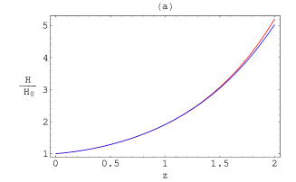
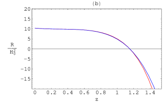
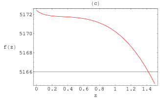
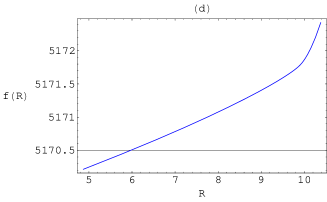
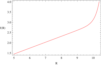
The complexity involved in the expression on the r.h.s of (35) does not permit an analytical solution for $f(z)$. However, since the expressions are true only for small $z$ we can always look for an approximation. Note that the expressions of $H(z)$, $R(z)$ and $\frac{df}{dz}$ given by (33), (34) and (35) contain an exponential term each. Retaining the terms up to the sixth power of $z$ in the series expansion of the exponentials and using them in (35) an analytical form of $f(z)$ can be obtained. The analytical expression, however, is not being mentioned here for economy of space. Instead variation of $f(z)$ versus $z$ under the above approximation is plotted in fig.1. That such an approximation holds good in our range of interest ($0\leq z\leq 1.15$) is also clear from fig.1(a)and (b) where we find that the curves for $H(z)$ and $R(z)$ drawn with and without the approximation appears almost indistinguishable at low redshifts. A parametric plot of $R$ and $f$ with $z$ as parameter, is then plotted in fig.1(d)to obtain the nature of variation of $f(R)$ against $R$.

Thus in order to address the coincidence problem in this model the function $f(R)$ should be such that, at low redshift it behaves like the curve given in fig.1(d). The plot shows that the function $f(R)$ which is initially linear in nature for $z\geq 0.5$ implying no interaction with matter sector, attains a non linear character in the very recent past $z\leq 0.5$ facilitating the interaction and hence a transition from deceleration to an accelerated phase of expansion of the Universe. It is always possible to suggest an analytic function that can match the behavior of $f(R)$ as plotted in fig.1(d) but we must remember that any such choice that fits the curve does not guarantee $\dot{r}=0$. For example the function

$$f(R)=\lambda_{1}R+\lambda_{2}R^{n}$$ (36)

when plotted against $R$ appears to behave similarly (shown in fig.2).

The behavior of $\dot{r}$ for the above choice of $f(R)$ however deviates from desirable features. For this reason we refrain from suggesting any $f(R)$ but stress on the fact that such a function can always be found in principle that not only fits the curve but also guarantees $\dot{r}=0$, thereby alleviating the coincidence problem.

Figure 1: The plots $(a)$ and $(b)$ show the variation of actual and approximate expressions of $H(z)$ and $R(z)$ vs. $z$ in red and blue respectively for model I with $q_{0}=-0.73$ and $q^{\prime}=1.5$. The curves appear to match exactly at low redshifts. Variation of $f(z)$ vs. $z$ and $f(R)$ vs. $R$ are shown in $(c)$ and $(d)$ respectively with $f^{\prime}_{0}=2$ and $H_{0}=1$ units.

Figure 2: The curve shows the plot of $f(R)$ vs.$R$ as given in equation (36) for $\lambda_{1}=0.29$, $\lambda_{2}=2.25\times 10^{-41}$ and $n=40$.

5 Model II

Another parametrization of $q(z)$ common in literature is of the form[24]

$$q(z)=\frac{1}{2}+\frac{q_{1}z+q_{2}}{(1+z)^{2}}$$ (37)

where $q_{1}$ and $q_{2}$ are constants with ($\frac{1}{2}+q_{2}$) giving the present value of the deceleration parameter and $\frac{dq}{dz}|_{z=0}=q_{1}-2q_{2}$. For a spatially flat Robertson-Walker Universe the best fit to the pair of parameters is ($q_{1}$, $q_{2}$) = (1.47, -1.46) and the transition redshift for these set of values is $z_{t}=0.36$[25]. For high redshifts $z\gg 1$, the deceleration parameter $q$ remains fixed at $\frac{1}{2}$ in this model.

Proceeding in exactly the same manner as in section (4) we get

$$H(z)=H_{0}(1+z)^{\frac{3}{2}}\exp\left[\frac{q_{2}}{2}+\frac{q_{1}z^{2}-q_{2}}{2(1+z)^{2}}\right]$$ (38)

$$R(z)=6H_{0}^{2}(1+z)^{3}\left(\frac{1}{2}-\frac{q_{1}z+q_{2}}{(1+z)^{2}}\right)\exp\left[q_{2}+\frac{q_{1}z^{2}-q_{2}}{(1+z)^{2}}\right]$$ (39)

$$\mbox{and}\hskip 28.45274pt\frac{df}{dz}=f^{\prime}_{0}\exp\left[\frac{-2(2q_{1}z+q_{1}+q_{2})}{(1+z)^{2}}\right]\frac{dR}{dz}$$ (40)

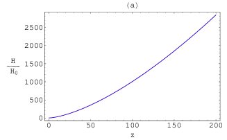
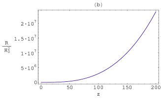
Obtaining an analytical solution for $f(z)$ from equation (40) is difficult in this case as well. However, following similar approximation in the exponential terms of the above equations, as in the previous model, a solution for $f(z)$ can be easily obtained and the nature of the function is shown in fig.3 along with the variations of $H(z)$ and $R(z)$ against $z$. The plots of $H(z)$ and $R(z)$ with and without the approximations are found to be almost indistinguishable over a long range of $z$ justifying the approximation. Nevertheless, the parametric plot in fig.4 shows that the function $f(R)$ in this case is double valued in the recent phase of evolution of the Universe.

Figure 3: The plots $(a)$ and $(b)$ show the variation of actual and approximate expressions of $H(z)$ and $R(z)$ vs. $z$ in red and blue respectively for model II with $q_{1}=1.47$ and $q_{2}=-1.46$. The curves appear to match exactly over a long range of redshift. Variation of $f(z)$ vs. $z$ is shown in $(c)$ for $f^{\prime}_{0}=2$ and $H_{0}=1$ units.

Figure 4: Plot of $f(R)$ vs. $R$ for model II with $q_{1}=1.47$, $q_{2}=-1.46$ and $f^{\prime}_{0}=2$ in $H_{0}=1$ units.

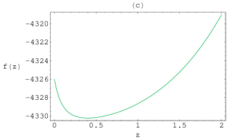
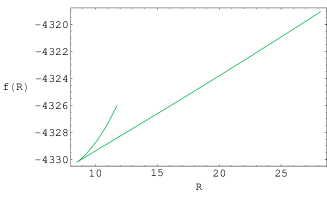
Therefore, for the particular parametrization of $q(z)$ chosen in (37), one cannot obtain a suitable well behaved function $f(R)$, capable of alleviating the coincidence problem. This result in contrast with that obtained in[21] can be understood if we notice that a prior choice of $f(R)$ fixes the functional behavior of $q$ and hence that of $q^{\prime}$. In[21] $f(R)$ is chosen by hand and the present value of $q$ is used to fix the parameters in the given $f(R)$, but it fails to achieve the correct value of $q^{\prime}|_{z=0}$ in the process. Our approach on the other hand, is just opposite. We fix the function $q$ that fits with observational data and look for a suitable $f(R)$ that can alleviate the coincidence problem. We find that no such $f(R)$ exists as long we restrict ourselves to $q$ that behaves as given in (37).

6 Conclusions

A suitable kind of interaction between dark energy and dark matter can make the ratio of their densities possible to attain a stationary value during the course of evolution and consequently can help alleviating the coincidence problem. In Einstein gravity such interactions are phenomenological and needs fine tuning of the interaction term. On the other hand, in Einstein frame representation of $f(R)$ gravity models, the interaction between the dark energy (scalar partner of the metric tensor) and dark matter is fixed by the conformal transformation. In this present article we address coincidence problem in the context of $f(R)$ gravity in Einstein frame. We point out that fixing the functional form of any one of the four quantities viz. the Hubble parameter, the matter density, the scalar field or the potential (or any derived quantity like the deceleration parameter ) shall in principle suffice to determine the functional form of all other quantities including $f(R)$. We choose two functional forms for deceleration parameter readily available in literature those fit observational data. The linear function $q(z)$ in Model I determines the the functional behavior of $f(R)$ for low redshift which is plotted in fig.1(d). The plot shows that the function $f(R)$ which is initially linear in nature for $z\geq 0.5$ implying no interaction with matter sector, attains a non linear character in the very recent past $z\leq 0.5$ facilitating the interaction and hence a transition from deceleration to an accelerated phase of expansion of the Universe. In another attempt a popular non-linear function of $q(z)$ is chosen for investigation. However the function $f(R)$ obtained in this case is double valued at low redshifts and hence is not suitable from physical point of view. Thus our investigation rules out the possibility of such form of deceleration parameter in $f(R)$ gravity if one is looking for a model free from coincidence problem.

References

-
[1]
Riess, A. G., et.al., Astron. J., 116, 1009(1998)
Perlmutter, S. et.al., Astrophys. J., 517, 565(1999). -
[2]
Spergel, D. N., et al.,Astrophys. J. Suppl., 148, 175 (2003)
Spergel, D. N., et al., Astrophys. J. Suppl., 170, 377 (2007)
Komatsu, E., et al., Astrophys. J. Suppl., 180, 330 (2009). -
[3]
Eisenstein, D. J., et al., Astrophys. J., 633, 560 (2005)
Percival, W. J., Cole, S. , Eisenstein, D. J., Nichol, R. C., Peacock, J. A., Pope, A. C. and Szalay, A. S., Mon. Not. Roy. Astron. Soc., 381, 1053 (2007)
Percival, W. J., et al., Mon. Not. Roy. Astron. Soc., 401, 2148 (2010). -
[4]
Carvalho, J. C., Lima, J. A. S. and Waga, I., Phys. Rev., D 46, 2404(1992).
Wetterich, C., Astron. Astrophys., 301, 321(1995).
Arbab, A. I., Gen. Rel. Grav., 29, 61(1997).
Padmanabhan, T., gr-qc/0112068.
Vishwakarma, R. G., Class. Quantum Grav., 19, 4747(2002).
Dutta Choudhury, S. B. and Sil, A., Astrophys. Space Sci., 301, 61(2006). -
[5]
Fujii, Y., Phys. Rev. D, 26, 2580 (1982).
Ford, L. H., Phys. Rev. D 35, 2339 (1987).
Wetterich, C., Nucl. Phys B., 302, 668 (1988).
Ratra, B. and Peebles, J. , Phys. Rev D, 37, 321 (1988).
Chiba, T., Sugiyama, N. and Nakamura, T., Mon. Not. Roy. Astron. Soc., 289, L5 (1997).
Ferreira, P. G. and Joyce, M., Phys. Rev. Lett., 79, 4740 (1997).
Ferreira, P. G. and Joyce, M., Phys. Rev. D, 58, 023503 (1998).
Copeland, E. J. , Liddle, A. R. and Wands, D., Phys. Rev. D, 57, 4686 (1998).
Caldwell, R. R., Dave, R. and Steinhardt, P. J., Phys. Rev. Lett., 80, 1582 (1998).
Zlatev, I., Wang, L. M. and Steinhardt, P. J., Phys. Rev. Lett., 82, 896 (1999).
Steinhardt, P. J., Wang, L. M. and Zlatev, I., Phys. Rev. D, 59, 123504 (1999). -
[6]
Chiba, T., Okabe, T. and Yamaguchi, M., Phys. Rev. D, 62, 023511 (2000).
Armendariz-Picon, C., Mukhanov, V. F. and Steinhardt, P. J., Phys. Rev. Lett., 85, 4438 (2000).
Armendariz-Picon, C., Mukhanov, V. F. and Steinhardt, P. J., Phys. Rev. D, 63, 103510 (2001). - [7] Turner, M.S., astro-ph/0108103 (2001).
[8]
Caldwell, R.R., Phys. Lett. B, 545, 23(2002)
Caldwell, R.R., Kamionkowski, M., and Weinberg, N.N., Phys. Rev. Lett., 91, 071301(2003). -
[9]
Vikman, A., Phys. Rev. D, 71, 023515 (2005)
Guo, Z., Piao, Y., Zhang, X., and Zhang, Y., Phys. Lett. B, 608, 177(2005)
Zhang, X.F., Li, H., Piao, Y.S., and Zhang, X.M., Mod. Phys. Lett. A, 21, 231(2006)
Perivolaropoulos, L., Phys.Rev. D, 71, 063503(2005)
Wei, H., and Cai, R.G., Class. Quant. Grav. , 22, 3189(2005)
Li, M.z., Feng, B., and Zhang, X.m, J. Cosmol. Astropart. Phys., 0512, 002 (2005)
Stefancic, H., Phys. Rev. D 71 124036(2005)
Anisimov, A., Babichev, E., and Vikman, A., J. Cosmol. Astropart. Phys. , 0506 006(2005)
Wang, B., Gong, Y.g., and Abdalla, E., Phys. Lett. B, 624 141(2005)
Nojiri, S., and Odintsov, S.D., Gen. Rel. Grav. , 38, 1285(2006)
Aref’eva, I.Y., Koshelev, A.S., and Vernov, S.Y., Phys. Rev. D, 72, 064017(2005)
Zhao, G.B., Xia, J.Q., Li, M., Feng, B., and Zhang, X., Phys. Rev. D, 72, 123515(2005)
Tsujikawa, S., Phys. Rev. D, 72, 083512(2005) -
[10]
Copeland, E. J., Sami M. and Tsujikawa, S., Int. J. Mod. Phys., D 15, 1753(2006)
Frieman, J., Turner, M., Huterer, D., Ann.Rev.Astron.Astrophys., 46, 385(2008), arxiv:0803.0982[astro-ph]
Tsujikawa, S., arXiv:1004.1493 [astro-ph]; Li, M. et.al, Commun.Theor.Phys., 56, 525(2011), arXiv:1103.5870 [astro-ph.CO] -
[11]
Buchdahl, H.A., Mon. Not. Roy. Astron. Soc., 150,
1(1970) Kerner, R., Gen. Rel. Grav. , 14, 453(1982)
Duruisseau, J.P., Kerner, R., and Eysseric, P., Gen. Rel. Grav. , 15, 797(1983)
Barrow, J.D., and Ottewill, A.C., J. Phys. A: Math. Gen. , 16, 2757(1983) - [12] Starobinsky, A.A., Phys. Lett. B, 91, 99(1980).
- [13] Carroll, S.M., Duvvuri, V., Trodden, M., and Turner, M.S., Phys. Rev. D, 70, 043528(2004).
- [14] Amendola, L., Polarski, D., and Tsujikawa, S., Phys. Rev. Lett., 98, 131302(2007).
[15]
Chiba, T., it Phys. Lett. B, 575, 1(2003)
Erickcek, A.L., Smith, T.L., and Kamionkowski, it M., Phys. Rev. D, 74, 121501(2006)
Chiba, T., Smith, T.L., and Erickcek, A.L., it Phys. Rev. D, 75, 124014(2007)
Nojiri, S., and Odintsov, S.D., it Phys. Lett. B, 659, 8212008
Capozziello, S., Stabile, A., and Troisi, A., it Phys. Rev. D, 76, 104019(2007)
Capozziello, S., Stabile, A., and Troisi, A., it Class. Quant. Grav. , 25, 085004(2008)
Olmo, G.J., it Phys. Rev. D, 75, 023511(2007). -
[16]
Hu, W., and Sawicki, I., Phys. Rev. D, 76, 064004(2007)
Nojiri, S., and Odintsov, S.D., Phys. Rev. D, 68, 123512(2003)
Faraoni, V., Phys. Rev. D, 74, 023529(2006)
Faulkner, T., Tegmark, M., Bunn, E.F., and Mao, Y., Phys. Rev. D, 76, 063505(2007)
Zhang, P.J., Phys. Rev. D, 76, 024007(2007)
Capozziello, S., and Tsujikawa, S., Phys. Rev. D, 77, 107501(2008)
Sawicki, I., and Hu, W., Phys. Rev. D, 75, 127502(2007)
Amendola, L., and Tsujikawa, S., Phys. Lett. B, 660, 125(2008). -
[17]
S. Nojiri and S. D. Odintsov, Phys.Rept., 59, 505(2011)
T. P. Sotiriou and V. Faraoni, Rev. Mod. Phys., 82, 451(2010)
S. Capozziello and V. Faraoni, ”Beyond Einstein Gravity”, Springer, 2010
F. S. N. Lobo, arXiv:0807.1640 [gr-qc] - [18] N. Arkani-Hamed, L. J. Hall, C. Kolda, H. Murayama, Phys. Rev. Lett 85, 4434(2000)
[19]
del campo, S., Herrera, R., Pavon, D., Phys.Rev.D, 78,
021302(2008)
Nojiri, S., Odintsov, S.D., Phys.Lett.B, 637, 139(2006)
Hu, B., Ling, Y., Phys.Rev.D, 73, 123510(2006)
Wai, H., Rong-Gen Cai, Phys.Rev.D71, 043504(2005)
Avelino, P.P., Phys.Lett. B, 611, 15(2005)
Scherrer, R.J. Phys.Rev. D, 71, 063519(2005)
Chimento, L.P., Jacubi, A.S., Pavon, D., Zimdahl, W., Phys.Rev. D, 67, 083513(2003)
Pietroni, M., Phys.Rev.D, 67, 103523(2003) -
[20]
W. Zimdahl, D. Pavon and L. P. Chimento, Phys. Lett., B 521, 133(2001)
W. Zimdahl and D. Pavn, Gen. Rel. Grav., 35, 413(2003)
S. D. Campo, R. Herrera and D. Pavon, JCAP, 0901, 020(2009)
C. Wetterich, Astron. Astrophys., 301, 321(1995)
L. Amendola, Phys. Rev. D, 62, 043511(2000)
D. Tocchini-Valentini and L. Amendola, Phys. Rev. D ,65, 063508(2002)
C. G. Boehmer, G. Caldera-Cabral, R. Lazkoz and R. Maartens, Phys. Rev. D, 78, 023505(2008) - [21] Y. Bisabr, Phys. Rev. D, 82, 124041(2010)
- [22] Riess, A. G., et.al., Astrophys. J., 607, 665(2004).
- [23] Cunha, J. V., Phys. Rev. D, 79, 047301(2009).
- [24] Gong, Y. G. and Wang, A. Phys. Rev. D, 73, 083506 (2006).
- [25] Gong, Y. G. and Wang, A. Phys. Rev. D, 75, 043520 (2007).