∎
22email: rao.tushar@nsitonline.in 33institutetext: S. Srivastava 44institutetext: Indraprastha Institute of Technology, Delhi, India
44email: saket@iiitd.ac.in
Twitter Sentiment Analysis: How To Hedge Your Bets In The Stock Markets
Abstract
Emerging interest of trading companies and hedge funds in mining social web has created new avenues for intelligent systems that make use of public opinion in driving investment decisions. It is well accepted that at high frequency trading, investors are tracking memes rising up in microblogging forums to count for the public behavior as an important feature while making short term investment decisions. We investigate the complex relationship between tweet board literature (like bullishness, volume, agreement etc) with the financial market instruments (like volatility, trading volume and stock prices). We have analyzed Twitter sentiments for more than 4 million tweets between June 2010 and July 2011 for DJIA, NASDAQ-100 and 11 other big cap technological stocks. Our results show high correlation (upto 0.88 for returns) between stock prices and twitter sentiments. Further, using Granger’s Causality Analysis, we have validated that the movement of stock prices and indices are greatly affected in the short term by Twitter discussions. Finally, we have implemented Expert Model Mining System (EMMS) to demonstrate that our forecasted returns give a high value of R-square (0.952) with low Maximum Absolute Percentage Error (MaxAPE) of 1.76% for Dow Jones Industrial Average (DJIA). We introduce a novel way to make use of market monitoring elements derived from public mood to retain a portfolio within limited risk state (highly improved hedging bets) during typical market conditions.
Keywords:
Stock market sentiment analysis Twitter microblogging social network analysis1 INTRODUCTION
Financial analysis and computational finance have been an active area of research for many decadesLee1999357 . Over the years, several new tools and methodologies have been developed that aim to predict the direction as well as range of financial market instruments as accurately as possibleGuresen201110389 . Before the emergence of internet, information regarding company’s stock price, direction and general sentiments took a long time to disseminate among people. Also, the companies and markets took a long time (weeks or months) to calm market rumors, news or false information (memes in Twitter context). Web is characterized with fast pace information dissemination as well as retrieval danah_article . Spreading good or bad information regarding a particular company, product, person etc. can be done at the click of a mouse Brown:2002:SLI:560498 , Acemoglu2010194 or even using micro-blogging services such as TwitterBBC_twitter . Recently scholars have made use of twitter feeds in predicting box office revenues Asur_Huberman_2010 , political game wagons Tumasjan_Sprenger_Sandner_Welpe_2010 , rate of flu spread Szomszor_Kostkova_Quincey_2009 and disaster news spread tweet_disaster . For short term trading decisions, short term sentiments play a very important role in short term performance of financial market instruments such as indexes, stocks and bonds morning_paper .
Early works on stock market prediction can be summarized to answer the question - Can stock prices be really predicted? There are two theories - (1) random walk theory (2) and efficient market hypothesis (EMH)Hong . According to EMH stock index largely reflect the already existing news in the investor community rather than present and past prices. On the other hand, random walk theory argues that the prediction can never be accurate since the time instance of news is unpredictable. A research conducted by Qian et.al. compared and summarized several theories that challenge the basics of EMH as well as the random walk model completelyQian . Based on these theories, it has been proven that some level of prediction is possible based on various economic and commercial indicators. The widely accepted semi-strong version of the EMH claims that prices aggregate all publicly available information and instantly reflect new public versionBurton_m . It is well accepted that news drive macro-economic movement in the markets, while researches suggests that social media buzz is highly influential at micro-economic level, specially in the big indices like DJIA Bollen_Mao_Zeng_2010 , Bollen_second_paper , Gilbert_Karahalios_2010 and Sprenger . Through earlier researches it has been validated that market is completely driven by sentiments and bullishness of the investor’s decisions Qian . Thus a comprehensive model that could incorporate these sentiments as a parameter is bound to give superior prediction at micro-economic level.
Earlier work done by Bollen et. al. shows how collective mood on Twitter (aggregate of all positive and negative tweets) is reflected in the DJIA index movements Bollen_Mao_Zeng_2010 and Bollen_second_paper . In this work we have applied simplistic message board approach by defining bullishness and agreement terminologies derived from positive and negative vector ends of public sentiment w.r.t. each market security or index terms (such as returns, trading volume and volatility). Proposed method is not only scalable but also gives more accurate measure of large scale investor sentiment that can be potentially used for short term hedging strategies as discussed ahead in section 6. This gives clear distinctive way for modeling sentiments for service based companies such as Google in contrast to product based companies such as Ebay, Amazon and Netflix. We validate that Twitter feed for any company reflects the public mood dynamics comprising of breaking news and discussions, which is causative in nature. Therefore it adversely affects any investment related decisions which are not limited to stock discussions or profile of mood states of entire Twitter feed.
In section 2, we discuss the motivation of this work and related work in the area of stock market prediction in section 3. In section 4 we explain what and how of the techniques used in mining data and explain the terminologies used in market and tweet board literature. In section 5 we have given prediction methods used in this model with the forecasting results. In section 6 we discuss how Twitter based model can be used for improving hedging decisions in a diversified portfolio by any trader. Finally in section 7 we discuss the results and in section 8 we present the future prospects and conclude the work.
2 MOTIVATION
”Communities of active investors and day traders who are sharing opinions and in some case sophisticated research about stocks, bonds and other financial instruments will actually have the power to move share prices …making Twitter-based input as important as any other data to the stock”
-TIME (2009) TIME09
High Frequency Trading (HFT) comprises of very high percentage of trading volumes in the present US market. Traders make an investment position that is held only for very brief periods of time - even just seconds - and rapidly trades into and out of those positions, sometimes thousands or tens of thousands of times a day. Therefore the value of an investment is as good as last known index price. Investors will do anything that will give them an advantage in placing market bets. A large percentage of high frequency traders in US markets, have trained AI bots to capture buzzing trends in the social media feeds without learning dynamics of the sentiment and accurate context of the deeper information being diffused in the social networks. For example, in February 2011 during Oscars when Anne Hathaway was trending, stock prices of Berkshire Hathaway rose by 2.94% Hathaway Figure 1 highlight the incidents when the stock price of Berkshire Hathaway jumped coinciding with an increase of buzz on social networks/ micro-blogging websites regarding Anne Hathaway (for example during movie releases).

The events are marked as red points in the Figure 1 , event specific news on the points-
A: Oct. 3, 2008 - Rachel Getting Married opens: BRK.A up 0.44%
B: Jan. 5, 2009 - Bride Wars opens: BRK.A up 2.61%
C: Feb. 8, 2010 - Valentine’s Day opens: BRK.A up 1.01%
D: March 5, 2010 - Alice in Wonderland opens: BRK.A up 0.74%
E: Nov. 24, 2010 - Love and Other Drugs opens: BRK.A up 1.62%
F: Nov. 29, 2010 - Anne announced as co-host of the Oscars: BRK.A up 0.25%
G: Feb. 28. 2011 - Anne hosts Oscars with James Franco: BRK.A up 2.94%
As seen in this example, large volume of tweets can create short term influential effects on stock prices. Events such as these motivate us to investigate deeper relationship between the dynamics of social media messages and market movements Lee1999357 . This work is not directed to find a new stock prediction technique which will counter in the effects of various other macroeconomic factors.
The aim of this work, is to quantitatively evaluate the effects of twitter sentiment dynamics around a stocks indices/stock prices and use it in conjunction with the standard model to improve the accuracy of prediction. Further in section 6 we investigate into how tweets can be very useful in identifying trends in futures and options markets and to build hedging strategies to protect one’s investment position in the shorter term.
3 RELATED WORK
There have been several works related to web mining of data (blogposts, discussion boards and news) Ant_frank , Bagnoli199927 , Gilbert_Karahalios_2010 and to validate the significance of assessing behavioral changes in the public mood to track movements in stock markets. Some trivial work shows information from investor communities is causative of speculation regarding private and forthcoming information and commentarieslerman , Wysocki_1998 ,Das_chen and Da_Engelberg_Gao_2010 . Dewally in 2003 worked upon naive momentum strategy confirming recommended stocks through user ratings had significant prior performance in returns Dewally . But now with the pragmatic shift in the online habits of communities around the worlds, platforms like StockTwits111http://stocktwits.com/ Business_week and TweetTrader222http://tweettrader.net/ have come up and their usage is virally spreading out. Das and Chen made the initial attempts by using natural language processing algorithms classifying stock messages based on human trained samples. However their result did not carried statistically significant predictive relationships Das_chen .
Gilbert et.al. and Zhang et.al. have used corpus from livejournal blogposts in assessing the bloggers sentiment in dimensions of fear , anxiety and worry making use of Monte Carlo simulation to reflect market movements in S&P 500 index Gilbert_Karahalios_2010 ; Zhang_Fuehres_Gloor_2009 . Similar and significantly accurate work is done by Bollen et. al who used dimensions of Google- Profile of Mood States to reflect changes in closing price of DJIA Bollen_Mao_Zeng_2010 . Sprengers et.al. analyzed individual stocks for S&P 100 companies and tried correlating tweet features about discussions of the stock discussions about the particular companies containing the Ticker symbol Sprenger . However these approaches have been restricted to community sentiment at macro-economic level which doesn’t give explanatory dynamic system for individual stock index for companies. Thus deriving a model that is scalable for individual stocks/ companies and can be exploited to make successful hedging strategies as discussed in section 6.
4 WEB MINING AND DATA PROCESSING
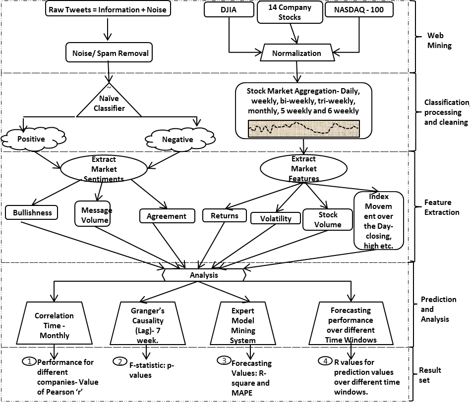
In this section we describe our method of Twitter and financial data collection as shown in Figure 2. In the first phase, we mine the tweet data and after removal of spam/noisy tweets, they are subsequently subjected to sentiment assessment tools in phase two. In later phases feature extraction, aggregation and analysis is done.
4.1 Tweets Collection and Processing
Out of other investor forums and discussion boards, Twitter has widest acceptance in the financial community and all the messages are accessible through a simple search of requisite terms through an application programming interface (API)333Twitter API is easily accessible through an easy documentation available at- https://dev.twitter.com/docs. Also Gnip - http://gnip.com/twitter, the premium platform available for purchasing public firehose of tweets has many investors as financial customers researching in the area.. Sub forums of Twitter like StockTwits and TweetTrader have emerged recently as hottest place for investor discussion buy/sell out at voluminous rate. Efficient mining of sentiment aggregated around these tweet feeds provides us an opportunity to trace out relationships happening around these market sentiment terminologies. Currently more than 250 million messages are posted on Twitter everyday (Techcrunch October 2011444http://techcrunch.com/2011/10/17/twitter-is-at-250-million-tweets-per-day/).
This study was conducted over a period of 14 months period between June 2nd 2010 to 29th July 2011. During this period, we collected 4,025,595 (by around 1.08M users) English language tweets Each tweet record contains (a) tweet identifier, (b) date/time of submission(in GMT), (c) language and (d)text. Subsequently the stop words and punctuation are removed and the tweets are grouped for each day (which is the highest time precision window in this study since we do not group tweets further based on hours/minutes). We have directed our focus DJIA, NASDAQ-100 and 11 major companies listed in Table 1. These companies are some of the highly traded and discussed technology stocks having very high tweet volumes.
| Company Name | Ticker Symbol |
|---|---|
| Amazon | AMZN |
| Apple | AAPL |
| AT&T | T |
| Dell | DELL |
| EBay | EBAY |
| GOOG | |
| Microsoft | MSFT |
| Oracle | ORCL |
| Samsung Electronics | SSNLF |
| SAP | SAP |
| Yahoo | YHOO |
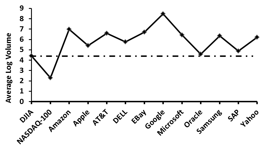
As seen in Figure 3, the average message volume for the 11 companies used to validate the working model; is more than the average discussion volume of DJIA and NASDAQ-100. In this study we have observed that technology stocks generally have a higher tweet volume than non-technology stocks. One reason for this may be that all technology companies come out with new products and announcements much more frequently than companies in other sectors(say infrastructure, energy, FMCG, etc.) thereby generating greater buzz on social media networks. However, our model may be applied to any company/indices that generate high tweet volume.
4.2 Sentiment Classification
In order to compute sentiment for any tweet we had to classify each incoming tweet everyday into positive or negative using na ve classifier. For each day total number of positive tweets is aggregated as while total number of negative tweets as . We have made use of JSON API from Twittersentiment 555https://sites.google.com/site/twittersentimenthelp/, a service provided by Stanford NLP research group Alec_Bhayani . Online classifier has made use of Naive Bayesian classification method, which is one of the successful and highly researched algorithms for classification giving superior performance to other methods in context of tweets. Their classification training was done over a dataset of 1,600,000 tweets and achieved an accuracy of about 82.7%. These methods have high replicability and few arbitrary fine tuning elements.
In our dataset roughly 61.68% of the tweets are positive, while 38.32% of the tweets are negative for the company stocks under study. The ratio of 3:2 indicates stock discussions to be much more balanced in terms of bullishness than internet board messages where the ratio of positive to negative ranges from 7:1 Dewally to 5:1 Ant_frank . Balanced distribution of stock discussion provides us with more confidence to study information content of the positive and negative dimensions of discussion about the stock prices on microblogs.
4.3 Tweet Feature Extraction
One of the research questions this study explores is how investment decisions for technological stocks are affected by entropy of information spread about companies under study in the virtual space. Tweet messages are micro-economic factors that affect stock prices which is quite different type of relationship than factors like news aggregates from traditional media, chatboard room etc. which are covered in earlier studies over a particular period Dewally , lerman and Ant_frank . Keeping this in mind we have only aggregated the tweet parameters (extracted from tweet features) over a day. In order to calculate parameters weekly, bi-weekly, tri-weekly, monthly, 5 weekly and 6 weekly we have simply taken average of daily twitter feeds over the requisite period of time.
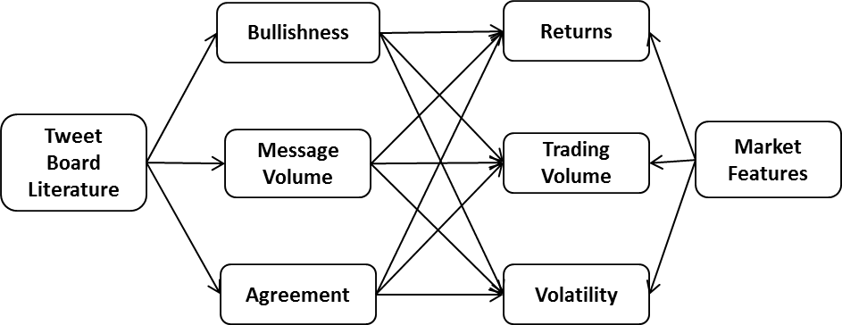
Twitter literature in perspective of stock investment is summarized in Figure 4. We have carried forward work of Antweiler et.al. for defining bullishness () for each day (or time window) given equation as:
| (1) |
Where and represent number of positive or negative tweets on a particular day . Logarithm of bullishness measures the share of surplus positive signals and also gives more weight to larger number of messages in a specific sentiment (positive or negative). Message volume for a time interval t is simply defined as natural logarithm of total number of tweets for a specific stock/index which is . The agreement among positive and negative tweet messages is given by:
| (2) |
If tweet messages about a particular company are bullish or bearish,
agreement would be in that case. Influence of silent tweets days
in our study (trading days when no tweeting happens about
particular company) is less than which is significantly less
than previous research Ant_frank ; Sprenger . Carried terminologies
for all the tweet features{Positive, Negative, Bullishness, Message Volume, Agreement}
remain same for each day with the lag of one day. For example, carried bullishness
for day is given by .
4.4 Financial Data Collection
We have downloaded financial stock prices at daily intervals from Yahoo Finance API666http://finance.yahoo.com/ for DJIA, NASDAQ-100 and the companies under study given in Table 1. The financial features (parameters) under study are opening () and closing () value of the stock/index, highest () and lowest () value of the stock/index and returns. Returns are calculated as the difference of logarithm to the base between the closing values of the stock price of a particular day and the previous day.
| (3) |
Trading volume is the logarithm of number of traded shares. We estimate daily volatility based on intra-day highs and lows using Garman and Klass volatility measures Garman_Klass given by the formula:
| (4) |
5 STATISTICAL ANALYSIS AND RESULTS
We begin our study by identifying the correlation between the Twitter feed features and stock/index parameters which give the encouraging values of statistically significant relationships with respect to individual stocks(indices). To validate the causative effect of tweet feeds on stock movements we have used econometric technique of Granger’s Casuality Analysis. Furthermore, we make use of expert model mining system (EMMS) to propose an efficient prediction model for closing price of DJIA and NASDAQ . Since this model does not allow us to draw conclusion about the accuracy of prediction (which will differ across size of the time window) subsequently discussed later in this section.
5.1 Correlation Matrix
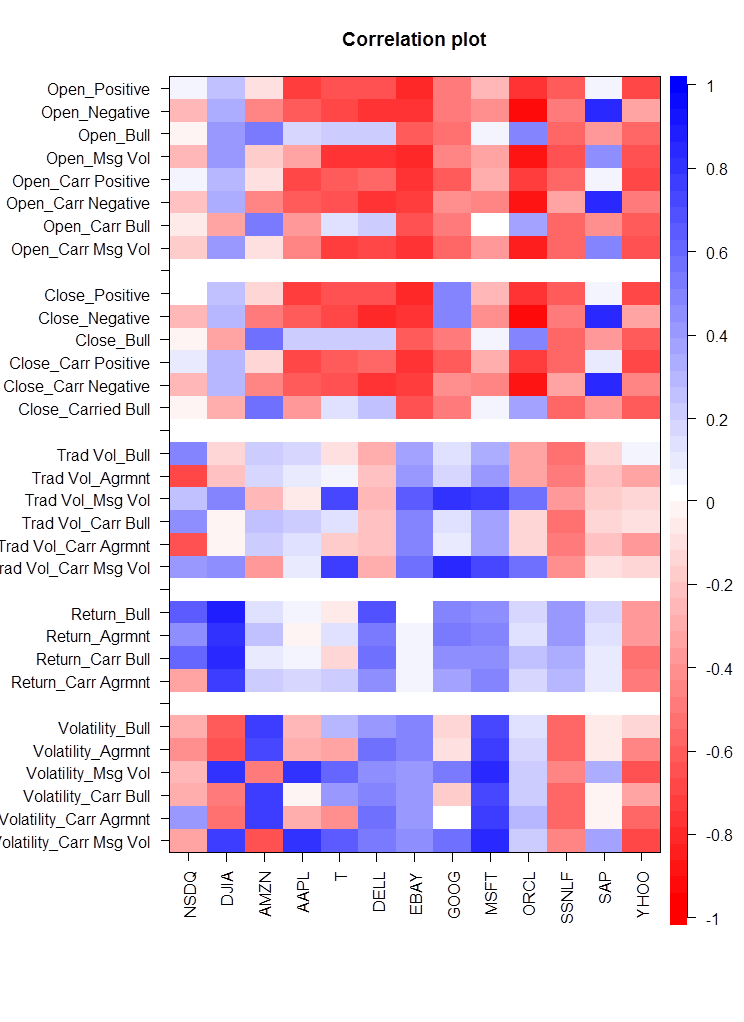
For the stock indices DJIA and NASDAQ and 11 tech companies under study we have come up with the correlation matrix given in Figure 10 in the appendix between the financial market and Twitter sentiment features explained in section 4. Financial features for each stock/index (Open, Close, Return, Trade Volume and Volatility) is correlated with Twitter features (Positive, Negative, Bullishness, Carried Positive, Carried Negative and Carried Bullishness).The time period under study is monthly average as it the most accurate time window that gives significant values as compared to other time windows which is discussed later section 5.4.
Our approach shows strong correlation values between various features (upto for opening price of Oracle and for returns from DJIA index etc.) and the average value of correlation between various features is around . Comparatively highest correlation values from earlier work has been around Sprenger . As the relationships between the stock(index) parameters and Twitter features show different behavior in magnitude and sign for different stocks(indices), a uniform standardized model would not applicable to all the stocks(indices). Therefore, building an individual model for each stock(index) is the correct approach for finding appreciable insight into the prediction techniques. Trading volume is mostly governed by agreement values of tweet feeds as for same day agreement and for DJIA. Returns are mostly correlated to same day bullishness by and by lesser magnitude for the carried bullishness for DJIA. Volatility is again dependent on most of the Twitter features, as high as for same day message volume for NASDAQ-100.
One of the anomalies that we have observed is that EBay gives negative correlation between the all the features due to heavy product based marketing on Twitter which turns out as not a correct indicator of average growth returns of the company itself.
| Index | Lag | Positive | Negative | Bull | Agrmnt | Msg Vol | Carr Positive | Carr Negative | Carr Bull | Carr Agrmnt | Carr Msg Vol |
|---|---|---|---|---|---|---|---|---|---|---|---|
| DJIA | 1 | 0.614 | 0.122 | 0.891 | 0.316 | 0.765 | 0.69 | 0.103 | 0.785 | 0.759 | 0.934 |
| 2 | 0.033** | 0.307 | 0.037** | 0.094* | 0.086** | 0.032** | 0.301** | 0.047** | 0.265 | 0.045** | |
| 3 | 0.219 | 0.909 | 0.718 | 0.508 | 0.237 | 0.016** | 0.845 | 0.635 | 0.357 | 0.219 | |
| 4 | 0.353 | 0.551 | 0.657 | 0.743 | 0.743 | 0.116 | 0.221 | 0.357 | 0.999 | 0.272 | |
| 5 | 0.732 | 0.066 | 0.651 | 0.553 | 0.562 | 0.334 | 0.045** | 0.394 | 0.987 | 0.607 | |
| 6 | 0.825 | 0.705 | 0.928 | 0.554 | 0.732 | 0.961 | 0.432 | 0.764 | 0.261 | 0.832 | |
| 7 | 0.759 | 0.581 | 0.809 | 0.687 | 0.807 | 0.867 | 0.631 | 0.987 | 0.865 | 0.969 | |
| NSDQ | 1 | 0.106 | 0.12 | 0.044** | 0.827 | 0.064* | 0.02** | 0.04** | 0.043** | 0.704 | 0.071* |
| 2 | 0.048** | 0.219 | 0.893 | 0.642 | 0.022** | 0.001** | 0.108 | 0.828 | 0.255 | 0.001** | |
| 3 | 0.06* | 0.685 | 0.367 | 0.357 | 0.135 | 0.01** | 0.123 | 0.401 | 0.008** | 0.131 | |
| 4 | 0.104 | 0.545 | 0.572 | 0.764 | 0.092* | 0.194 | 0.778 | 0.649 | 0.464 | 0.343 | |
| 5 | 0.413 | 0.997 | 0.645 | 0.861 | 0.18 | 0.157 | 0.762 | 0.485 | 0.945 | 0.028 | |
| 6 | 0.587 | 0.321 | 0.421 | 0.954 | 0.613 | 0.795 | 0.512 | 0.898 | 0.834 | 0.591 | |
| 7 | 0.119 | 0.645 | 0.089 | 0.551 | 0.096 | 0.382 | 0.788 | 0.196 | 0.648 | 0.544 |
5.2 Bivariate Granger Causality Analysis
The results in previous section show strong correlation between financial market parameters and Twitter sentiments. However, the results also raise a point of discussion: Whether market movements affects Twitter sentiments or Twitter features causes changes in the markets? To verify this hypothesis we make use of Granger Causality Analysis (GCA) to the time series averaged to weekly time window to returns through DJIA and NASDAQ-100 with the Twitter features (positive, negative, bullishness, message volume and agreement). GCA is not used to establish causality, but as an economist tool to investigate a statistical pattern of lagged correlation. A similar observation that cloud precede rain is widely accepted; proving cloud may may contain something that causes rain but itself may not be actual causative of the real event.
GCA rests on the assumption that if a variable X causes Y then changes in X will be systematically occur before the changes in Y. We realize lagged values of X shall bear significant correlation with Y. However correlation is not necessarily behind causation. We have made use of GCA in similar fashion as Bollen_Mao_Zeng_2010 ; Gilbert_Karahalios_2010 This is to test if one time series is significant in predicting another time series. Let returns be reflective of fast movements in the stock market. To verify the change in returns with the change in Twitter features we compare the variance given by following linear models in equation 5 and equation 6 -
| (5) |
| (6) |
Equation 5 uses only ’’ lagged values of , i.e. ( ) for prediction, while Equation 6 uses the lagged values of both and the tweet features time series given by , . . . , . We have taken weekly time window to validate the casuality performance, hence the lag values 777lag at k for any parameter M at week is the value of the parameter prior to week. For example, value of returns for the month of April, at the lag of one month will be which will be will be calculated over the weekly intervals .
From the Table 2, we can reject the null hypothesis that the Twitter features do not affect returns in the financial markets i.e. with a high level of confidence (high p-values). However as we see the result applies to only specific negative and positive tweets (** for p-value and * for p-value which is 95% and 99% confidence interval respectively). Other features like agreement and message volume do not have significant casual relationship with the returns of a stock index (low p-values).
5.3 EMMS Model for Forecasting
We have used Expert Model Mining System (EMMS) which incorporates a set of competing methods such as Exponential Smoothing (ES), Auto Regressive Integrated Moving Average (ARIMA) and seasonal ARIMA models. These methods are widely used in financial modeling to predict the values of stocks/bonds/commodities/etc Pegels ; Box . These methods are suitable for constant level, additive trend or multiplicative trend and with either no seasonality, additive seasonality, or multiplicative seasonality.
In this work, selection criterion for the EMMS is coefficient of determination (R squared) which is square of the value of pearson-’r’ of fit values (from the EMMS model) and actual observed values. Mean absolute percentage error (MAPE) and maximum absolute percentage error (MaxAPE) are mean and maximum values of error (difference between fit value and observed value in percentage). To show the performance of tweet features in prediction model, we have applied the EMMS twice - first with tweets features as independent predictor events and second time without them. This provides us with a quantitative comparison of improvement in the prediction using tweet features.
ARIMA (p,d,q) are in theory and practice, the most general class of models for forecasting a time series data, which is subsequently stationarized by series of transformation such as differencing or logging of the series . For a non-seasonal ARIMA (p,d,q) model- p is autoregressive term, d is number of non-seasonal differences and q is the number of lagged forecast errors in the predictive equation. A stationary time series differences times has stochastic component
| (7) |
Where and are the mean and variance of normal distribution, respectively. The systematic component is modeled as:
| (8) |
Where, the lag-p observations from the stationary time series with associated parameter vector and the lagged errors of order q, with associated parameter vector. The expected value is the mean of simulations from the stochastic component,
| (9) |
| Index | Predictors | Model Fit statistics | Ljung-Box Q(18) | ||||
|---|---|---|---|---|---|---|---|
| R-squared | MaxAPE | Direction | Statistics | DF | Sig. | ||
| Dow-30 | Yes | 0.95 | 1.76 | 90.8 | 11.36 | 18 | 0.88 |
| No | 0.92 | 2.37 | 60 | 9.9 | 18 | 0.94 | |
| NASDAQ-100 | Yes | 0.68 | 2.69 | 82.8 | 23.33 | 18 | 0.18 |
| No | 0.65 | 2.94 | 55.8 | 16.93 | 17 | 0.46 | |
Seasonal ARIMA model is of form ARIMA (p ,d ,q) (P,D,Q) where P specifies the seasonal autoregressive order, D is the seasonal differencing order and Q is the moving average order. Another advantage of EMMS model is that it automatically selects the most significant predictors among all others that are available.
In the dataset we have time series for a total of approximately 60 weeks (422 days), out of which we use approximately 75% i.e. 45 weeks for the training both the models with and without the predictors for the time period June 2nd 2010 to April 14th 2011. Further we verify the model performance as one step ahead forecast over the testing period of 15 weeks from April 15th to 29th July 2011 which count for wide and robust range of market conditions. Forecasting accuracy in the testing period is compared for both the models in each case in terms of maximum absulute percentage error (MaxAPE), mean absolute percentage error (MAPE) and the direction accuracy. MAPE is given by the equation 10, where is the predicted value and is the actual value.
| (10) |
While direction accuracy is measure of how accurately market or commodity up/ down movement is predicted by the model, which is technically defined as logical values for respectively.
As we can see in the Table 3, there is significant reduction in MaxAPE for DJIA(2.37 to 1.76) and NASDAQ-100 (2.96 to 2.69) when EMMS model is used with predictors as events which in our case our all the Tweet features (positive, negative, bullishness, message volume and agreement). Using tweet features as part of the prediction process in the EMMS model, gives more robust approach than the traditional forecasting methods. There is significant decrease in the value of MAPE for DJIA which is in our case than for earlier approaches Bollen_Mao_Zeng_2010 . As we can from the values of R-square, MAPE and MaxAPE in Table 3 for both DJIA and NASDAQ , our proposed model uses Twitter sentiment analysis for a superior performance over traditional methods. Since EMMS is a customizable and scalable technique, our proposed model is bound to perform well in a wide range of stocks and indices.
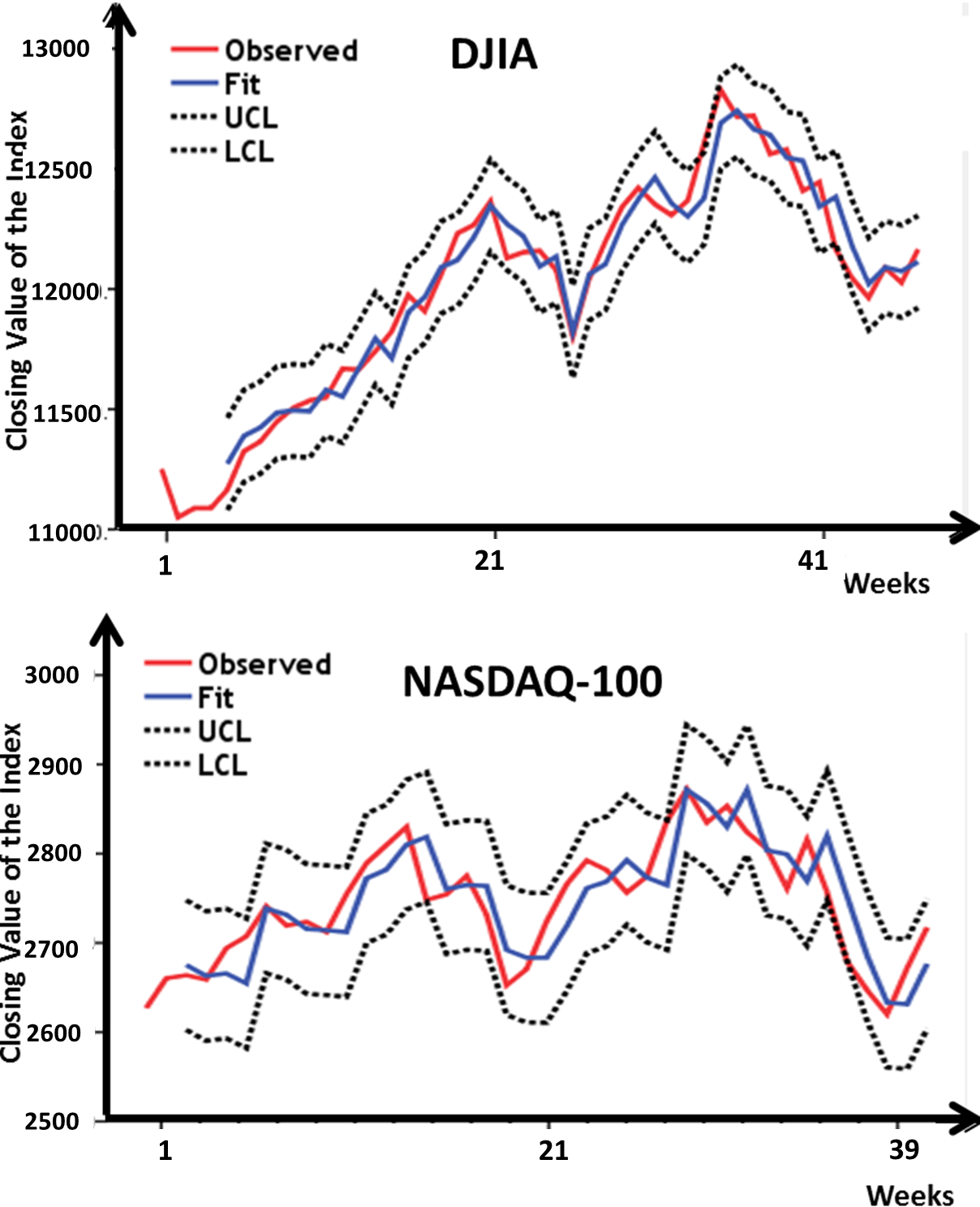
Figures 5 shows the EMMS model fit for weekly closing values for DJIA and NASDAQ . In the figure fit are model fit values, observed are values of actual index and UCL & LCL are upper and lower confidence limits of the prediction model.
5.4 Prediction Accuracy using OLS Regression
Our results in the previous section showed that forecasting performance of stocks/indices using Twitter sentiments varies for different time windows. Hence it is important to quantitatively deduce a suitable time window that will give us most accurate prediction. Figure 6 shows the plot of R-square metric for OLS regression for returns from stock indexes NASDAQ-100 and DJIA from tweet board features (like number of positive, negative, bullishness, agreement and message volume) both for carried (at 1-day lag) and same week.
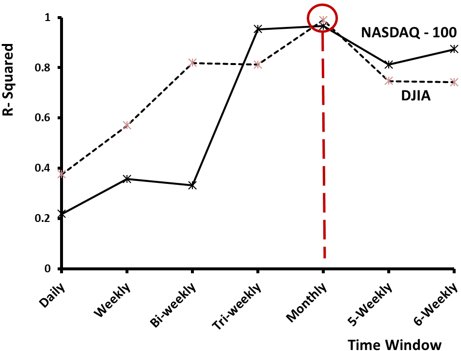
The R-square metric (explained in section 5.3) is calculated as prediction performance indicator for different time windows from daily, weekly, bi-weekly to 6 weekly time window. From the figure 6 it can be inferred as we increase the time window the accuracy in prediction increases but only till a certain point that is monthly in our case beyond which value of R-square starts decreasing again. Thus, for monthly predictions we have highest accuracy in predicting anomalies in the returns from the tweet board features.
In the next section we will discuss the practical implementation of how short term hedging strategies can improve efficiency by modeling mass public opinion and behavior for a particular company or stock index through mining of tweet sentiments.
6 HEDGING STRATEGY USING TWITTER SENTIMENT ANALYSIS
Portfolio protection is very important practice that is weighted as much as portfolio appreciation. Just like a normal user purchases insurance for its house, car or any commodity, one can also buy insurance for the investment that is made in the stock securities. This doesn’t prevent a negative event from happening, but if it does happen and you’re properly hedged, the impact of the event is reduced. In a diverse portfolio hedging against investment risk means strategically using instruments in the market to offset the risk of any adverse price movements. Technically, to hedge investor invests in two securities with negative correlations, which again in itself is time varying dynamic statistics.
To explain how weekly forecast based on mass tweet sentiment features can be potentially useful for a singular investor, we will take help of a simple example.
Let us assume that the share for a company C1 is available for $X per share and the cost of premium for a stock option of company C1 (with strike price $X) is $Y.
A total amount invested in shares of a company C1 which is number of shares (let it be N) $X
B= total amount invested in put option of company C1 (relevant blocksize $Y)
And always for an effective investment (N $X) ( Blocksize $Y)
An investor shall choose the value of N as per as their risk appetitive i.e. ratio of A:B 2:1 (assumed in our example, will vary from from investor to investor). Which means in the rising market conditions, he would like to keep 50% of his investment to be completely guarded, while rest 50% are risky components; whereas in the bearish market condition he would like to keep his complete investment fully hedged by buying put options equivalent of all the investment he has made in shares for the same security. From Figure 7, we infer for the P/L curves consisting of shares and 2 different put options for the company C1 purchased as different time intervals 888The reason behind purchase of long put options at different time intervals is because in a fully hedged portfolio, profit arrow has lower slope as compared to partially hedged portfolio (refer P/L graph). Thus the trade off between risk and security has to be carefully played keeping in mind the precise market conditions.; hence the different premium price even with the same strike price of $X. Using married put strategy makes the investment risk free but reduces the rate of return in contrast to the case which comprises of only equity security which is completely free-fall to the market risk. Hence the success of married put strategy depends greatly on the accuracy of predicting whether the markets will rise of fall. Our proposed Tweet sentiment analysis can be highly effective in this prediction to determine accurate instances when the investor should readjust his portfolio before the actual changes happen in the market. Our proposed approach provides an innovative technique of using dynamic Twitter sentiment analysis toexploit the collective wisdom of the crowd for minimising the risk in a hedged portfolio. Below we summarize two different portfolio states at different market conditions.
| Partially Hedged Portfolio at 50% risk |
|---|
| 1000 shares at price of $X 1000X |
| 1 Block size of 500 shares put options purchased at strike price of $X with premium of $Y each 500Y |
| Total= 1000X + 500Y |
| Fully Hedged Portfolio at minimized risk |
| 1000 shares at price of $X 1000X |
| 2 Block size of 500 shares each put options purchased at strike price of $X with premium of $Y each 2500Y 1000Y |
| Total 1000X 1000Y |

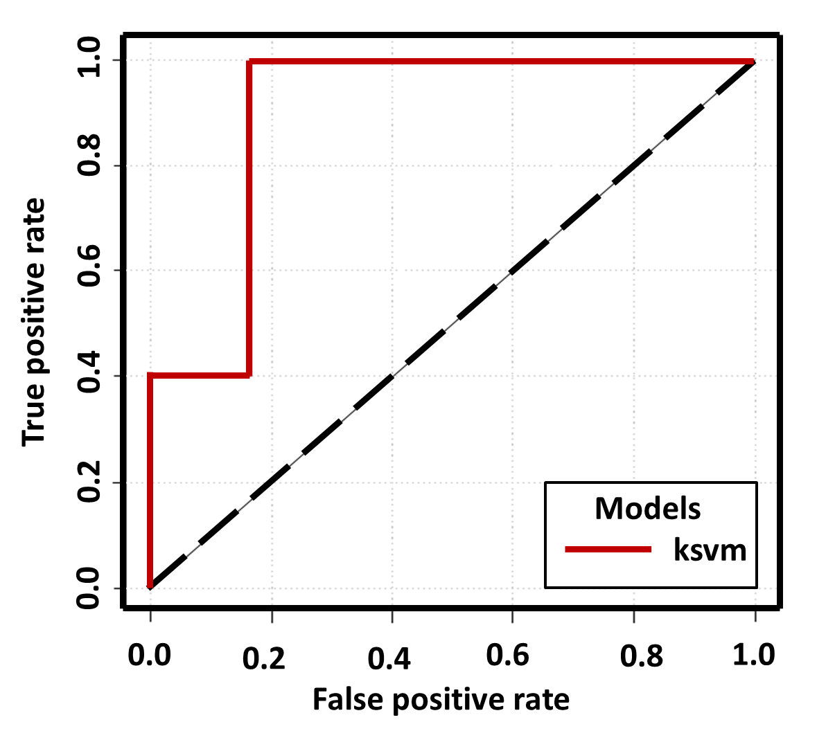
To check the effectiveness of our proposed tweet based hedging strategy, we run simulations and make portfolio adjustments in various market conditions (bullish, bearish, volatile etc). To elaborate, we take an example of DJIA ETF’s as the underlying security over the time period of 14th November 2010 to 30th June 2011. Approximately 76% of the time period is taken in the training phase to tune the SVM classifier (using tweet sentiment features from the prior week). This trained SVM classifier is then used to predict market direction (DJIA’s index movement) in the coming week. Testing phase for the classification model (class 1- bullish market and class 0- bearish market ) is from 8th May to 30th June 2011 consisting a total of 11 weeks. SVM model is build using KSVM classification technique with the linear (vanilladot) kernel using the package ’e1071’ in R statistical language. Over the training dataset, the tuned value of the objective function is obtained as and the number of support vectors is . Confusion matrix for the predicted over the actual values (in percentage) is given in Table 5. Overall classifier accuracy over the testing phase is . Receiver operator characteristics (ROC) curve measuring the accuracy of the classifier as true positive rate to false positive rate is given in the figure 8. It shows the tradeoff between sensitivity i.e. true positive rate and specificity i.e. true negative rate (any increase in sensitivity will be accompanied by a decrease in specificity). Good statistical significance for the classification accuracy can be inferred from the value of area under the ROC curve (AUC) which comes out to .
| Confusion Matrix | Predicted Direction | ||
|---|---|---|---|
| Market Down | Market Up | ||
| Actual Direction | Market Down | 45 | 9 |
| Market Up | 0 | 45 | |
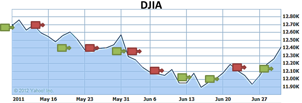
Figure 9 shows the DJIA index during the testing period and the arrows mark the weeks when the adjustment is done in the portfolio based on prediction obtained from tweet sentiment analysis of prior week. At the end of the week (on Sunday), using tweet sentiment feature we predict what shall be the market condition in the coming week- whether the prices will go down or up. Based on the prediction portfolio adjustment - bearish bullish or bullish bearish.
7 DISCUSSIONS
In section 5, we observed how the statistical behavior of market through Twitter sentiment analysis provides dynamic window to the investor behavior. Furthermore, in the section 6 we discussed how behavioral finance can be exploited in portfolio decisions to make highly reduced risked investment. Our work answers the important question - If someone is talking bad/good about a company (say Apple etc.) as singular sentiment irrespective of the overall market movement, is it going to adversely affect the stock price? Among the 5 observed Twitter message features both at same day and lagged intervals we realize only some are Granger causative of the returns from DJIA and NASDAQ-100 indexes, while changes in the public sentiment is well reflected in the return series occurring at even lags of and weeks. Remarkably the most significant result is obtained for returns at lag 2 (which can be inferred as possible direction for the stock/index movements in the next week).
Table 6 given below explains the different approaches to the problem that have been done in past by researchers Sprenger , Bollen_Mao_Zeng_2010 and Gilbert_Karahalios_2010 . As can be seen from the table, our approach is scalable, customizable and verified over a large data set and time period as compared to other approaches. Our results are significantly better than the previous work. Furthermore, this model can be of effective use in formulating short-term hedging strategies (using our proposed Twitter based prediction model).
| Previous Approaches | Bollen et al. Bollen_Mao_Zeng_2010 and Gilbert et al. Gilbert_Karahalios_2010 | Sprenger et al. Sprenger | This Work |
|---|---|---|---|
| Approach | Mood of complete Twitter feed | Stock Discussion with ticker $ on Twitter | Discussion based tracking of Twitter sentiments |
| Dataset | 28th Feb 2008 to 19th Dec 2008, 9M tweets sampled as 1.5% of Twitter feed | 1st Jan 2010 to 30th June 2010- 0.24M tweets | 2nd June 2010 to 29th July 2011- 4M tweets through search API |
| Techniques | SOFNN, Grangers and linear models | OLS Regression and Correlation | Corr, GCA, Expert Model Mining System (EMMS) |
| Results | * 86.7% directional accuracy for DJIA | * Max corr value of 0.41 for returns of S&P 100 stocks | * High corr values (upto -0.96) for opening price Strong corr values (upto 0.88) for returns MaxAPE of 1.76% for DJIA Directional accuracy of 90.8% for DJIA |
| Feedback/ Drawbacks | Individual modeling for stocks not feasible | News not taken into account, very less tweet volumes | Comprehensive and customizable approach. Can be used for hedging in F&O markets |
8 CONCLUSION
In this paper, we have worked upon identifying relationships between Twitter based sentiment analysis of a particular company/index and its short-term market performance using large scale collection of tweet data. Our results show that negative and positive dimensions of public mood carry improved power to track movements of individual stocks/indices. We have also investigated various other features like how previous week sentiment features control the next week’s opening, closing value of stock indexes for various tech companies and major index like DJIA and NASDAQ-100. As compared to earlier approaches in the area which have been limited to wholesome public mood and stock ticker constricted discussions, we verify strong performance of our alternate model that captures mass public sentiment towards a particular index or company in scalable fashion and hence empower a singular investor to ideate coherent relative comparisons. Our analysis of individual company stocks gave strong correlation values (upto 0.88 for returns) with twitter sentiment features of that company. Further we also discuss how Twitter sentiments bring wisdom of the crowd to use by even a singular investor in the form of simplistic married put hedging strategy. Using this technique trader can retain his portfolio with minimum risk even during highly bullish/bearish market conditions. It is no surprise that this approach is far more robust and gives far better results (upto 91% directional accuracy) than any previous work. In the near future, Twitter sentiments analysis promises to be an effective strategy for hedging the investments in the financial markets.
References
- [1] Daron Acemoglu, Asuman Ozdaglar, and Ali ParandehGheibi. Spread of (mis)information in social networks. Games and Economic Behavior, 70(2):194 – 227, 2010.
- [2] Sitaram Asur and Bernardo A Huberman. Predicting the future with social media. Computing, 25(1):492 499, 2010.
- [3] The Atlantic. Does anne hathaway news drive berkshire hathaway’s stock?, 2011. This is an electronic document. Date of publication: [March 18 2011]. Date retrieved: October 12, 2011. Date last modified: [Date unavailable].
- [4] Mark Bagnoli, Messod D. Beneish, and Susan G. Watts. Whisper forecasts of quarterly earnings per share. Journal of Accounting and Economics, 28(1):27 – 50, 1999.
- [5] Johan Bollen, Huina Mao, and Xiao-Jun Zeng. Twitter mood predicts the stock market. Computer, 1010(3003v1):1–8, 2010.
- [6] George Edward Pelham Box and Gwilym Jenkins. Time Series Analysis, Forecasting and Control. Holden-Day, Incorporated, 1990.
- [7] danah m. boyd and Nicole B. Ellison. Social network sites: Definition, history, and scholarship. Journal of Computer-Mediated Communication, 13(1):210–230, 2007.
- [8] John Seely Brown and Paul Duguid. The Social Life of Information. Harvard Business School Press, Boston, MA, USA, 2002.
- [9] Zhi Da, Joseph Engelberg, and Pengjie Gao. In search of attention. Russell The Journal Of The Bertrand Russell Archives, (919), 2010.
- [10] Sanjiv R. Das and Mike Y. Chen. Yahoo! for Amazon: Sentiment Parsing from Small Talk on the Web. SSRN eLibrary, 2001.
- [11] Micha l Dewally. Internet investment advice: Investing with a rock of salt. Financial Analysts Journal, 59(4):65–77, 2003.
- [12] S. Doan, B.-K. H. Vo, and N. Collier. An analysis of Twitter messages in the 2011 Tohoku Earthquake. ArXiv e-prints, September 2011.
- [13] Murray Z. Frank and Werner Antweiler. Is All That Talk Just Noise? The Information Content of Internet Stock Message Boards. SSRN eLibrary, 2001.
- [14] Mark B. Garman and Michael J. Klass. On the estimation of security price volatilities from historical data. The Journal of Business, 53(1):67–78, 1980.
- [15] Eric Gilbert and Karrie Karahalios. Widespread worry and the stock market. Artificial Intelligence, pages 58–65, 2010.
- [16] Alec Go, Richa Bhayani, and Lei Huang. Twitter Sentiment Classification using Distant Supervision.
- [17] Erkam Guresen, Gulgun Kayakutlu, and Tugrul U. Daim. Using artificial neural network models in stock market index prediction. Expert Systems with Applications, 38(8):10389 – 10397, 2011.
- [18] K.H. Lee and G.S. Jo. Expert system for predicting stock market timing using a candlestick chart. Expert Systems with Applications, 16(4):357 – 364, 1999.
- [19] Alina Lerman. Individual Investors’ Attention to Accounting Information: Message Board Discussions. SSRN eLibrary, 2011.
- [20] Huaxia Rui Liangfei Qiu and Andrew Whinston. A twitter-based prediction market: Social network approach. ICIS 2011 Proceedings. Paper 5, 2011.
- [21] Burton G. Malkiel. The efficient market hypothesis and its critics. Journal of Economic Perspectives, 17(1):59–82, 2003.
- [22] Huina Mao, Scott Counts, and Johan Bollen. Predicting financial markets: Comparing survey,news, twitter and search engine data. Quantitative Finance Papers 1112.1051, arXiv.org, December 2011.
- [23] Garth P. McCormick. Communications to the editor exponential forecasting: Some new variations. Management Science, 15(5):311–320, 1969.
- [24] Douglas McIntyre. Turning wall street on its head, 2009. This is an electronic document. Date of publication: [May 29, 09]. Date retrieved: September 24, 2011. Date last modified: [Date unavailable].
- [25] Hong Miao, Sanjay Ramchander, and J. K. Zumwalt. Information Driven Price Jumps and Trading Strategy: Evidence from Stock Index Futures. SSRN eLibrary, 2011.
- [26] BBC News. Twitter predicts future of stocks, 2011. This is an electronic document. Date of publication: [April 6, 2011]. Date retrieved: October 21, 2011. Date last modified: [Date unavailable].
- [27] Bo Qian and Khaled Rasheed. Stock market prediction with multiple classifiers. Applied Intelligence, 26:25–33, February 2007.
- [28] Timm O. Sprenger and Isabell M. Welpe. Tweets and Trades: The Information Content of Stock Microblogs. SSRN eLibrary, 2010.
- [29] Martin Szomszor, Patty Kostkova, and Ed De Quincey. swineflu : Twitter predicts swine flu outbreak in 2009. 3rd International ICST Conference on Electronic Healthcare for the 21st Century eHealth2010, (December), 2009.
- [30] Andranik Tumasjan, Timm O Sprenger, Philipp G Sandner, and Isabell M Welpe. Predicting elections with twitter: What 140 characters reveal about political sentiment. International AAAI Conference on Weblogs and Social Media Washington DC, pages 178–185, 2010.
- [31] Peter Wysocki. Cheap talk on the web: The determinants of postings on stock message boards. Working Paper, 1998.
- [32] Max Zeledon. Stocktwits may change how you trade, 2009. This is an electronic document. Date of publication: [2009]. Date retrieved: September 01, 2011. Date last modified: [Date unavailable].
- [33] Xue Zhang, Hauke Fuehres, and Peter A Gloor. Predicting stock market indicators through twitter i hope it is not as bad as i fear. Anxiety, pages 1–8, 2009.
9 APPENDIX
Correlation heatmap indicative of significant relationships between various twitter features with the index features.
