Kernel Estimation from Salient Structure for Robust Motion Deblurring

Abstract

Blind image deblurring algorithms have been improving steadily in the past years. Most state-of-the-art algorithms, however, still cannot perform perfectly in challenging cases, especially in large blur setting. In this paper, we focus on how to estimate a good blur kernel from a single blurred image based on the image structure. We found that image details caused by blur could adversely affect the kernel estimation, especially when the blur kernel is large. One effective way to remove these details is to apply image denoising model based on the Total Variation (TV). First, we developed a novel method for computing image structures based on TV model, such that the structures undermining the kernel estimation will be removed. Second, we applied a gradient selection method to mitigate the possible adverse effect of salient edges and improve the robustness of kernel estimation. Third, we proposed a novel kernel estimation method, which is capable of removing noise and preserving the continuity in the kernel. Finally, we developed an adaptive weighted spatial prior to preserve sharp edges in latent image restoration. Extensive experiments testify to the effectiveness of our method on various kinds of challenging examples.

1 Introduction

Blind image deblurring is a challenging problem which has drawn a lot of attention in recent years due to its involvement of many challenges in problem formulation, regularization, and optimization. The formation process of motion blur is usually modeled as

$$B=k\ast I+\varepsilon,$$ (1)

where $B$, $I$, $k$ and $\varepsilon$ represent the blurred image, latent image, blur kernel (a.k.a. point spread function, PSF) and the additive noise, respectively. $\ast$ denotes the convolution operator. It is a well-known ill-posed inverse problem, which requires regularization to alleviate its ill-posedness and stabilize the solution.

Recently, significant processes have been made in [1, 2, 3, 4, 5, 6, 7]. The success of these methods comes from two important aspects: the sharp edge restoration and noise suppression in smooth regions, which enable accurate kernel estimation.

However, blurred image with some complex structures or large blur will fail most of state-of-the-art blind deblurring methods. Taking Fig. 1(a) as an example, the motion blur is very large due to the camera shake. In addition, the blurred image also contains complex structures. As shown in Figs. 1(b) - (f), some state-of-the-art methods [1, 2, 3, 6, 7] have difficulty in restoring or selecting useful sharp edges for kernel estimation due to the large blur and complex structures. Thus, the correct blur kernels are not obtained. This inevitably makes the final deblurred results unreliable.

Figure 1: A challenging example. (a) Blurred image. (b) Result of Shan et al. [2]. (c) Result of Cho and Lee [1]. (d) Result of Xu and Jia [3]. (e) Result of Levin et al. [7]. (f) Result of Krishnan et al. [6]. (g) Our result. (h) Our final salient edges $\nabla S$ (detailed further below) visualized by using Poisson reconstruction method. The size of motion blur kernel is $45\times 45$.

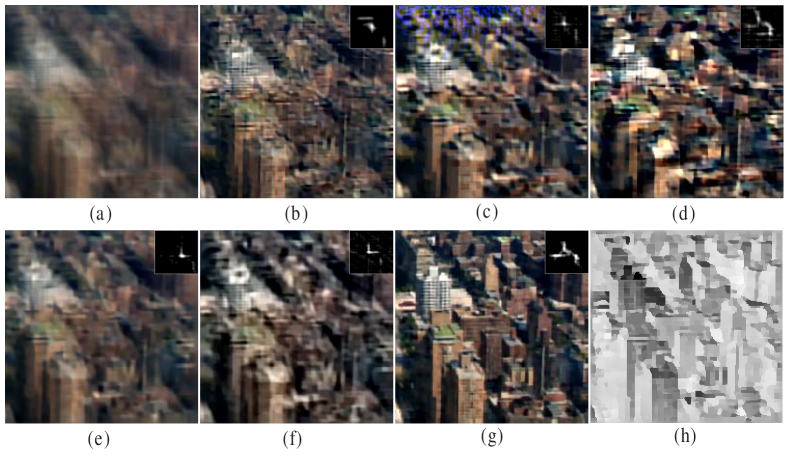
We address this issue and propose a new kernel estimation method based on the reliable structures. Our method is a new selection scheme to select reliable structures according to the image characteristics. Thus, it is able to get useful sharp edges for kernel estimation. Our deblurred result shown in Fig. 1(g) contains fine textures, and the kernel estimate is also better than others.

In addition, noisy kernels also damage the kernel estimation, which further leads to unreliable deblurred results. Therefore, removing noise in the kernels is also very important in kernel estimation.

Based on above analysis, we develop several strategies which are significantly different from previous works in the following aspects.

1. First, to remove detrimental structures and obtain useful information for kernel estimation, we develop a novel adaptive structure selection method which can choose reliable structures effectively.

2. To preserve the sparsity and continuity of blur kernels, we propose a new robust kernel estimation method by introducing a powerful spatial prior, which also helps remove the noise effectively.

3. Finally, we introduce a simple adaptive regularization term that combines the final salient structures to guide the latent image restoration, which is able to preserve sharp edges in the restored image.

We apply our method to some challenging examples, such as images with complex tiny structures or with large blur kernels, and verify that it is able to provide reliable kernel estimates which are noiseless and also satisfy the sparsity and continuity well. Moreover, high-quality final restored images can be obtained.

2 Related Work

Image deblurring is a hot topic in image processing and computer vision communities. In single image blind deblurring, early approaches usually imposed constraints on motion blur kernel and used parameterized forms for the kernels [8, 9]. Recently, Fergus et al. [4] adopted a zero-mean Mixture of Gaussian to fit for natural image gradients. A variational Bayesian method was employed to deblur an image. Shan et al. [2] used a certain parametric model to approximate the heavy-tailed natural image prior. Cai et al. [10] assumed that the latent images and kernels can be sparsely represented by an over-complete dictionary and introduced a framelet and curvelet system to obtain the sparse representation for images and kernels. Levin et al. [11] illustrated the limitation of the simple maximum a posteriori (MAP) approach, and proposed an efficient marginal likelihood approximation in [7]. Krishnan et al. [6] introduced a new normalized sparsity prior to estimate blur kernels. Goldstein and Fattal [12] estimated blur kernels by spectral irregularities. However, the kernel estimates of the aforementioned works usually contain some noise. The hard thresholding to the kernel elements method will destroy the inherent structure of kernels.

Another group methods [1, 3, 5, 13, 14] employed an explicit edge prediction step for kernel estimation. In [5], Joshi et al. computed sharp edges by first locating step edges and then propagating the local intensity extrema towards the edge. Cho et al. [14] detected sharp edges from blurred images directly and then the Radon transform was employed to estimate the blur kernel. However, these methods have difficulty in dealing with large blur. Cho and Lee [1] used bilateral filtering together with shock filtering to predict sharp edges iteratively and then selected the salient edges for kernel estimation. However, the Gaussian priors used in this method can not keep the sparsity of the motion blur kernel and the image structure. The final result usually contains noise. Xu and Jia [3] proposed an effective mask computation algorithm to adaptively select useful edges for kernel estimation. The kernel refinement was achieved by using iterative support detection (ISD) method [15]. However, this method ignores the continuity of the motion blur kernel. The estimated kernels contain some noise occasionally. Hu and Yang [16] learned good regions for kernel estimation and employed method [1] to estimate kernels. Although the performance is greatly improved, the sparsity and continuity of blur kernels still can not be guaranteed.

After obtaining the blur kernel, the blind deblurring problem becomes a non-blind deconvolution. Early approaches such as Wiener filter and Richardson-Lucy deconvolution [17] usually suffer from noise and ringing artifacts. Yuan et al. [18] proposed a progressive inter-scale and intra-scale based on the bilateral Richardson-Lucy method to reduce ringing artifacts. Recent works mainly focus on the natural image statistics [2, 19] to keep the properties of latent images and suppress ringing artifacts. Joshi et al. [20] used local color statistics derived from the image as a constraint to guide the latent images restoration. The works in [3, 21] used TV regularization to restore latent images, but the isotropic TV regularization will result in stair-casing effect.

It is noted that there also have been active researches on spatially-varying blind deblurring methods. Interested readers are referred to [22, 23, 24, 25, 26] for more details.

3 Kernel Estimation from Salient Structure

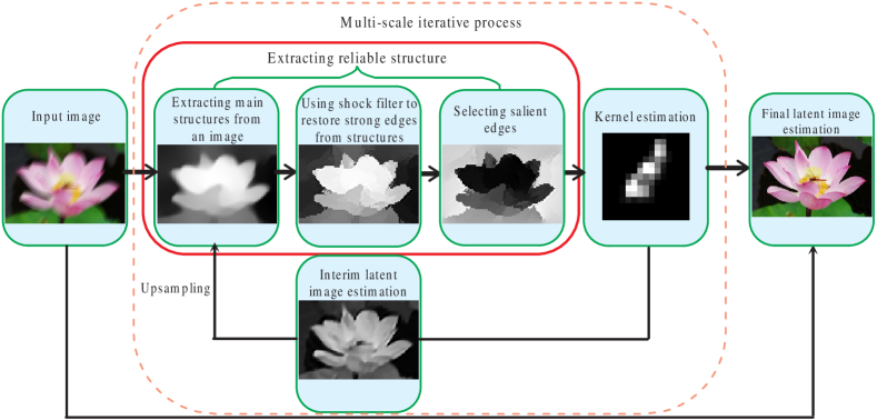
We find that different extraction of structure leads to different deblurred results, and extracting reliable structure is critical to deblurring. Thus, we focus on extracting more reliable structures, which is achieved by several key steps. First, we extract the main image structure (the first part of the solid red box in Fig. 2). Then, a shock filter is applied to get the enhanced structure (the second part of the solid red box in Fig. 2). Finally, some salient edges with large pixel values will be selected for the kernel estimation (the third part of the solid red box in Fig. 2). The details of this process will be discussed in Section 3.1, and the corresponding reasoning will be provided in Section 3.1.1.

It is noted that noisy interim kernels will also damage the interim latent image estimation, which further leads to unreliable kernels during the kernel refinement. We propose a robust kernel estimation method which combines the gradient properties of kernels to overcome this problem. Detailed analysis will be discussed in Section 3.2. The dotted line box shown in Fig. 2 encloses the process of kernel estimation in details.

Figure 2: The flowchart of our algorithm. The dotted line box encloses the process of kernel estimation.

3.1 Extracting Reliable Structure

Our method for adaptively selecting salient edges mainly relies on the idea of structure-texture decomposition method [27]. For an image $I$ with pixel intensity value $I(\textbf{x})$, the structure part is given by the optimizer of the following energy:

$$\min_{I_{s}}\sum_{\textbf{x}}\|\nabla I_{s}(\textbf{x})\|_{2}+\frac{1}{2\theta}(I_{s}(\textbf{x})-I(\textbf{x}))^{2},$$ (2)

where $\theta$ is an adjustable parameter. The image $I$ is decomposed into the structure component $I_{s}$ (shown in Fig. 3(c)) and the texture component $I_{T}=I-I_{s}$ (shown in Fig. 3(b)). The structure component $I_{s}$ contains the major objects in the image while $I_{T}$ includes fine-scale details and noise.

Figure 3: Different structures leading to different deblurred results. (a) Blurred image. (b) Texture component $I_{T}$. (c) Structure component $I_{s}$. (d) Results without performing model (2). (e) Results by using $I_{T}$ in the process of kernel estimation. (f) Results by using $I_{s}$ in the process of kernel estimation.

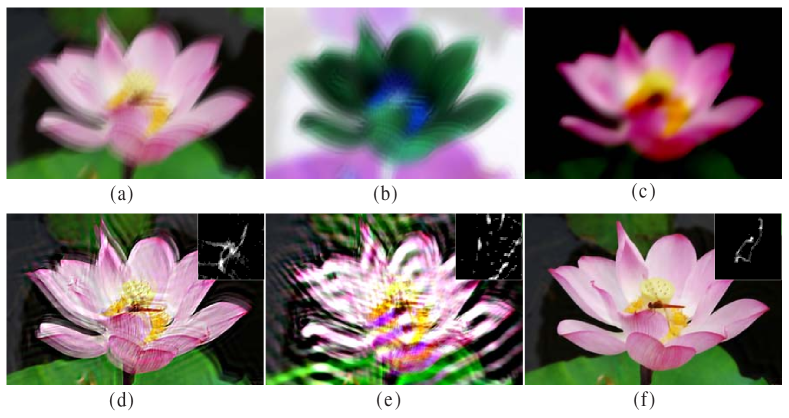
Fig. 3(f) demonstrates that the accuracy of kernel estimate is greatly improved by performing model (2). However, model (2) may lead to stair-casing effect in smooth area. This will cause gradient distortion and introduce inaccuracy for kernel estimation. A simple way to mitigate this effect is to adjust the value of $\theta$ to be large in the smooth areas, and small near the edges. To that end, we adopt the following adaptive model to select the main structure of an image $I$:

$$\min_{I_{s}}\sum_{\textbf{x}}\|\nabla I_{s}(\textbf{x})\|_{2}+\frac{1}{2\theta\omega(\textbf{x})}(I_{s}(\textbf{x})-I(\textbf{x}))^{2},$$ (3)

where $\omega(\textbf{x})=\exp(-|r(\textbf{x})|^{0.8})$ and $r(\textbf{x})$ is defined as

$$r(\textbf{x})=\frac{\|\sum_{\textbf{y}\in N_{h}(\textbf{x})}\nabla B(\textbf{y})\|_{2}}{\sum_{\textbf{y}\in N_{h}(\textbf{x})}\|\nabla B(\textbf{y})\|_{2}+0.5},$$ (4)

in which $B$ is the blurred image, and $N_{h}(\textbf{x})$ is an $h\times h$ window centered at pixel x. A small $r$ implies that the local region is flat, whereas large $r$ implies existing strong image structures in the local window. This equation is first employed by [3] to remove some narrow strips that may undermine the kernel estimation. However, model (3) keeps the similar advantages to those of [3] due to the adaptive weight $\omega(\textbf{x})$. It also has a strong penalty to these areas which are flat or contain narrow strips as well.

Figure 4: Comparison of results with models (2) and (3). (a) Blurred image and truth kernel. (b) Results with model (2). (c) Results with model (3). (d) Results of [3]. (e) - (h) Interim $\nabla S$ maps with model (2). (i) - (l) Interim $\nabla S$ maps with model (3). The final results (including the kernel estimate and deblurred result) shown in (c) performs better than others.

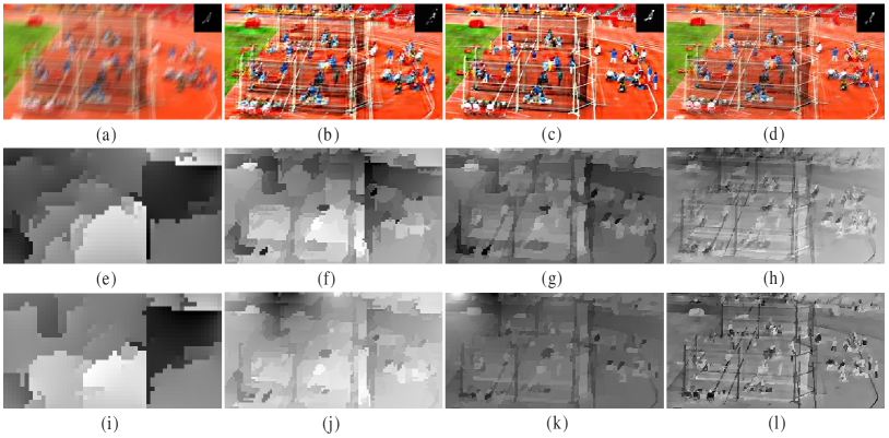
To demonstrate the validity of model (3), we conduct an experiment shown in Fig. 4. As shown in Fig. 4(a), the blurred image contains some complex structures, which may have detrimental effects on kernel estimation. Due to adopting the adaptive weight $\omega(\textbf{x})$ in model (3), kernel estimation result by model (3) is significantly better than that by model (2). Furthermore, compared with $\nabla S$ (detailed further below) maps shown in Figs. 4 (e) - (h) and Figs. 4 (i) - (l), both models (2) and (3) are able to select main structures of an image, but model (3) can retain some useful structures for kernel estimation.

After computing $I_{s}$, we compute the enhanced structure $\tilde{I_{s}}$ by a shock filter [28]:

$$\partial\tilde{I_{s}}/\partial t=-\text{sign}(\triangle\tilde{I_{s}})\|\nabla\tilde{I_{s}}\|_{2},$$ (5)

$$\tilde{I_{s}}|_{t=0}=I_{s},$$

where $\triangle I=I_{x}^{2}I_{xx}+2I_{x}I_{y}I_{xy}+I_{y}^{2}I_{yy}$.

Finally, we compute salient edges $\nabla S$ which will be used to guide the kernel estimation:

$$\nabla S=\nabla\tilde{I_{s}}H(\textbf{G},t),$$ (6)

where $H(\textbf{G},t)$ is the unit binary mask function which is defined as

$$H(\textbf{G},t)=\left\{\begin{array}[]{ll}1,&\mbox{}\ G_{i}\geqslant t,\\ 0,&\mbox{}\ $otherwise$,\end{array}\right.$$ (9)

and $\textbf{G}=(\|\nabla\tilde{I_{s}}\|_{2},\|\partial_{x}\tilde{I_{s}}\|_{1}/5\sqrt{2},\|\partial_{y}\tilde{I_{s}}\|_{1}/5\sqrt{2})$. The parameter $t$ is a threshold of the gradient magnitude $\|\nabla\tilde{I_{s}}\|_{2}$. By applying Eq. (6), some noise in the $\nabla\tilde{I_{s}}$ will be eliminated. Thus, only the salient edges with large values have influences on the kernel estimation.

It is noted that kernel estimation will be unreliable when a few salient edges are available for estimation. To solve this problem, we adopt several strategies as follows.

First, we adaptively set the initial values of $t$ according to the method of [1] at the beginning of the iterative deblurring process. Specifically, the directions of image gradients are initially quantized into four groups. $t$ is set to guarantee that at least $\frac{1}{2}\sqrt{N_{I}N_{k}}$ pixels participate in kernel estimation in each group, where $N_{I}$ and $N_{k}$ denote the total number of pixels in the input image and the kernel, respectively.

Then, as the iteration goes in the deblurring process, we gradually decrease the values of $\theta$ and $t$ at each iteration to include more edges for kernel estimation according to [3]. This adaptive strategy can allow for inferring subtle structures during kernel refinement.

Figs. 4 (e) - (l) show some interim $\nabla S$ maps in the iterative deblurring process. One can see that as the iteration goes, more and more sharp edges are included for kernel estimation.

3.1.1 Analysis on Structure Selection Method

To better understand our structure selection method, we use a 1D signal to provide more insightful analysis on how our method can help kernel estimation.

Figure 5: 1D signal illustration. The 1D signal (a) is decomposed into two main components: (b) structure component and (c) texture component by using model (3). (d) Sharp signal. Signals shown in this figure are obtained from an image scanline.

Given a signal (e.g., Fig. 5(a)), we can decompose it into the structure component (Fig. 5(b)) and texture component (Fig. 5(c)) by using model (3). For the structure component (Fig. 5(b)), we can use a shock filter and Eq. (6) to get a sharp signal (Fig. 5(d)) that is similar to the step signal. Step signal, however, usually succeeds in the kernel estimation, which has been proved by many previous works [11, 5]. In contrast, the texture component (Fig. 5(c)) usually fails in the kernel estimation. There are two mainly reasons: (1) The texture component contains noise which damages the kernel estimation; (2) The size of texture component is relatively small. Blurring reduces its peak height - that is, the shape of texture component is destroyed seriously after blur. Therefore, recovering the sharp version of texture component from the blurred version is a very difficult problem. As a result, a correct kernel estimate is hard to be obtained by texture component (e.g., Fig. 3(e)).

More generally, natural images can be regarded as 2D signals, which can be composed of many local 1D signals (Fig. 5(a)). This further demonstrates our method is valid. We have also performed lots of experiments to verify the validity of our method. The effectiveness of salient edges will be detailed in Section 3.5.

3.2 Kernel Estimation

The motion blur kernel describes the path of camera shake during the exposure. Most literatures assume that distributions of blur kernels can be well modeled by a Hyper-Laplacian, based on which the corresponding model for kernel estimation is

$$\min_{k}\|\nabla B-k*\nabla S\|_{2}^{2}+\gamma\|k\|_{\alpha}^{\alpha},$$

$$\text{s.t.}\quad k(\textbf{x})\geq 0,\quad\sum_{\textbf{x}}k(\textbf{x})=1,$$ (10)

where $0<\alpha\leqslant 1$.

Figure 6: Comparison of results with different spatial priors of motion blur kernel. In (a), the kernel estimate is obtained by using the kernel estimation model that is employed by [14]. The kernel estimate shown in (b) is obtained by using model (3.2). The kernel estimate shown in (c) is obtained by using model (3.2). (d), (e), and (f) show the iterations of kernel estimates by model in [14], model (3.2), and model (3.2), respectively. Deblurred result in (c) outperforms the result in (b) (e.g., the parts in the red boxes). The results (c) and (f) of our method are the best.

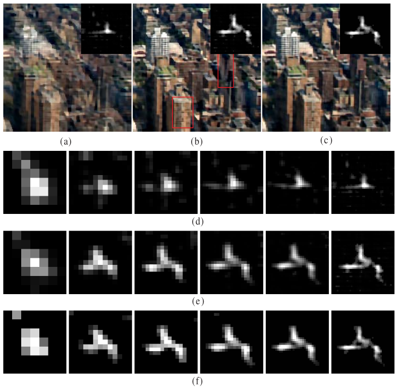
Although model (3.2) can preserve the sparsity prior effectively, it does not ensure the continuity of blur kernel and sometimes induces noisy kernel estimates (e.g., the kernel estimate shown in Fig. 6(b)). Another critical problem is that the imperfectly estimated salient edges $\nabla S$ used in model (3.2) also lead to a noisy kernel estimate. Figs. 6(a) and (b) show that the correct deblurred results will not be obtained due to the influence of noisy kernel estimates. From this example, one can infer that noisy interim kernels will also damage the interim latent image estimation which further may damage the following estimated kernels during the kernel refinement.

To overcome these problems, we constrain the gradients to preserve the continuity of kernel. Considering the speciality of kernel, we introduce a new spatial term $\mathcal{C}(k)$, which is defined as

$$\mathcal{C}(k)=\#\{\textbf{x}|\quad|\partial_{x}k(\textbf{x})|+|\partial_{y}k(\textbf{x})|\neq 0\},$$ (11)

i.e., $\mathcal{C}(k)$ counts the number of pixels whose gradients are non-zeros. It not only can keep the structure of kernel effectively but also remove some noise.

Based on the above considerations, our kernel estimation model is defined as

$$\min_{k}\|\nabla B-k*\nabla S\|_{2}^{2}+\gamma\|k\|_{\alpha}^{\alpha}+\mu\mathcal{C}(k),$$

$$\text{s.t.}\quad k(\textbf{x})\geq 0,\quad\sum_{\textbf{x}}k(\textbf{x})=1,$$ (12)

where the parameter $\mu$ controls the smoothness of $k$. Model (3.2) is robust to noise and can preserve both sparsity and continuity of kernel. This is mainly because:

1. The salient edges in the first term provide reliable edge information;

2. The second term provides a sparsity prior for the kernel;

3. The spatial term $\mathcal{C}(k)$ makes the kernel sparse and also discourages discontinuous points, hence promoting continuity.

Note that model (3.2) is difficult to be minimized directly as it involves a discrete counting metric. Similar to the strategy of [29], we approximate it by alternately minimizing

$$\min_{k}\|\nabla B-k*\nabla S\|_{2}^{2}+\gamma\|k\|_{\alpha}^{\alpha},$$

$$\text{s.t.}\quad k(\textbf{x})\geq 0,\quad\sum_{\textbf{x}}k(\textbf{x})=1,$$ (13)

and

$$\min_{\hat{k}}\|\hat{k}-k\|_{2}^{2}+\mu\mathcal{C}(\hat{k}).$$ (14)

Model (3.2) can be optimized by using the constrained iterative reweighed least square (IRLS) method [19]. Specifically, we empirically run IRLS method for 3 iterations. In the inner IRLS system, the optimization reduces to a quadratic programming problem (see the claim in [7]) and the dual active-set method is employed to solve this quadratic programming.

For model (14), we employ the alternating optimization method in [30] to solve it. Alg. 1 illustrates the implementation details of model (3.2).

Algorithm 1 Kernel Estimation Algorithm

  Input: Blurred image $B$, salient edges $\nabla S$, and the initial values of $k$ from previous iterations;

  for $i=1\to Itr$ ($Itr$: number of iterations) do

     Solve for $k$ by minimizing model (3.2);

     Solve for $\hat{k}$ by minimizing model (14);

     $k\leftarrow\hat{k}$;

  end for

  Output: Blur kernel $k$.

Here we empirically set $Itr=2$ and $\alpha=0.5$ in our experiments. The parameter $\mu$ is chosen according to the size of kernels. Fig. 6(f) shows the effectiveness of our model (3.2). From Fig. 6, one can see that although the structure selection method is the same, the performances of kernel estimates by different models are different. The estimated kernels by using the traditional gradient constraint that is employed by [14] are unreliable (i.e., Fig. 6(d)). As a result, these imperfect kernels further damage the following estimated results. Fig. 6(e) shows that the kernel estimates by using model (3.2) still contain some noise. Compared with Figs. 6(e) and (f), the new spatial term $\mathcal{C}(k)$ is able to remove noise effectively.

3.3 Interim Latent Image Estimation

In this deconvolution stage, we focus on the sharp edges restoration from the blurred image. Thus, we employ the anisotropic TV model to guide the latent image restoration. It can be written as

$$\min_{I}\|B-k*I\|_{2}^{2}+\lambda_{c}\|\nabla I\|_{1}.$$ (15)

We use the IRLS method to solve model (15). During the iterations we empirically run IRLS for 3 iterations, with the weights being computed from the recovered image of the previous iterations. In the inner IRLS system, we use 30 conjugate gradient (CG) iterations.

3.4 Multi-scale Implementation Strategy

To get a better reasonable solution and deal with large blur kernels, we adopt multi-scale estimation of the kernel using a coarse-to-fine pyramid of image resolutions which is similar to that in [1]. In building the pyramid, we use a downsampling factor of $\frac{\sqrt{2}}{2}$. The number of pyramid levels is adaptively determined by the size of blur kernel so that the blur kernel at the coarsest level has a width or height of around 3 to 7 pixels. At each pyramid level, we perform a few iterations.

Based on above analysis, our whole kernel estimation algorithm is summarized in Alg. 2.

Algorithm 2 Robust Kernel Estimation from Salient Structure Algorithm

  Input: Blur image $B$ and the size of blur kernel;

  Determine the number of image pyramid $n$ according to the size of kernel;

  for $i=1\to n$ do

     Downsample $B$ according to the current image pyramid to get $B_{i}$;

     for $innerItr=1\to m$ ($m$ iterations) do

        Select salient edges $\nabla S$ according to Eq. (6);

        Estimate kernel $k$ according to Alg. 1;

        Estimate latent image $I_{i}$ according to model (15);

        $t\leftarrow t/1.1$, $\theta\leftarrow\theta/1.1$;

     end for

     Upsample image $I_{i}$ and set $I_{i+1}\leftarrow I_{i}$;

  end for

  Output: Blur kernel $k$.

3.5 Analysis on Kernel Estimation

In this subsection we provide more insightful analysis on the structure selection method and the robust kernel estimation model.

3.5.1 Effectiveness of the Proposed Structure Selection Method

Inaccurate sharp edges will induce noisy or even wrong kernel estimates which further deteriorate the final recovered images. In this subsection, we demonstrate the effectiveness of salient edges $\nabla S$ via some examples.

As mentioned in Section 1 and Section 3.1, image details will damage the kernel estimation. Therefore, we use salient edges $\nabla S$ to estimate kernels. To verify the validity of $\nabla S$, we perform several experiments by using the data from [11]. Furthermore, to emphasize the fact that tiny structures damage the kernel estimation, we select the dataset with rich details from [11] (shown in Fig. 7(a)).

Figure 7: Comparison of results with and without model (3). (a) The ground truth image. (b) Kernel estimates without adopting model (3). (c) Kernel estimates of [1]. (d) Kernel estimates of [3]. (e) Kernel estimates with model (3).

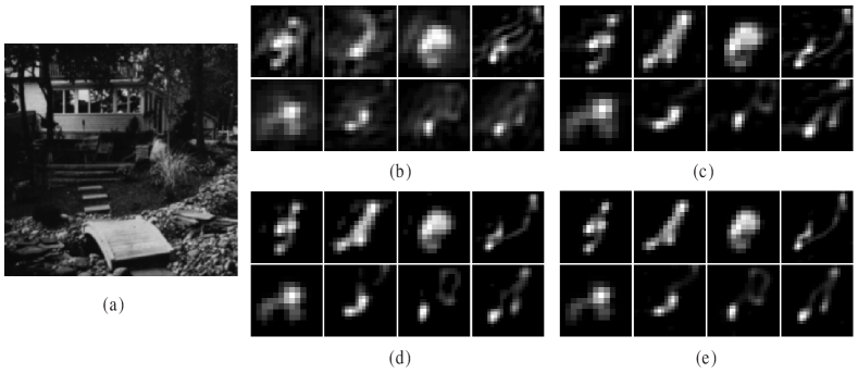
Fig. 7 shows an example that demonstrates the effectiveness of model (3) in the kernel estimation process. Due to the proposed structure selection mechanism, the kernel estimates (shown in Fig. 7 (e)) outperform those without adopting model (3) (i.e., Fig. 7 (b)). Compared with other structure selection methods [1, 3], our method outperforms better.

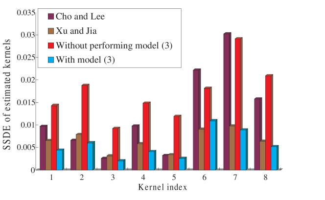
In Fig. 8, Sum of Squared Differences Error (SSDE) is employed to compare the estimation accuracy for the blur kernels in Fig. 7. One can see that the accuracy of kernel estimation by the proposed method has been greatly improved.

Figure 8: Comparison of kernel estimation results in terms of SSDE.

To further demonstrate the importance of salient edges $\nabla S$ and the effectiveness of our whole kernel estimation algorithm, we choose an example (i.e., the “im02_ker08” test case in the dataset in [11]) to conduct another experiment shown in Fig. 9.

Figure 9: Importance of salient edges $\nabla S$ and the effectiveness of our whole kernel estimation algorithm. The red curve shows the kernel estimation errors without adopting any structure selection strategies. The dashed green curve shows the kernel estimation errors without adopting model (3) in the proposed structure selection strategy. The cyan curve shows the kernel estimation errors with the proposed structure selection strategy. The dotted black curve shows the kernel estimation errors with the proposed structure selection strategy, while the salient edges are extracted from the ground truth image.

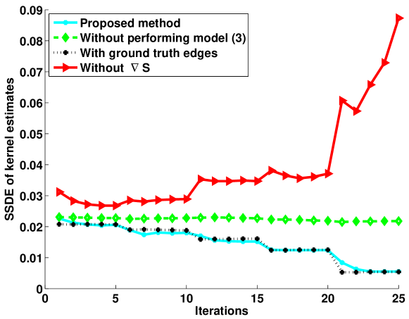
As we do not use salient edges $\nabla S$, the SSDE values of kernel estimates (i.e., the red curve in Fig. 9) are increasing with the iterations. In contrast, the results with $\nabla S$ (i.e., the cyan curve and the dashed green curve in Fig. 9) are better. This further demonstrates the importance of salient edges. Compared the cyan curve with the dashed green curve, the quality of kernel estimates that are generated by model (3) has been greatly improved. In addition, its accuracy and convergency are better than those without adopting model (3). This is also in line with our understanding (Illustrated in Section 1 and Section 3.1). From the cyan curve and the dotted black curve, one can see that our salient edges $\nabla S$ perform comparably to the salient edges that are extracted from the ground truth images. This further verifies the validity of our structure selection method.

3.5.2 Effectiveness of the Proposed Kernel Estimation Model

Although salient edges are very important, a robust kernel estimation model also plays a critical part in the kernel estimation process. Thus, we propose model (3.2) to estimate kernels. The results shown in Fig. 7 illustrate its effectiveness to some extent. The kernel estimates by [1, 3] contain some obvious noise and the continuity of some kernel estimates has also been destroyed. However, results shown in Fig. 7 (e) demonstrate that model (3.2) not only can remove noise but also preserve the continuity of the blur kernels.

To provide a more insightful illustration, we use the same dataset shown in Fig. 7(a) to demonstrate the effectiveness of our kernel estimation model.

Fig. 10 shows the comparison of kernel estimation results in terms of SSDE. Due to the influence of the constraint Eq. (11), the accuracy of estimated kernels is much higher.

Figure 10: The effectiveness of our kernel estimation model.

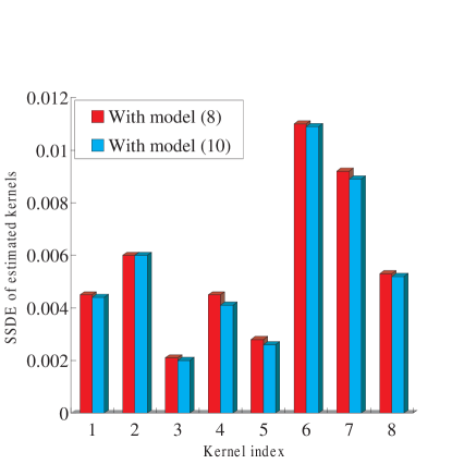
More illustrative examples are included in supplemental material.

4 Final Latent Image Estimation

Model (15) may lead to the stair-casing effect and destroy textures. To overcome this problem, some adaptive regularization terms have been proposed and proved to be effective in edge-preserving [31]. Inspired by this idea, we utilize our predicted structure to guide the latent image restoration. Our final model for latent image restoration is defined as

$$\min_{I}\|B-k*I\|_{2}^{2}+\lambda(\exp(-\|\partial_{x}S\|^{0.8})\|\partial_{x}I\|_{1}+\exp(-\|\partial_{y}S\|^{0.8})\|\partial_{y}I\|_{1}).$$ (16)

In model (16), the smoothness requirement is enforced in a spatially varying manner via the smoothness weights $\exp(-\|\partial_{x}S\|^{0.8})$ and $\exp(-\|\partial_{y}S\|^{0.8})$, which depend on the salient edges $\nabla S$. Hence, model (16) is able to contribute to the edge-preserving.

Model (16) can also be solved by the IRLS method efficiently. We run IRLS for 3 iterations. At each iterations, the weights for $\partial_{x}I$ and $\partial_{y}I$ are defined as

$$\left\{\begin{array}[]{ll}w_{x}=\frac{\exp(-|\partial_{x}S|^{0.8})}{\max\{|\partial_{x}I|,0.001\}},\\ w_{y}=\frac{\exp(-|\partial_{y}S|^{0.8})}{\max\{|\partial_{y}I|,0.001\}}.\end{array}\right.$$ (19)

We use 100 CG iterations in the inner IRLS system.

Based on above analysis, our deblurring algorithm is summarized in Alg. 3.

Algorithm 3 The Completed Image Deblurring Algorithm

  Input: Blur image $B$ and the size of blur kernel;

  Step 1: Estimate kernel $k$ by Alg. 2;

  Step 2: Estimate the final latent image $I$ according to model (16);

  Output: Latent image $I$.

5 Experiments

In this section, we present results of our algorithm and compare it to the state-of-the-art approaches of [4, 2, 1, 7, 3, 6]. We first introduce some implementation details. In the kernel estimation, all color images are converted to grayscale ones. The initialized value of $\theta$ is experimentally set to $1$ based on lots of experiments. The parameter $\lambda_{c}$ in model (15) is set to $0.005$, $\lambda$ in model (16) is set to $0.003$, and $\gamma$ in model (3.2) is set to $0.01$. In Alg. 1, solving model (14) will produce negative values. We project the estimated blur kernel onto the constraints (i.e., setting negative elements to 0 and renormalizing). In Alg. 2, we empirically set the inner iteration $m=5$. In the final deconvolution process, each color channel is separately processed.

5.1 Experimental Results and Evaluation

We first use a synthetic example shown in Fig. 11(a) to prove the effectiveness of our method. The blurred image contains rich textures and small details, such as flowers, leaves, and grass which increase the difficulty in kernel estimation. Methods of Fergus et al. [4] and Shan et al. [2] fail to provide correct kernel estimation results, and their deblurred results still contain some blur and ringing artifacts. Other methods [3, 1, 6] provide deblurred results with some ringing artifacts due to the imperfect kernel estimation results. However, our results shown in Fig. 11(g) perform well both in the kernel estimation and the final latent image restoration.

Figure 11: Small tiny details such as the grass and leaves are contained in the image. (a) Blurred image. (b) Result of Fergus et al. [4]. (c) Result of Shan et al. [2]. (d) Result of Cho and Lee [1]. (e) Result of Xu and Jia [3]. (f) Result of Krishnan et al. [6]. (g) Our result. (h) The ground truth result. The size of motion blur kernel is $27\times 27$.

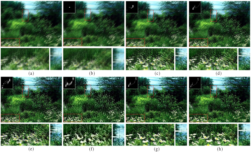
In Table 1, we employ SSDE and PSNR (Peak Signal to Noise Ratio) to compare the estimation accuracy for the blur kernels and the restored images in Fig. 11, respectively. Our method provides higher PSNR value for the restored image and lower SSDE value for the kernel estimate.

Table 1: Comparison of estimated results in Fig. 11.

Methods	[4]	[2]	[1]	[3]	[6]	Ours
PSNR of images	15.45	14.78	14.44	13.47	15.33	19.92
SSDE of kernels	0.2654	0.0329	0.0298	0.0301	0.0292	0.0021

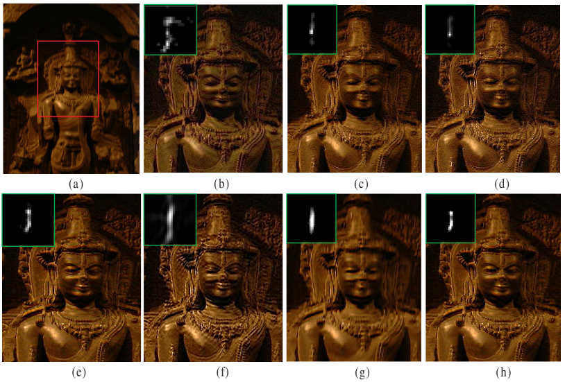
We then test the effectiveness of our structure selection model (3). Fig. 12(a) is a real captured image presented in [4]. The deblurred results of [4, 2, 1] contain some noise. The results of Xu and Jia [3] perform better, but the kernel estimate still contains some noise. Our method shown in Fig. 12(h) performs better in kernel estimation and latent image restoration. Fig. 12(g) shows our result without performing model (3). Compared to the result shown in Fig. 12(h), its quality is lower, indicating the importance of structures in estimating kernels.

Figure 12: Comparison of results with and without using image structures. (a) Blurred image. (b) - (h) are deblurred results cropped from the red box in (a). (b) Result of Fergus et al. [4]. (c) Result of Shan et al. [2]. (d) Result of Cho and Lee [1]. (e) Result of Xu and Jia [3]. (f) Result of Krishnan et al. [6]. (g) Result without performing model (3). (h) Result with model (3). The result (h) of our method is the best.

For real images with rich textures and small details, our method can still achieve good results. Fig. 13(a) shows a challenging example with tiny structures in the blurred image (published in [3]). The methods of Fergus et al. [4], Shan et al. [2], and Krishnan et al. [6] fail to provide the correct deblurred results and the kernel estimation results. The method of Cho and Lee [1] is able to estimate the blur kernel, but the deblurred contains some extra artifacts. The estimated kernel of Xu and Jia [3] is better, but the final deblurred result still contains some visual artifacts (shown in the red box in Fig. 13(e)). Moreover, the kernel estimation result contains some obvious noise (Fig. 13(j)). Our method outperforms these methods both in the kernel estimation and the latent image restoration. Compared with Fig. 13(g) and Fig. 13(h), our simple adaptive weighted spatial prior can preserve more sharp edges and finer textures in the latent image.

Figure 13: A challenging example with much tiny structures. These tiny structures greatly increase the difficulty of kernel estimation. (a) Blurred image. (b) Result of Fergus et al. [4]. (c) Result of Shan et al. [2]. (d) Result of Cho and Lee [1]. (e) Result of Xu and Jia [3]. (f) Result of Krishnan et al. [6]. (g) - (h): Our results. Deblurred results in (g) and (h) are generated by model (15) and (16), respectively. (i) Kernel estimate in [1]. (j) Kernel estimate in [3]. (k) Our kernel estimation result. The size of blur kernel is $45\times 45$.

Another important advantage of our method is that it can deal with large blur kernels. The photo in Fig. 14(a) is captured by ourselves, whose motion blur is quite large. The method of [1] performs better than that of [3], but the kernel estimation result still contains some noise, and the deblurred result is inaccurate in the red box. Due to the large blur, methods of [4, 2, 6] cannot produce correct kernel estimation results either and their deblurred results still contain some obvious blur and ringing artifacts (e.g., the part in the red boxes). Levin et al. [7]’s method provides better estimated results, but the estimated kernel still contains some noise and the deblurred result also contains some blur (e.g., the parts in the red boxes in Fig. 14(e)) Our approach, however, generates a better kernel estimate and the deblurred result is also visually comparable.

Figure 14: A large blur kernel estimation example. (a) Blurred image. (b) Result of Fergus et al. [4]. (c) Result of Shan et al. [2]. (d) Result of Cho and Lee [1]. (e) Result of Levin et al. [7]. (f) Result of Xu and Jia [3]. (g) Result of Krishnan et al. [6]. (h) Our result. The red boxes shown in (b) - (g) still contain some ringing artifacts or blur. Our estimated blur kernel size is $53\times 53$.

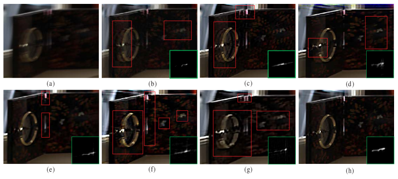
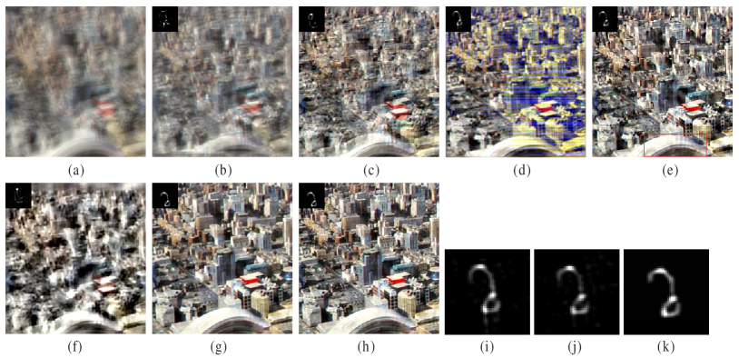
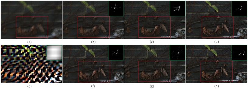
Fig. 15 shows another example with large motion blur. The blurred image (Fig. 15(a)) also contains small details. Due to the large blur, methods [4, 6, 7] cannot provide reasonable results. The deblurred result of [2] still contains some noise and ringing artifacts. Results of [1, 3] still contain some blur. Our method, however, provides a clearer image with finer textures.

Figure 15: Another large blur kernel estimation example. (a) Blurred image. (b) Result of Fergus et al. [4]. (c) Result of Shan et al. [2]. (d) Result of Cho and Lee [1]. (e) Result of Levin et al. [7]. (f) Result of Xu and Jia [3]. (g) Result of Krishnan et al. [6]. (h) Our result. Our estimated blur kernel size is $99\times 99$.

Evaluation on the Synthetic Dataset [11]: We perform quantitative evaluation of our kernel estimation method by using the dataset from Levin et al. [11], and compare our kernel estimation results with the state-of-the-art blind deblurring algorithms by Fergus et al. [4], Shan et al. [2], Cho and Lee [1], Xu and Jia [3], Krishnan et al. [6], and Levin et al.’s latest method [7]. For evaluation with each test case, we follow the method used in [11]. The kernel estimation results of [4, 2, 1, 3, 6, 7] are all generated by using the authors’ source codes or executable programs downloaded online. Then, the deblurred results are obtained by using Levin et al.’s [7] matlab function deconvSps.m with the same parameter settings. The error metric is also the same as [11] and it is defined as

$$\mathcal{E}=\frac{\|I_{r}-I_{g}\|_{2}^{2}}{\|I_{t}-I_{g}\|_{2}^{2}},$$ (20)

where $I_{r}$ and $I_{t}$ are the restored images with the estimated kernel and ground truth kernel, respectively, and $I_{g}$ is the ground truth image.

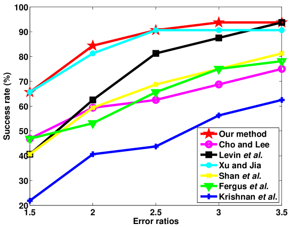
In Fig. 16, we plot the cumulative histograms of deconvolution error ratios in the same way as [7]. In the x-axis, a number of $n$ shows the percentage of test cases whose deconvolution error ratios are below $n$. Our method provides more reliable results than others.

Figure 16: Cumulative histogram of the deconvolution error ratio across test examples.

More comparison results can be found in our supplementary materials.

5.2 Computational Cost

In the kernel estimation process, we should iteratively solve models (3.2) and (15) which involve a few matrix-vector or convolution operations. For the computational time, our Matlab implementation spends about 2 minutes to estimate a $27\times 27$ kernel from a $255\times 255$ image with an Intel Xeon CPU@2.53GHz and 12GB RAM, while methods [4, 6, 7] need about 7 minutes, 3 minutes, and 4 minutes, respectively. The algorithm [2] implemented in C++ spends about 50 seconds. Compared with [1, 3], our method needs more computational time due to involving non-convex models in kernel estimation. However, in our kernel estimation process, both the kernel estimation step and latent image restoration step involve the CG method. Thus, we believe that our method is amenable to speedup with GPU acceleration by the strategy in [1].

5.3 Handling Blurred Images with Outliers

Outliers in the blurred image will increase the difficulty in kernel estimation and latent image restoration. Recent works [32, 33, 34] proposed robust non-blind deblurring methods to deal with outliers. When dealing with real blurred images with outliers, they used kernel estimation methods, e.g., [1, 3], to estimate blur kernels and then applied their methods to obtain a better deblurred result.

According to the strategies described in [32, 33, 34], our kernel estimation method can be applied to the images with outliers which distribute non-uniformly in the blurred image. Specifically, we use our kernel estimation method to estimate a blur kernel from an image patch without obvious outliers and then adopt the non-blind deblurring method [33] to restore the latent image. To demonstrate the effectiveness of our kernel estimation method, we choose an example from [35] and compare our method with [35], which is specialized on dealing with noise.

Figure 17: Blurred image with some noise. (a) Blurred image. (b) Result of [35]. (c) Our result. (d) The deblurred result is obtained by method [33], but the kernel is obtained by our method. The green boxes shown in (b) contain some ringing artifacts or blur.

From the results shown in Fig. 17, one can see that our estimated results are comparable with that of [35].

Fig. 18(a) shows a real blurred image with some saturated areas. Like the strategies [33, 34], we crop a rectangular region without obvious saturated pixels from Fig. 18(a) and estimate the blur kernel using the rectangular region (i.e., the part in the red box shown in Fig. 18(a)). We then use method [33] to restore the latent image.

Figure 18: Blurred image with some saturated areas. (a) Blurred image. (b) Our result. (c) The deblurred result is obtained by method [33], but the kernel is obtained by our method. The part shown in the red box in (a) is used to estimate the blur kernel.

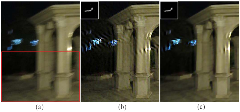
One can see that our method provides a reliable kernel. Due to the influence of saturated areas, the restored image shown in Fig. 18(b) contains some visual ringing artifacts.

These two examples, Figs. 17 and 18, further demonstrate the effectiveness of our kernel estimation method. However, it is noted that model (16) is not robust to outliers. The deblurred results shown in Figs. 17(c) and 18(b) demonstrate its limitations. Thus, developing a better non-blind method will be an interesting work.

6 Conclusion and Discussion

In this work, we developed a novel kernel estimation algorithm based on image salient edges. We discovered that image details could undermine the kernel estimation, especially for large blur kernels. Therefore, we proposed a self-adaptive algorithm which is able to remove structures with potential aversive effects to the estimation. Our kernel estimation model is able to remove noise and preserve the characteristics of the kernel, such as continuity and sparsity, which further reduces the aversive effects caused by the wrong chosen structures. In the final deconvolution step, we utilized the structural information for an adaptive weighted regularization term to guide the latent image restoration, which preserves the image details well.

We have extensively tested our algorithm, and found that it is able to deblur images with both small and large blur kernels especially when the blurred images contain rich details.

Our kernel estimation method would fail when the blurred image is textureless or contains severe saturated pixels. If the blurred image is textureless, we will not obtain salient edges for kernel estimation. If the blurred image contains a lot of saturated areas which distribute uniformly in the blurred image, these saturated areas will be chosen for kernel estimation due to their saliency. Since saturation breaks the linearity of the convolution-based blur model (1), this will inevitably damage the kernel estimation. In addition, a spatially varying blur would not be properly handled by our method. We leave these problems as our future work.

Appendix A Relationship to the Structure Extraction Method [36]

The work in [36] used local information to accomplish texture removal and they proposed a new adaptive regularization term named relative total variation (RTV) which is defined as

$$\mathfrak{R}_{x}(\textbf{x})=\frac{\sum_{\textbf{y}\in N_{h}(\textbf{x})}g_{\textbf{x},\textbf{y}}|\partial_{x}S(\textbf{y})|}{|\sum_{\textbf{y}\in N_{h}(\textbf{x})}g_{\textbf{x},\textbf{y}}\partial_{x}S(\textbf{y})|+\epsilon},$$

$$\mathfrak{R}_{y}(\textbf{x})=\frac{\sum_{\textbf{y}\in N_{h}(\textbf{x})}g_{\textbf{x},\textbf{y}}|\partial_{y}S(\textbf{y})|}{|\sum_{\textbf{y}\in N_{h}(\textbf{x})}g_{\textbf{x},\textbf{y}}\partial_{y}S(\textbf{y})|+\epsilon},$$ (21)

where $S$ is the structure that we want to get and $g_{\textbf{x},\textbf{y}}$ is a weighting function defined according to spatial affinity. If $g_{\textbf{x},\textbf{y}}$ is a scalar weight, then the effect of Eq. (A) is similar to that of $1/r(\textbf{x})$ or $w(\textbf{x})$. In fact, we can also use the variation form of Eq. (4), i.e.,

$$\mathfrak{R}(\textbf{x})=\frac{\sum_{\textbf{y}\in N_{h}(\textbf{x})}\|\nabla S(\textbf{y})\|}{\|\sum_{\textbf{y}\in N_{h}(\textbf{x})}\nabla S(\textbf{y})\|+\epsilon},$$

as a special regularizer to extract structures from an image. However, our structure extraction method is different from [36]. We use $w(\textbf{x})$ as an adaptive smoothness weight. Regarding the effect of RTV, we believe that it would extract some useful structures for kernel estimation.

References

- [1] S. Cho, S. Lee, Fast motion deblurring, ACM Transactions on Graphics (SIGGRAPH Asia) 28 (5) (2009) 145.
- [2] Q. Shan, J. Jia, A. Agarwala, High-quality motion deblurring from a single image, ACM Transactions on Graphics 27 (3) (2008) 73.
- [3] L. Xu, J. Jia, Two-phase kernel estimation for robust motion deblurring, in: ECCV, 2010, pp. 157–170.
- [4] R. Fergus, B. Singh, A. Hertzmann, S. T. Roweis, W. T. Freeman, Removing camera shake from a single photograph, ACM Transactions on Graphics 25 (3) (2006) 787–794.
- [5] N. Joshi, R. Szeliski, D. J. Kriegman, PSF estimation using sharp edge prediction, in: CVPR, 2008, pp. 1–8.
- [6] D. Krishnan, T. Tay, R. Fergus, Blind deconvolution using a normalized sparsity measure, in: CVPR, 2011, pp. 2657–2664.
- [7] A. Levin, Y. Weiss, F. Durand, W. T. Freeman, Efficient marginal likelihood optimization in blind deconvolution, in: CVPR, 2011, pp. 2657–2664.
- [8] W. G. Chen, N. Nandhakumar, W. N. Martin, Image motion estimation from motion smear-a new computational model, IEEE Transactions on Pattern Analysis Machine Intelligence 18 (1) (1996) 234–778.
- [9] T. Chan, C. Wong, Total variation blind deconvolution, IEEE Transactions on Image Processing 7 (3) (1998) 370–375.
- [10] J.-F. Cai, H. Ji, C. Liu, Z. Shen, Blind motion deblurring from a single image using sparse approximation, in: CVPR, 2009, pp. 104–111.
- [11] A. Levin, Y. Weiss, F. Durand, W. T. Freeman, Understanding and evaluating blind deconvolution algorithms, in: CVPR, 2009, pp. 1964–1971.
- [12] A. Goldstein, R. Fattal, Blur-kernel estimation from spectral irregularities, in: ECCV, 2012, pp. 622–635.
- [13] N. Joshi, Enhancing photographs using content-specific image priors, Ph.D. thesis, University of California (2008).
- [14] T. S. Cho, S. Paris, B. K. P. Horn, W. T. Freeman, Blur kernel estimation using the radon transform, in: CVPR, 2011, pp. 241–248.
- [15] Y. Wang, W. Yin, Compressed sensing via iterative support detection, Tech. rep., Rice CAAM Technical Report TR09-30 (2009).
- [16] Z. Hu, M.-H. Yang, Good regions to deblur, in: ECCV, 2012, pp. 59–72.
- [17] L. B. Lucy, An iterative technique for the rectification of observed distributions, Astronomy Journal 79 (6) (1974) 745–754.
- [18] L. Yuan, J. Sun, L. Quan, H.-Y. Shum, Progressive inter-scale and intra-scale non-blind image deconvolution, ACM Transactions on Graphics 27 (3) (2008) 74.
- [19] A. Levin, R. Fergus, F. Durand, W. T. Freeman, Image and depth from a conventional camera with a coded aperture, ACM Transactions on Graphics 26 (3) (2007) 70–78.
- [20] N. Joshi, C. L. Zitnick, R. Szeliski, D. J. Kriegman, Image deblurring and denoising using color priors, in: CVPR, 2009, pp. 1550–1557.
- [21] Y. Wang, J. Yang, W. Yin, Y. Zhang, A new alternating minimization algorithm for total variation image reconstruction, SIAM Journal on Imaging Sciences 1 (3) (2008) 248–272.
- [22] O. Whyte, J. Sivic, A. Zisserman, J. Ponce, Non-uniform deblurring for shaken images, in: CVPR, 2010, pp. 491–498.
- [23] N. Joshi, S. B. Kang, C. L. Zitnick, R. Szeliski, Image deblurring using inertial measurement sensors, ACM Transactions on Graphics 29 (4) (2010) 30.
- [24] A. Gupta, N. Joshi, C. L. Zitnick, M. F. Cohen, B. Curless, Single image deblurring using motion density functions, in: ECCV, 2010, pp. 171–184.
- [25] M. Hirsch, C. J. Schuler, S. Harmeling, B. Schölkopf, Fast removal of non-uniform camera shake, in: ICCV, 2011, pp. 463–470.
- [26] H. Ji, K. Wang, A two-stage approach to blind spatially-varying motion deblurring, in: CVPR, 2012, pp. 73–80.
- [27] L. I. Rudin, S. Osher, E. Fatemi, Nonlinear total variation based noise removal algorithms, Physica D 60 (1992) 259–268.
- [28] S. Osher, L. I. Rudin, Feature-oriented image enhancement using shock filters, SIAM Journal on Numerical Analysis 27 (4) (1990) 919–940.
- [29] J. Chen, L. Yuan, C. K. Tang, L. Quan, Robust dual motion deblurring, in: CVPR, 2008, pp. 1–8.
- [30] L. Xu, C. Lu, Y. Xu, J. Jia, Image smoothing via l gradient minimization, ACM Transactions on Graphics (SIGGRAPH Asia) 30 (6) (2011) 174.
- [31] Z. Farbman, R. Fattal, D. Lischinski, R. Szeliski, Edge-preserving decompositions for multi-scale tone and detail manipulation, ACM Transactions on Graphics 27 (3) (2008) 67.
- [32] H. Ji, K. Wang, Robust image deblurring with an inaccurate blur kernel, IEEE Transactions on Image Processing 21 (4) (2012) 1624–1634.
- [33] S. Cho, J. Wang, S. Lee, Handling outliers in non-blind image deconvolution, in: ICCV, 2011, pp. 495–502.
- [34] O. Whyte, J. Sivic, A. Zisserman, Deblurring shaken and partially saturated images, in: ICCV Workshops, 2011, pp. 745–752.
- [35] Y.-W. Tai, S. Lin, Motion-aware noise filtering for deblurring of noisy and blurry images, in: CVPR, 2012, pp. 17–24.
- [36] L. Xu, Q. Yan, Y. Xia, J. Jia, Structure extraction from texture via relative total variation, ACM Transactions on Graphics (SIGGRAPH Asia) 31 (6) (2012) 139.