Dynamical Eigenmodes of a Polymerized Membrane

Abstract

We study the bead-spring model for a polymerized phantom membrane in the overdamped limit, which is the two-dimensional generalization of the well-known Rouse model for polymers. We derive the exact eigenmodes of the membrane dynamics (the “Rouse modes”). This allows us to obtain exact analytical expressions for virtually any equilibrium or dynamical quantity for the membrane. As examples we determine the radius of gyration, the mean square displacement of a tagged bead, and the autocorrelation function of the difference vector between two tagged beads. Interestingly, even in the presence of tensile forces of any magnitude the Rouse modes remain the exact eigenmodes for the membrane. With stronger forces the membrane becomes essentially flat, and does not get the opportunity to intersect itself; in such a situation our analysis provides a useful and exactly soluble approach to the dynamics for a realistic model flat membrane under tension.

I Introduction

Bead-spring models for linear polymers, wherein the polymer is modelled as a sequence of beads connected by springs, play a central role in the theory of polymer dynamics. For a linear bead-spring polymer chain, with position ${\bf R}_{n}$ of the $n$-th bead, $n=1\dots N$, the potential energy is given by $\displaystyle{U=\frac{k}{2}\sum_{n=1}^{N-1}\left({\bf R}_{n}-{\bf R}_{n+1}\right)^{2}}$, in which $k$ is the spring constant. Within the scope of bead-spring models, the Rouse model rouse holds a special status, as it provides a framework for linear polymers by which virtually any static and dynamical quantity of interest can be calculated analytically doi ; de . In the Rouse model the dynamics of the beads is formulated in the overdamped limit. For solving the Rouse model one considers the so-called Rouse modes (rather than the equations of motion for the individual beads). Using the mode amplitude correlation functions, the quantities of interest for a phantom chain can be analytically tracked by reconstructing them from the modes doi ; de . The Rouse model has been shown useful for self-avoiding linear polymers chain1 , and to show that the dynamics of a tagged bead in a linear bead-spring model is described by the Generalized Langevin Equation (GLE) jstat1 ; jstat2 .

It is therefore a natural question to ask if the analytical solution of the Rouse model can be generalized to higher dimensions, e.g., making it useful for the dynamics of polymerized membranes. There is a considerable amount interest in the properties of polymerized membranes book . The interest stems not only from the point of view of a fundamental understanding, but also because of their importance in biology and chemistry. Instances of polymerized membranes with a fixed connectivity can be found in 2D-cytoskeletons of cells cells1 ; cells2 ; cells3 and graphite oxide sheets sheet1 ; sheet2 ; sheet3 .

Static properties of polymerized membranes as a two-dimensional extension of (one-dimensional) linear polymers came into fashion in the late 80s. At that time the driving question centered on the equilibrium properties of polymerized membranes, in particular, the scaling of the radius of gyration of a polymerized membrane with its lateral size, while the corresponding scaling behavior for phantom and self-avoiding linear polymers were already well-known. Sophisticated renormalized group approaches were developed to this end renorm1 ; renorm2 ; renorm3 ; renorm4 , accompanied by computer simulations mcsim1 ; mcsim2 ; mcsim3 ; mcsim4 ; mcsim5 ; mcsim6 ; mcsim7 ; mcsim8 ; mcsim9 . A notable outcome of these studies is that the radius of gyration $R_{g}$ of a membrane scales with its lateral size $N$ as $R_{g}\sim\log N$ for phantom, and as $R_{g}\sim N$ for self-avoiding membranes.

In contrast to the equilibrium properties, the dynamical properties of membranes have been studied with less intensity. Apart from scaling analyses dynamana1 ; dynamana2 ; dynamana3 , the bulk of the research on the dynamics of polymerized membranes are heavily dominated by computer simulations dynammcsim1 ; dynammcsim2 ; dynammcsim3 ; dynammcsim4 , leaving exact analytical results on the dynamics of membranes a relatively open area. In this paper we attempt to fill this void — we consider two-dimensional square-polymerized phantom membranes embedded in a three-dimensional space, both in the absence and the presence of tensile forces — and perform a Rouse mode analysis. We show that the Rouse modes are the exact eigenmodes of the membrane dynamics. Akin to the Rouse model for bead-spring linear polymers, our exercise allows us to exactly solve for the static and dynamic properties of phantom membranes; in this process also deriving the exact expression for the scaling of $R_{g}$ as a function of the membrane’s lateral size $N$ (which confirms the $R_{g}\sim\log N$ scaling), as well as show increased fluctuations at the edge of the membrane edge1 ; edge2 . In particular, we draw the reader’s attention to the exact solution under tensile forces, for which forces the membrane essentially encounters a flat geometry. Unlike a phantom membrane in equilibrium, in such a situation the membrane becomes essentially flat, does not get the opportunity to intersect itself, and therefore provides a highly useful and exactly soluble approach to the dynamics for a realistic model flat membrane. We also note that the methods are generalizable to arbitrary internal and spatial dimensions.

The structure of this paper is as follows. In Sec. II we describe the dynamical equations without forces, and their diagonalization by the Rouse modes. In Sec. III we derive the scaling of the radius of gyration, the mean-square displacement of a tagged bead and the autocorrelation function of a vector connecting two beads. In Sec. IV we incorporate tensile forces in the dynamical equations and derive the new Rouse modes that diagonalize them. We finally end the paper with a discussion in Sec. V.

II Diagonalization of equations of motion for the polymerized membrane and the Rouse modes

We consider a rectangular polymerized membrane, for which $N=L_{1}\times L_{2}$ beads are connected in a perpendicular toplogy, with ${\bf R}_{{\bf n}}(t)$ denoting the spacial position at time $t$ of the bead internally labeled as ${\bf n}$. Naturally for a membrane it is convenient to take two numbers ${\bf n}=(n_{1},n_{2})$ for labeling the beads with $n_{i}=1,\dots,L_{i}$. The potential energy for a square-polymerized membrane is a simple extension of the Hamiltonian for a linear polymer in two internal dimensions

$$U=\frac{k}{2}\sum_{n_{1},n_{2}=1}^{L_{1}-1,L_{2}}\left({\bf R}_{n_{1},n_{2}}-{\bf R}_{n_{1}+1,n_{2}}\right)^{2}+\frac{k}{2}\sum_{n_{1},n_{2}=1}^{L_{1},L_{2}-1}\left({\bf R}_{n_{1},n_{2}}-{\bf R}_{n_{1},n_{2}+1}\right)^{2}$$ (1)

for some spring constant $k$.

In the absence of externally applied forces, in the overdamped limit the dynamics of each bead of the membrane is described by

$$\frac{d{\bf R}_{{\bf n}}}{dt}=-\frac{1}{\zeta}\frac{\partial U}{\partial{\bf R}_{{\bf n}}}+{\bf g}_{{\bf n}},$$ (2)

where $\zeta$ is the friction coefficient of the solvent and ${\bf g}_{{\bf n}}$ is the thermal force on the ${\bf n}$-th bead. The thermal forces are uncorrelated between different beads, as well as in time, i.e.,

$$\left<{\bf g}_{{\bf m}}(t)\cdot{\bf g}_{{\bf n}}(t^{\prime})\right>=\frac{6k_{B}T}{\zeta}\delta_{{\bf m}{\bf n}}\delta(t-t^{\prime}),$$ (3)

with Boltzmann constant $k_{B}$ and temperature $T$.

For a linear polymer with positions ${\bf R}_{n}(t)$ of beads $n=1,\dots,N$ at time $t$ the Rouse modes are given by doi ; de

$${\bf X}_{p}(t)=\frac{1}{N}\sum_{n=1}^{N}\cos\left[\frac{\pi(n-1/2)p}{N}\right]{\bf R}_{n}(t),$$ (4)

with $p=0,\dots,N-1$ and the inverse given by

$${\bf R}_{n}(t)={\bf X}_{0}(t)+2\sum_{p=1}^{N-1}\cos\left[\frac{\pi(n-1/2)p}{N}\right]{\bf X}_{p}(t)$$ (5)

The Rouse modes for the membrane are quite similar to those of the linear chain: since topologically the internal directions (connectivity) are orthogonal, the Rouse modes will be products of Rouse modes for a linear polymer. Below we introduce the following definitions for an elegant notation and proof of the independence of the Rouse modes.

First we define

$$\beta_{p_{i}}=\left\{\begin{array}[]{ll}2&\mbox{if }p_{i}=1,\dots,L_{i}-1\\ 1&\mbox{if }p_{i}=0\end{array}\right.,\quad\beta_{{\bf p}}=\beta_{p_{1}}\beta_{p_{2}}$$ (6)

and

$$f_{p_{i}}(n_{i})=\cos\left[\frac{\pi p_{i}(n_{i}-1/2)}{L_{i}}\right],\quad f_{{\bf p}}({\bf n})=f_{p_{1}}(n_{1})f_{p_{2}}(n_{2})$$ (7)

The orthogonality relation at the basis of the proof for the Rouse modes for a linear polymer chain can then be generalized for the membrane

$$\frac{1}{N}\sum_{{\bf n}}\beta_{{\bf p}}f_{{\bf p}}({\bf n})f_{{\bf q}}({\bf n})=\delta_{{\bf p}{\bf q}},$$ (8)

where the summation is taken over all allowed values of ${\bf n}$. The Rouse modes amplitudes and the corresponding inverse are then given by

$${\bf X}_{{\bf p}}(t)=\frac{1}{N}\sum_{{\bf n}}f_{{\bf p}}({\bf n}){\bf R}_{{\bf n}}(t),$$ (9)

$${\bf R}_{{\bf n}}(t)=\sum_{{\bf p}}\beta_{{\bf p}}f_{{\bf p}}({\bf n}){\bf X}_{{\bf p}}(t).$$ (10)

The position of the center-of-mass ${\bf R}_{\text{cm}}(t)$ at time $t$ simply equals ${\bf X}_{{\bf 0}}(t)$.

Next, we note that when the equations of motion from Eq. (2) for the beads are expressed one gets a term for each internal dimension equal to that of a term for a bead in a linear polymer. Taking the time derivative in Eq. (9) and plugging in the equations of motion for the beads and then the inverse we get

$$\frac{d{\bf X}_{{\bf p}}(t)}{dt}=-\alpha_{{\bf p}}{\bf X}_{{\bf p}}(t)+{\bf G}_{{\bf p}}(t)$$ (11)

$$\mbox{ with }\alpha_{{\bf p}}\equiv 4\frac{k}{\zeta}\left(\sin^{2}\left[\frac{\pi p_{1}}{2L_{1}}\right]+\sin^{2}\left[\frac{\pi p_{2}}{2L_{2}}\right]\right)\mbox{ and }{\bf G}_{{\bf p}}(t)=\frac{1}{N}\sum_{{\bf n}}f_{{\bf p}}({\bf n}){\bf g}_{{\bf n}}(t),$$ (12)

i.e., the Rouse modes diagonalizes the equations of motion. This set of linearized differential equations can be solved just as for a linear polymer by using the correlation function for the thermal forces given by Eq. (3). By using the orthogonality relation in Eq. (8)

$$\left<{\bf G}_{{\bf p}}(t)\cdot{\bf G}_{{\bf q}}(t^{\prime})\right>=\frac{6k_{B}T}{\zeta N\beta_{{\bf p}}}\delta_{{\bf p}{\bf q}}\delta(t-t^{\prime}),$$ (13)

so that the following two-point correlation functions for the eigenmodes can be derived:

$$X_{\bf 00}(t)\equiv\langle[{\bf X}_{{\bf 0}}(t)-{\bf X}_{{\bf 0}}(0)]^{2}\rangle\equiv\langle[{\bf R}_{\text{cm}}(t)-{\bf R}_{\text{cm}}(0)]^{2}\rangle=\frac{6k_{B}T}{\zeta N}t$$ (14)

$$X_{{\bf p}{\bf q}}(t)\equiv\langle{\bf X}_{{\bf p}}(t)\cdot{\bf X}_{{\bf q}}(0)\rangle=\frac{3k_{B}T}{\zeta N\beta_{{\bf p}}}\frac{1}{\alpha_{{\bf p}}}\exp\left[-\alpha_{{\bf p}}t\right]\delta_{{\bf p}{\bf q}}\quad\mbox{with }{\bf p}\neq{\bf 0}.$$ (15)

Just like the case of a linear polymer, any correlation function of interest for the membrane can be derived using Eqs. (11-13). We address a few of them in the following section.

III A few properties of interest for a membrane

All throughout this section, for the sake of simplicity, we restrict ourselves to square membranes with $L_{1}=L_{2}=L$, and thus $N=L\times L$.

III.1 Scaling of the radius of gyration $R_{g}$

The radius of gyration squared for the membrane is defined by

$$R^{2}_{g}\equiv \frac{1}{N}\sum_{{\bf n}}\left\langle\left[{\bf R}_{{\bf n}}(t)-{\bf R}_{\text{cm}}(t)\right]^{2}\right\rangle$$

$$= \frac{1}{N}\sum_{{\bf n}}\sum_{{\bf p}\neq{\bf 0}}\sum_{{\bf q}\neq{\bf 0}}\langle{\bf X}_{{\bf p}}(t)\cdot{\bf X}_{{\bf q}}(t)\rangle\beta_{{\bf p}}\beta_{{\bf q}}f_{{\bf p}}({\bf n})f_{{\bf q}}({\bf n}),$$ (16)

in which Eq. (10) is used for the second line. Having plugged in Eqs. (8) and (15) the squared radius of gyration reduces to

$$R^{2}_{g}=\frac{3k_{B}T}{\zeta N}\sum_{{\bf p}\neq{\bf 0}}\frac{1}{\alpha_{{\bf p}}}.$$ (17)

The summation (17), using the definition of $\alpha_{\bf p}$ (12), can be split into two parts:

$$R^{2}_{g}=\frac{k_{B}T}{k}\left(\frac{3}{2N}\sum_{p=1}^{L-1}\sin^{-2}\left[\frac{\pi p}{2L}\right]+\frac{3k}{\zeta N}\sum_{p_{1}=1}^{L-1}\sum_{p_{2}=1}^{L-1}\frac{1}{\alpha_{{\bf p}}}\right)=\frac{k_{B}T}{k}\left(\mathcal{I}+\mathcal{J}\right).$$ (18)

The first term in Eq. (18) can be evaluated exactly: $\mathcal{I}=(N-1)/N$. For the second term we take the long polymer limit $N\gg 1$ so that $\alpha_{{\bf p}}$ can be expanded and the sum approximated by an integral with $x_{i}=p_{i}/L$ where the integral is over a unit square in the positive quadrant excluding the small area near the origin. The second approximation we make is replacing the area of integration by that of the positive quadrant of a unit circle excluding the small area near the origin which can be solved analytically

$$\mathcal{J}=\frac{3}{\pi^{2}}\int\frac{d{\bf x}}{x^{2}}=\frac{3}{2\pi}\int_{1/L}^{1}\frac{dr}{r}=\frac{3}{4\pi}\log N.$$ (19)

The radius of gyration squared for a square membrane in the long polymer limit thus becomes

$$R^{2}_{g}=\frac{k_{B}T}{k}\left(\frac{N-1}{N}+\frac{3}{4\pi}\log N\right).$$ (20)

A comparison between the two terms in Eq. (20) shows that the second one is bigger than the first one for $N>61$. In Fig. 1 we present a comparison between the analytical result (20) and the exact evaluation of Eq. (17) for $L$ up to $L=10^{4}$. Our result (20) confirms the $\log N$ scaling of $R_{g}^{2}$ obtained earlier by field-theory methodsrenorm1 ; renorm2 ; renorm3 ; renorm4 .

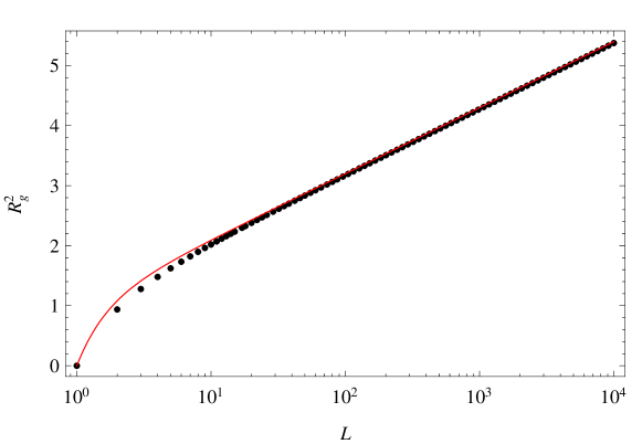
Figure 1: The radius of gyration squared $R_{g}^{2}$ for a square membrane as a function of $N=L\times L$ beads, with $k_{B}T/k$ set to unity. The black dots represents the sum in Eq. (17) evaluated exactly for $L$ up to $L=10^{4}$, while the continuous red line represents the function $(N-1)/N+3/(4\pi)\log N$.

III.2 Mean-square displacement of a tagged bead

Let us define $\Delta{\bf R}_{{\bf n}}(t)\equiv{\bf R}_{{\bf n}}(t)-{\bf R}_{{\bf n}}(0)$ for the ${\bf n}$-th bead. We use Eq. (10) to write

$$\langle\Delta{\bf R}_{{\bf n}}(t)^{2}\rangle= \langle[{\bf X}_{{\bf 0}}(t)-{\bf X}_{{\bf 0}}(0)]^{2}\rangle$$

$$+2\sum_{{\bf p}\neq{\bf 0}}\sum_{{\bf q}\neq{\bf 0}}\beta_{{\bf p}}\beta_{{\bf q}}f_{{\bf p}}({\bf n})f_{{\bf q}}({\bf n})\left\{X_{{\bf p}{\bf q}}(0)-X_{{\bf p}{\bf q}}(t)\right\}.$$ (21)

Using Eqs. (14-15) this simplifies to

$$\langle\Delta{\bf R}_{{\bf n}}(t)^{2}\rangle=\frac{6k_{B}T}{\zeta N}t+\frac{6k_{B}T}{\zeta N}\sum_{{\bf p}\neq{\bf 0}}\frac{\beta_{{\bf p}}}{\alpha_{{\bf p}}}f_{{\bf p}}({\bf n})^{2}\left\{1-e^{-\alpha_{{\bf p}}t}\right\}.$$ (22)

At short times $kt/\zeta\ll 1/8$ the exponential in the second term can be expanded, and the sum is exactly evaluated. In comparison to the second term the first one can be neglected to obtain

$$\langle\Delta{\bf R}_{{\bf n}}(t)^{2}\rangle=\frac{6k_{B}T}{\zeta}t\frac{1}{N}\sum_{{\bf p}\neq{\bf 0}}\beta_{{\bf p}}f_{{\bf p}}({\bf n})^{2}=\frac{6k_{B}T}{\zeta}t,$$ (23)

which agrees with the mean-square displacement of a free bead, and confirms the wisdom that at short times the beads do not feel the connectivity.

At very long times the exponentials in Eq. (22) reduce to zero, the second term becomes a fixed number independent of $t$ [but dependent on the location of the bead: the sum is largest when the bead is located at the corner of the membrane, and equals $6k_{B}T\left(\log N/\pi-\pi/4+2/3\right)/k$]; i.e., for $kt/\zeta\gg N\log N/\pi$ the first term of Eq. (21) dominates, and the motion of the tagged bead becomes simply diffusive, with the same diffusion coefficient as that of the center-of-mass.

At intermediate times the mean-square displacement of the tagged bead will depend on its location on the membrane. We work out three difference cases when the tagged bead is (a) the central bead of the membrane, (b) located in the middle of an edge, and (c) a corner bead. The enhanced mobility of edge and corner beads was already reported for self-avoiding membranes edge1 ; edge2 .

(a) For the mean-square displacement of a bead at the center of the membrane $\langle\Delta{\bf R}_{\text{m}}(t)^{2}\rangle$ the sum in Eq. (22) will only be over even values of $p_{i}$. In the long polymer limit the sum can be converted to an integral with $x_{i}=p_{i}/L$, such that

$$\langle\Delta{\bf R}_{\text{m}}(t)^{2}\rangle=\frac{6k_{B}T}{\zeta}\int_{0}^{1}dx_{1}\int_{0}^{1}dx_{2}\frac{1}{\alpha_{{\bf p}}}\left\{1-e^{-\alpha_{{\bf p}}t}\right\}=\frac{6k_{B}T}{\zeta}\int_{0}^{t}dt^{\prime}\int_{0}^{1}dx_{1}\int_{0}^{1}dx_{2}e^{-\alpha_{{\bf p}}t^{\prime}}.$$ (24)

We proceed with Eq. (24) by splitting the exponentials, resulting in two identical integrals which can be evaluated in terms of the modified Bessel function of the first kind $I_{\alpha}(z)$ and making a change of variables.

$$\langle\Delta{\bf R}_{\text{m}}(t)^{2}\rangle=\frac{6k_{B}T}{\zeta}\int_{0}^{t}dt^{\prime}\left(\int_{0}^{1}dx\exp\left\{-\frac{4kt^{\prime}}{\zeta}\sin^{2}\left[\frac{\pi}{2}x\right]\right\}\right)^{2}=\frac{6k_{B}T}{k}\int_{0}^{\frac{kt}{\zeta}}dt^{\prime}e^{-4t^{\prime}}I_{0}^{2}(2t^{\prime}).$$ (25)

To characterize the moderate time behavior of Eq. (25) we look at the asymptotic expansion $I_{\alpha}(z)=\exp(z)/\sqrt{2\pi z}$ and evaluated the integral so that

$$\langle\Delta{\bf R}_{\text{m}}(t)^{2}\rangle=\frac{3k_{B}T}{2\pi k}\left(\log\left[\frac{kt}{\zeta}\right]+C_{\text{m}}\right),$$ (26)

where

$$C_{\text{m}}=\lim_{x\rightarrow\infty}-\log[x]+4\pi\int_{0}^{x}dte^{-4t}I_{0}^{2}(2t)\approx 4.04.$$ (27)

(b-c) The same can be done for the mean-square displacement for a bead located in the middle of an edge $\langle\Delta{\bf R}_{\text{e}}(t)^{2}\rangle$ and corner $\langle\Delta{\bf R}_{\text{c}}(t)^{2}\rangle$. The corresponding calculations are similar to those in (a), and they yield

$$\langle\Delta{\bf R}_{\text{e}}(t)^{2}\rangle=\frac{3k_{B}T}{\pi k}\left(\log\left[\frac{kt}{\zeta}\right]+C_{\text{e}}\right),$$ (28)

where

$$C_{\text{e}}=\lim_{x\rightarrow\infty}-\log[x]+2\pi\int_{0}^{x}dte^{-4t}\left(I_{0}(2t)+I_{1}(2t)\right)I_{0}(2t)\approx 2.47,$$ (29)

and

$$\langle\Delta{\bf R}_{\text{c}}(t)^{2}\rangle=\frac{6k_{B}T}{\pi k}\left(\log\left[\frac{kt}{\zeta}\right]+C_{\text{c}}\right),$$ (30)

where

$$C_{\text{c}}=\lim_{x\rightarrow\infty}-\log[x]+\pi\int_{0}^{x}dte^{-4t}\left(I_{0}(2t)+I_{1}(2t)\right)^{2}\approx 1.47.$$ (31)

Figure 2: The mean-squared displacement $\langle\Delta{\bf R}_{{\bf n}}(t)^{2}\rangle$ for beads in a square membrane as a function of scaled time $kt/\zeta$. The sum in Eq. (22) was exactly evaluated for $k_{B}T/k=1$ for beads at the center of the membrane, at the middle of an edge, and at a corner for $N=301^{2}$ and the result is represented by the circular (red), triangular (green), and square (blue) data points respectively. The cyan diamonds represent the exact evaluation for a bead with internal position ${\bf n}=(151,5)$ to show the transition that the mean-squared displacement for a bead makes from one region to another. For very short times $kt/\zeta\ll 1/8$ the mean-squared displacement for all beads $\langle\Delta{\bf R}_{{\bf n}}(t)^{2}\rangle\sim t$ thus behaving like that of a free bead as shown in Eq. (23) which is represented by the dashed line in (a). For very long times the mean-squared displacement for all beads $\langle\Delta{\bf R}_{{\bf n}}(t)^{2}\rangle\sim t/N$ behaves like that of a mean-squared displacement of the center-of-mass which is represented by the dotted line in (a). In the intermediate time regime the mean-square displacement for beads $\langle\Delta{\bf R}_{{\bf n}}(t)^{2}\rangle\sim\log[kt/\zeta]$ as in agreement with Eqs. (26), (28) and (30) — the corresponding approximations are valid for $kt/\zeta\ll N/\pi^{2}$ — and are represented by the red, green, and blue solid lines in (b) respectively.

Note that all constants $C$’s can be evaluated up to arbitrary precision, and that that the approximations (25), (27) and (29) are valid for $kt/\zeta\ll N/\pi^{2}$. In Fig. 2 we compare the exact evaluations from Eq. (22) and the corresponding approximations (23), (26), (28) and (30).

III.3 Autocorrelation function of a vector connecting two beads

In the most general case the vector ${\bf r}_{{\bf m}{\bf n}}(t)\equiv{\bf R}_{{\bf m}}(t)-{\bf R}_{{\bf n}}(t)$ connects two beads with internal coordinates ${\bf m}$ and ${\bf n}$ at time $t$. The autocorrelation function of this vector $D_{{\bf m}{\bf n}}(t)\equiv\langle{\bf r}_{{\bf m}{\bf n}}(t)\cdot{\bf r}_{{\bf m}{\bf n}}(0)\rangle$ can be expressed in terms of the eigenmodes

$$D_{{\bf m}{\bf n}}(t)=\frac{3k_{B}T}{\zeta N}\sum_{{\bf p}\neq{\bf 0}}\frac{\beta_{{\bf p}}}{\alpha_{{\bf p}}}\left[f_{{\bf p}}({\bf m})-f_{{\bf p}}({\bf n})\right]^{2}\exp\left[-\alpha_{{\bf p}}t\right].$$ (32)

Like in the case for the mean-square displacement of a tagged bead, the behavior of $D_{{\bf m}{\bf n}}(t)$ depends on time and the internal positions of the beads, hence we only briefly outline the calculation procedure and state the results. We focus on two extreme cases (a) $D_{\text{c}}(t)$ where the vector connecting the two beads located at the opposite corners of the membrane, and (b) $D_{\text{a}}(t)$ where the vector connects two beads at position ${\bf n}$ and ${\bf n}+{\bf a}$ somewhere in the middle of the membrane for $a/L\equiv|{\bf a}|/L\ll 1$. We will generalize these results qualitatively for the cases when the locations of the beads and the distances between them are arbitrary.

Short times: For times $kt/\zeta\ll 1/8$ the exponent is roughly $1$ and so the functions are constant. In case two beads are close neighbors the sum can be evaluated $D_{\text{a}}(t)=k_{B}T(3/2+\log a)/k$, which is exact for $a=1$, and a rough estimate $D_{\text{c}}(t)=6k_{B}T\log N/(\pi k)$ follows from a calculation similar to that performed for the radius of gyration.

Figure 3: The scaled autocorrelation function $D_{{\bf m}{\bf n}}(t)/D_{{\bf m}{\bf n}}(0)$ of the vector connecting beads with internal position ${\bf m}$ and ${\bf n}$ in a square membrane as a function of scaled time $kt/\zeta$. The sum in Eq. (32) was exactly evaluated with $k_{B}T/k=1$ for two beads at positions [(251,251),(250,251)], [(251,254),(258,251)], [(1,1),(501,501)], and [(251,281),(281,251)] in the membrane with $N=501^{2}$, with the results shown by the circular (red), triangular (green), square (blue), and diamond (cyan) data points respectively. Note that the first two pairs of beads are very close to each other in the middle of the membrane where the third pair are two beads in opposing corners of the membrane; i.e., the first two cases correspond to $D_{\text{a}}(t)/D_{\text{a}}(0)$, while the third one corresponds to $D_{\text{c}}(t)/D_{\text{c}}(0)$. The function $D(t)\sim\log[kt/\zeta]$, as in agreement with Eq. (34) corresponding to the blue solid line in (b), for a duration that is larger when the beads are connected by a larger vector ${\bf a}$. For very small vectors ${\bf a}$ the behavior will shift to $D(t)\sim 1/t$ as derived in Eq. (33) corresponding to the red and green solid lines in (a) before $kt/\zeta\sim N/\pi^{2}$. The function $D(t)$ for the last pair shows a transition from logarithmic behavior to $D(t)\sim 1/t$ before the diffusive time regime.

Intermediate times: For $a/L\ll 1$ the sum for $D_{\text{a}}(t)$ can be expanded in $a$ and evaluated as

$$D_{\text{a}}(t)=\frac{3\zeta k_{B}T}{8\pi k^{2}}\frac{a^{2}}{t}.$$ (33)

Further, it can be shown that the summation for $D_{\text{c}}(t)$ equals that of $-\langle\Delta{\bf R}_{\text{c}}(t)^{2}\rangle$ up to a constant, such that

$$D_{\text{c}}(t)=D_{\text{c}}(0)-\frac{6k_{B}T}{\pi k}\left(\log\left[\frac{kt}{\zeta}\right]+C_{\text{c}}\right).$$ (34)

Long times: For $a/L\ll 1$ and $kt/\zeta\gg N/\pi^{2}$ only the lowest mode contributes to the summation and so expanding the correlation function in Eq. (32) yields

$$D_{\text{a}}(t)=\frac{6k_{B}Ta^{2}}{kN}\exp\left[-\frac{\pi^{2}k}{\zeta N}t\right],$$ (35)

while

$$D_{\text{c}}(t)=\frac{48k_{B}T}{\pi^{2}k}\exp\left[-\frac{\pi^{2}k}{\zeta N}t\right].$$ (36)

It is interesting to note the differences in behavior for $D_{\text{a}}(t)$ and $D_{\text{c}}(t)$ at intermediate times. The reason behind this difference is as follows. For $D_{\text{a}}(t)$ the beads are close and as a result they quickly become ‘aware’ of each other’s presence. For $D_{\text{c}}(t)$ on the other hand, the beads do not become ‘aware’ of each other’s presence almost until $kt/\zeta\sim N/\pi^{2}$. Based on this observation we expect that when the beads are neither very close nor very far, there will be first a logarithmic decay (34) for $D_{{\bf m}{\bf n}}(t)$, followed by a $1/t$ power-law decay (33) before the terminal exponential decay (35-36) sets in. The above results are verified by comparing the approximations to the exact evaluation of Eq. (32) for different pairs of beads in Fig. 3.

IV Dynamical eigenmodes in the case of external tensile forces

In this section we concentrate on presenting the exact eigenmodes when the membrane is stretched in two perpendicular directions by forces ${\bf F}_{1}$ and ${\bf F}_{2}$ applied at the edges of the membrane.

Adding tensile forces to the system ensures that each bead has its own mean position around which it fluctuates due to thermal forces. For large enough tensile forces the beads are far enough away from each other, and self-intersection of the membrane is avoided. Such a situation therefore mimics the behavior of a realistic flexible membrane under tension. The system is still exactly solvable by introducing the following term to the Hamiltonian

$$U_{F}=\sum_{n_{1},n_{2}=1}^{L_{1}-1,L_{2}}{\bf F}_{1}\cdot\left({\bf R}_{n_{1},n_{2}}-{\bf R}_{n_{1}+1,n_{2}}\right)+\sum_{n_{1},n_{2}=1}^{L_{1},L_{2}-1}{\bf F}_{2}\cdot\left({\bf R}_{n_{1},n_{2}}-{\bf R}_{n_{1},n_{2}+1}\right),$$ (37)

making the exercise of this section useful for practical purposes.

The mode amplitudes and their inverses are once again defined by Eqs. (9-10), but the following term ${\bf H}_{{\bf p}}$ will be added to the right hand side of the differential equation in Eq. (11) in order to solve for the dynamics of the mode amplitudes:

$${\bf H}_{{\bf p}} = \frac{1}{\zeta N}\sum_{{\bf n}}f_{{\bf p}}({\bf n})\left[{\bf F}_{1}(\delta_{n_{1}L_{1}}-\delta_{n_{1}1})+{\bf F}_{2}(\delta_{n_{2}L_{2}}-\delta_{n_{2}1})\right]$$ (38)

$$= \frac{1}{\zeta}\left[\delta_{p_{2}0}\{f_{p_{1}}(L_{1})-f_{p_{1}}(1)\}\frac{{\bf F}_{1}}{L_{1}}+\delta_{p_{1}0}\{f_{p_{2}}(L_{2})-f_{p_{2}}(1)\}\frac{{\bf F}_{2}}{L_{2}}\right].$$

Note that spatial symmetry for the modes is broken, and that Eq. (15) is replaced by similar equations but also depending on the spatial components $i$ and $j$ of the vectors.

$$X_{{\bf p}i{\bf q}j}(t)\equiv\langle{\bf X}_{{\bf p}i}(t){\bf X}_{{\bf q}j}(0)\rangle=\frac{{\bf H}_{{\bf p}i}{\bf H}_{{\bf q}j}}{\alpha^{2}_{{\bf p}}}+\frac{k_{B}T}{\zeta N\beta_{{\bf p}}}\frac{1}{\alpha_{{\bf p}}}\exp\left[-\alpha_{{\bf p}}t\right]\delta_{{\bf p}{\bf q}}\delta_{ij}\quad\mbox{with }{\bf p}\neq{\bf 0}.$$ (39)

The assumption ${\bf F}_{1}\perp{\bf F}_{2}$ is necessary in order for the modes to be the exact dynamical eigenmodes. If the tensile forces are not orthogonal, then it will result in correlations between some of the modes (and correspondingly a parallelogram-like structure of the membrane).

Figure 4: A randomly generated membrane consisting of $25\times 25$ beads in a three dimensional space, with orthonormal tensile forces, $k_{B}T=1/2$, and $k=\zeta=1$. The black lines connects neighboring beads. Due to tensile forces the membrane gets a rectangular lattice like structure where thermal forces push the beads out of their mean positions.

It is of course interesting to investigate the transverse fluctuations of the membrane under lateral tension. Two observables we consider are the effective thickness and the additional surface area under thermal undulations. A quantity that can be used as a measure for the thickness of the membrane, is the standard deviation of the relative height of the bead in the middle of the membrane with respect to its mean position. In the limit of a continuous very large membrane, this thickness is given by

$$D\equiv\sqrt{\left<R_{\text{m}}^{2}\right>}=\sqrt{\frac{k_{B}T}{4k}}.$$ (40)

We verified numerically that the fluctuations increase for beads near the edge of the membrane, in line with self-avoiding membranes edge1 ; edge2 . Note that this thickness is unaffected by the strength of the tensile forces.

A much more involved calculation is needed for the area of the membrane. Consider a very large square membrane with $N=L^{2}$ beads and perpendicular tensile forces $F_{1}=F_{2}=F$ of equal strength. We consider the case where the temperature is low enough, or the tensile forces are strong enough, such that the fluctuations of the beads around their equilibrium are small compared to the distances between two neighboring beads. The total area of the membrane can be written as the sum of areas of all triangles between the three beads with indices $(i,j),(i+1,j)$ and $(i,j+1)$ plus the sum of areas of all triangles with indices $(i+1,j),(i,j+1)$ and $(i+1,j+1)$; The expectation value for this area, in the continuum limit, is then given by

$$\left<A\right>=\frac{F^{2}(L-1)^{2}}{k^{2}}+\frac{k_{B}T(2L^{2}-L)}{8k}.$$ (41)

Equations (40-41) collectively imply that under the application of tensile forces, irrespective of the force magnitude, the out-of-plane degrees of freedom decouple from in plane degrees of freedom. Moreover at strong stretching $F\gg k_{B}T/k$ the main contribution to the area of the membrane comes from the stretching of the individual springs. As already mentioned earlier, at strong stretching there is no difference between a phantom and a self-avoiding membrane, and therefore we expect the same for the increase in area for a self-avoiding membrane under strong stretching forces.

The eigenmodes also give access to dynamical information. For instance, to obtain the mean vector connecting two neighboring beads in the membrane $\Delta{\bf R}_{1}(t)\equiv{\bf R}_{n_{1}+1,n_{2}}(t)-{\bf R}_{n_{1},n_{2}}(t)$ with $n_{1}=1,\dots,L_{1}-1$ and $n_{2}=1,\dots,L_{2}$, we use $\langle{\bf X}_{{\bf p}}(t)\rangle={\bf H}_{{\bf p}}/\alpha_{{\bf p}}$, which can be proved by solving the differential equation in a similar fashion as for Eq. (39), such that

$$\langle\Delta{\bf R}_{1}(t)\rangle=\sum_{{\bf p}}\beta_{{\bf p}}\frac{{\bf H}_{{\bf p}}}{\alpha_{{\bf p}}}[f_{{\bf p}}(n_{1}+1,n_{2})-f_{{\bf p}}(n_{1},n_{2})],$$ (42)

yielding $\Delta{\bf R}_{1}(t)={\bf F}_{1}/k$. The same is true for neighbors in the other internal direction so that for orthogonal tensile forces, on average, the membrane obtains is a flat rectangular structure. (The above results are obtained by using

$$\sum_{p=1}^{L-1}\sin^{-1}\left[\frac{\pi p}{2L}\right]\sin\left[\frac{\pi np}{L}\right]\cos\left[\frac{\pi p}{2L}\right]=\frac{L}{2}\quad\mbox{for }n=1,\dots,L-1,$$ (43)

where the summation is over odd values of $p$). Further, the random thermal forces are gaussian distributed with a variation given by Eq. (3) such that $\langle{\bf X}^{2}_{{\bf p}i}(0)\rangle$ and $\langle{\bf X}_{{\bf p}}(0)\rangle$ can be used to derive the first two moments for every mode amplitude. We use these results to generate a random typical configuration for a membrane as shown in Figure 4.

V Discussion

The Rouse model has proved to be a cornerstone for polymer dynamics. We generalized this model with two internal coordinates, for which the entity becomes a phantom membrane. We have shown that a set of eigenmodes can be used to solve the membrane dynamics in the overdamped limit, and have demonstrated that many interesting properties can be analytically derived for the membrane using certain relations for these eigenmodes. Furthermore, we have shown that adding large enough tensile forces to the system mimics the behavior of a realistic flexible membrane under tension: the eigenmodes can still be exactly solved analytically, making the analysis useful for practical purposes.

We also note, although the following is not relevant to study the properties of a phantom membrane, that the entire analysis presented in this paper is easily generalized for any number $d\geq 1$ of internal coordinates. For every internal coordinate the Rouse modes and inverse get a factor $f_{p_{i}}(m_{i})$, $\beta_{{\bf p}}$ is a product over $d$ factors, and $\alpha_{{\bf p}}$ becomes a summation over $d$ terms. By generalizing the potential energy so that all neighbors are connected, Eqs. (8-15) remain valid in their current forms. It can also be shown that adding a tensile force for each internal coordinate still makes the system analytically solvable. Similarly, the analysis can also be extended to incorporate periodic boundaries (resulting in a torus or cylinder geometry, as appropriate, when the internal dimension $d=2$).

References

• (1) P. E. Rouse Jr., J. Chem. Phys. 21, 1272 (1953)
• (2) M. Doi, Introduction to Polymer Physics, Oxford University Press (Reprinted, 2001).
• (3) M. Doi and S. F. Edwards, The theory of polymer dynamics, Clarendon Press, Oxford (Reprinted, 2001).
• (4) D. Panja and G. T. Barkema, J. Chem. Phys. 131, 154903 (2009).
• (5) D. Panja, J. Stat. Mech. L02001 (2010).
• (6) D. Panja, J. Stat. Mech. P06011 (2010).
• (7) D. Nelson, T. Piran, and S. Weinberg, Statistical Mechanics of Membranes and Surfaces, World Scientific Publishing (Reprinted, 2004).
• (8) R. Lipowsky and E. Sackmann, Structure and Dymanics of Membranes, Handbook of Biological Physics Vol. 1, Elsevier (1995).
• (9) C. Picart and D. E. Discher, Biophys. J. 77, 865 (1999).
• (10) E. Sackmann, ChemPhysChem 3, 237 (2002).
• (11) T. Hwa, E. Kokufuta, and T. Tanaka, Phys. Rev. A 44, R2235 (1991).
• (12) M. S. Spector, E. Naranjo, S. Chiruvolu, and J. A. Zasadzinski, Phys. Rev. Lett. 73, 2867 (1994).
• (13) X. Wen et. al., Nature 355, 426 (1992).
• (14) Y. Kantor, M. Kardar, and D. R. Nelson, Phys. Rev. Lett. 57, 791 (1986).
• (15) Y. Kantor, M. Kardar, and D. R. Nelson, Phys. Rev. A 35, 3056 (1987).
• (16) K. Essafi, J.-P. Kownacki, and D. Mouhanna, Phys. Rev. Lett. 106, 128102 (2011).
• (17) J.-P. Kownacki and D. Mouhanna, Phys. Rev. E 79, R040101 (2009).
• (18) H. Koibuchi, N. Kusano, A. Nidaira, and K. Suzuki, Phys. Rev. E 69, 066139 (2004).
• (19) C. Münkel and D. W. Heermann, Phys. Rev. Lett. 75, 1666 (1995).
• (20) M. Plischke and D. Boal, Phys. Rev. A 38, 4943 (1988).
• (21) L. Radzihovsky and J. Toner, Phys. Rev. Lett. 75, 4752 (1995).
• (22) S. Mori and S. Komura, J. Phys. A: Math. Gen. 29, 7439 (1996).
• (23) D. Liu and M. Plischke, Phys. Rev. A 45, 7139 (1992).
• (24) F. F. Abraham, W. E. Rudge, and M. Plischke, Phys. Rev. Lett. 62, 1757 (1989).
• (25) D. M. Kroll and G. Gompper, J. Phys. I France 3, 1131 (1993).
• (26) Z. Zhang, H.T. Davis, and D. M. Kroll, Phys. Rev. E 48, R651 (1993).
• (27) M. Muthukumar, J. Chem. Phys. 88, 2854 (1988).
• (28) K. J. Wiese, Eur. Phys. J. B 1, 269 (1998).
• (29) K. J. Wiese, Eur. Phys. J. B 1, 273 (1998).
• (30) H. Popova and A. Milchev, Phys. Rev. E 77, 041906 (2008).
• (31) D. Boal, E. Levinson, D. Liu, and M. Plischke, Phys. Rev. A 40, 3292 (1989).
• (32) B. Y. Drovetsky, J. C. Chu, and C. H. Mak, J. Chem. Phys. 108, 6554 (1998).
• (33) S. B. Babu and H. Stark, Eur. Phys. J. E 34, 136 (2011).
• (34) G. Gompper and D. M. Kroll, J. Phys. I France 2, 663 (1992).
• (35) F. F. Abraham and D. R. Nelson, Science 249, 393 (1990).