Rashba spin-orbit interaction in a circular quantum ring
in the presence of a magnetic field

Abstract

Exact wave functions and energy levels are obtained for an electron in a two-dimensional semiconductor circular quantum ring with a confining potential of finite depth in the presence of both an external magnetic field and the Rashba spin-orbit interaction.

I Introduction

Quantum rings (nanorings) in semiconductor heterostructures have been an object of many investigations in recent years. Circular quantum rings can be described as effectively two-dimensional systems in a confining potential $V_{c}(\rho)$ ($\rho=\sqrt{x^{2}+y^{2}}$). In contrast to the parabolic and infinite hard wall models, in papers ban ; gro , a realistic model was proposed in which an axially symmetric rectangular potential well

$$V_{c}(\rho)=\left\{\begin{array}[]{cl}V,&0<\rho<\rho_{i},\\ 0,&\rho_{i}<\rho<\rho_{o},\\ V,&\rho_{o}<\rho<\infty\end{array}\right.$$ (1)

of finite depth $V=constant$ corresponds to a quantum ring, where $\rho_{i}$ and $\rho_{o}$ are the inner and outer radii of the ring, respectively. In ban ; gro , this potential was applied in the presence of an external magnetic field, however without taking into account the spin-orbit interaction. Notice, that confining potential of finite depth was used for the description of quantum dots taking into account the spin-orbit interaction in chap ; kud1 .

Spin-orbit coupling in semiconductor nanostructures have attracted considerable attention. The most studied spin-orbit interaction in semiconductor structures is the Rashba interaction ras ; byc . The vector potential ${\bf A}=\frac{B}{2}(-y,x,0)$ of an external uniform constant magnetic field oriented perpendicular to the plane of the quantum ring leads to the generalized momentum ${\bf P}={\bf p}+q_{e}{\bf A}$, where $q_{e}$ is the electron charge. The Rashba interaction is described by the formula

$$V_{R}=a_{R}(\sigma_{x}P_{y}-\sigma_{y}P_{x})/\hbar$$ (2)

with standard Pauli spin-matrices $\sigma_{x}$ and $\sigma_{y}$. The Rashba interaction can be strong in semiconductor heterostructures and its strength can be controlled by an external electric field.

In kud2 , the potential (1) was applied in the case of a circular quantum ring in the presence of the Rashba spin-orbit interaction, however without an external magnetic field. In the present work, the quantum-mechanical problem is exactly solved for a nanoring in the presence of both the Rashba spin-orbit interaction and an external magnetic field.

II Exact wave functions and energy levels

The Schrödinger equation describing an electron in a two-dimensional quantum ring normal to $z$ axis is of the form

$$\left(\frac{{\bf P}^{2}}{2M_{eff}}+V_{c}(\rho)+V_{R}+V_{Z}\right)\Psi=E\Psi,$$ (3)

where $M_{eff}$ is the effective electron mass. We have the usual expression for the Zeeman interaction

$$V_{Z}=\frac{1}{2}g\mu_{B}B\sigma_{z},$$ (4)

where $g$ represents the effective gyromagnetic factor, $\mu_{B}$ is the Bohr’s magneton.

The Schrödinger equation (3) is considered in the cylindrical coordinates $\rho,\varphi$ ($x=\rho\cos\varphi,y=\rho\sin\varphi)$. Further it is convenient to employ dimensionless quantities

$$r=\frac{\rho}{\rho_{o}},\quad e=\frac{2M_{eff}\rho_{o}^{2}}{\hbar^{2}}E,\quad v=\frac{2M_{eff}\rho_{o}^{2}}{\hbar^{2}}V,\quad a=\frac{2M_{eff}\rho_{o}}{\hbar^{2}}a_{R},\quad b=\frac{q_{e}\rho_{o}^{2}}{2\hbar}B,\quad s=\frac{gM_{eff}}{4M_{e}}.$$ (5)

Here $M_{e}$ is the electron mass. As it was shown in bul , Eq. (3) permits the separation of variables

$$\Psi_{m}(r,\varphi)=u(r)e^{im\varphi}\left(\begin{array}[]{c}1\\ 0\end{array}\right)+w(r)e^{i(m+1)\varphi}\left(\begin{array}[]{c}0\\ 1\end{array}\right),\quad m=0,\pm 1,\pm 2,\ldots,$$ (6)

due to conservation of the total angular momentum $L_{z}+\frac{\hbar}{2}\sigma_{z}$. An electron state is a linear superposition of the states with the angular momentum numbers $m$ and $m+1$ which correspond to the opposite directions of spin.

We have the following radial equations

$$\frac{d^{2}u}{dr^{2}}+\frac{1}{r}\frac{du}{dr}+\left(e-v_{c}(r)-\frac{m^{2}}{r^{2}}-2bm-b^{2}r^{2}-4sb\right)u=a\left(\frac{dw}{dr}+\frac{m+1}{r}w+brw\right),$$

$$\frac{d^{2}w}{dr^{2}}+\frac{1}{r}\frac{dw}{dr}+\left(e-v_{c}(r)-\frac{(m+1)^{2}}{r^{2}}-2b(m+1)-b^{2}r^{2}+4sb\right)w=a\left(-\frac{du}{dr}+\frac{m}{r}u+bru\right),$$ (7)

where

$$v_{c}(r)=\left\{\begin{array}[]{cl}v,&0<r<r_{i},\\ 0,&r_{i}<r<1,\\ v,&1<r<\infty,\end{array}\right.$$ (8)

$r_{i}=\rho_{i}/\rho_{o}$. In our model, we look for the radial wave functions $u(r)$ and $w(r)$ regular at the origin $r=0$ and decreasing at infinity $r\rightarrow\infty$.

Following tsi we use the substitutions

$$u(r)=\exp\left(\frac{-br^{2}}{2}\right)(\sqrt{b}r)^{|m|}f(r),\quad w(r)=\exp\left(\frac{-br^{2}}{2}\right)(\sqrt{b}r)^{|m+1|}g(r),$$ (9)

which lead to the confluent hypergeometric equations in the case $a=0$. Therefore we attempt to express the desired solutions of Eq. (7) via the confluent hypergeometric functions when $a\neq 0$.

We consider three regions $0<r<r_{i}$ (region 1), $r_{i}<r<1$ (region 2) and $1<r<\infty$ (region 3) separately.

In the region 1, using the known properties

$$M(\alpha,\beta,\xi)-\frac{dM(\alpha,\beta,\xi)}{d\xi}=\frac{\beta-\alpha}{\beta}M(\alpha,\beta+1,\xi),$$

$$(\beta-1-\xi)M(\alpha,\beta,\xi)+\xi\frac{dM(\alpha,\beta,\xi)}{d\xi}=(\beta-1)M(\alpha-1,\beta-1,\xi)$$ (10)

of the confluent hypergeometric functions $M(\alpha,\beta,\xi)$ of the first kind abr it is easily to show that the suitable particular solutions of the radial equations are expressed via the functions

$$f_{1}(r)=c_{1}^{+}f_{1}^{+}(r)+c_{1}^{-}f_{1}^{-}(r),\quad g_{1}(r)=\left(\frac{a}{2\sqrt{b}}\right)(c_{1}^{+}g_{1}^{+}(r)+c_{1}^{-}g_{1}^{-}(r)),$$ (11)

where

$$f_{1}^{\pm}(r)=M(m+1-k^{\pm}_{o},m+1,br^{2}),\quad g_{1}^{\pm}(r)=\frac{k^{\pm}_{o}}{(m+1)}\frac{M(m+1-k^{\pm}_{o},m+2,br^{2})}{(-k^{\pm}_{o}+(4b)^{-1}(e-v)+s-1/2)}$$ (12)

for $m=0,1,2...$ and

$$f_{1}^{\pm}(r)=M(1-k^{\pm}_{o},-m+1,br^{2}),\quad g_{1}^{\pm}(r)=m\frac{M(-k^{\pm}_{o},-m,br^{2})}{(-k^{\pm}_{o}+(4b)^{-1}(e-v)+s-1/2)}$$ (13)

for $m=-1,-2,-3...$. Here the following notation

$$k^{\pm}_{o}=\frac{1}{4b}\left(e-v+\frac{a^{2}}{2}\pm a\sqrt{e-v+\frac{a^{2}}{4}+\left(\frac{4b}{a}\right)^{2}(s-1/2)^{2}}\right)$$ (14)

is introduced. The corresponding wave functions have the desirable behavior at the origin.

In the region 3, using the known properties

$$U(\alpha,\beta,\xi)-\frac{dU(\alpha,\beta,\xi)}{d\xi}=U(\alpha,\beta+1,\xi),$$

$$(\beta-1-\xi)U(\alpha,\beta,\xi)+\xi\frac{dU(\alpha,\beta,\xi)}{d\xi}=-U(\alpha-1,\beta-1,\xi)$$ (15)

of the confluent hypergeometric functions $U(\alpha,\beta,\xi)$ of the second kind abr it is simply to get the suitable solutions of the radial equations expressed through the functions

$$f_{3}(r)=c_{3}^{+}f_{3}^{+}(r)+c_{3}^{-}f_{3}^{-}(r),\quad g_{3}(r)=\left(\frac{a}{2\sqrt{b}}\right)(c_{3}^{+}g_{3}^{+}(r)+c_{3}^{-}g_{3}^{-}(r)),$$ (16)

where

$$f_{3}^{\pm}(r)=U(m+1-k_{o}^{\pm},m+1,br^{2}),\quad g_{3}^{\pm}(r)=\frac{U(m+1-k_{o}^{\pm},m+2,br^{2})}{(-k_{o}^{\pm}+(4b)^{-1}(e-v)+s-1/2)}$$ (17)

for $m=0,1,2...$ and

$$f_{3}^{\pm}(r)=U(1-k_{o}^{\pm},-m+1,br^{2}),\quad g_{3}^{\pm}(r)=\frac{U(-k_{o}^{\pm},-m,br^{2})}{(-k_{o}^{\pm}+(4b)^{-1}(e-v)+s-1/2)}$$ (18)

for $m=-1,-2,-3...$ The corresponding wave functions have the appropriate behavior at infinity.

In the region 2, there are no restrictions on selection of the particular solutions and the desired functions are determined as follows

$$f_{2}(r)=c_{21}^{+}f_{21}^{+}(r)+c_{21}^{-}f_{21}^{-}(r)+c_{22}^{+}f_{22}^{+}(r)+c_{22}^{-}f_{22}^{-}(r),$$

$$g_{2}(r)=\left(\frac{a}{2\sqrt{b}}\right)(c_{21}^{+}g_{21}^{+}(r)+c_{21}^{-}g_{21}^{-}(r)+c_{22}^{+}g_{22}^{+}(r)+c_{22}^{-}g_{22}^{-}(r)),$$ (19)

where

$$f_{21}^{\pm}(r)=M(m+1-k^{\pm}_{i},m+1,br^{2}),\quad g_{21}^{\pm}(r)=\frac{k^{\pm}_{i}}{(m+1)}\frac{M(m+1-k^{\pm}_{i},m+2,br^{2})}{(-k^{\pm}_{i}+(4b)^{-1}e+s-1/2)},$$ (20)

$$f_{22}^{\pm}(r)=U(m+1-k_{i}^{\pm},m+1,br^{2}),\quad g_{22}^{\pm}(r)=\frac{U(m+1-k_{i}^{\pm},m+2,br^{2})}{(-k_{i}^{\pm}+(4b)^{-1}e+s-1/2)}$$ (21)

for $m=0,1,2...$ and

$$f_{21}^{\pm}(r)=M(1-k^{\pm}_{i},-m+1,br^{2}),\quad g_{21}^{\pm}(r)=m\frac{M(-k^{\pm}_{i},-m,br^{2})}{(-k^{\pm}_{i}+(4b)^{-1}e+s-1/2)},$$ (22)

$$f_{22}^{\pm}(r)=U(1-k_{i}^{\pm},-m+1,br^{2}),\quad g_{22}^{\pm}(r)=\frac{U(-k_{i}^{\pm},-m,br^{2})}{(-k_{i}^{\pm}+(4b)^{-1}e+s-1/2)}$$ (23)

for $m=-1,-2,-3...$ Here the notation

$$k^{\pm}_{i}=\frac{1}{4b}\left(e+\frac{a^{2}}{2}\pm a\sqrt{e+\frac{a^{2}}{4}+\left(\frac{4b}{a}\right)^{2}(s-1/2)^{2}}\right)$$ (24)

is introduced.

The continuity conditions for the radial wave functions $u(r),w(r)$ and their derivatives $u^{\prime}(r),w^{\prime}(r)$ at the boundary points $r=r_{i}$ and $r=1$ can be written in the following form

$$f_{1}(r_{i}) = f_{2}(r_{i}),\quad{f_{1}}^{\prime}(r_{i})={f_{2}}^{\prime}(r_{i}),\quad g_{1}(r_{i})=g_{2}(r_{i}),\quad{g_{1}}^{\prime}(r_{i})={g_{2}}^{\prime}(r_{i}),$$

$$f_{2}(1) = f_{3}(1),\quad{f_{2}}^{\prime}(1)={f_{3}}^{\prime}(1),\quad g_{2}(1)=g_{3}(1),\quad{g_{2}}^{\prime}(1)={g_{3}}^{\prime}(1).$$ (25)

Hence, we obtain the algebraic equations

$$M(m,e,v,a,b,s,r_{i}){\bf X}=0$$ (26)

for eight coefficients, where ${\bf X}=(c_{1}^{+},c_{1}^{-},c_{21}^{+},c_{21}^{-},c_{22}^{+},c_{22}^{-},c_{3}^{+},c_{3}^{-})$ and $M(m,e,v,a,b,s,r_{i})$ is $8\times 8$ matrix

$$M=\left(\begin{array}[]{rrrrrrrr}f_{1}^{+}(r_{i})&f_{1}^{-}(r_{i})&-f_{21}^{+}(r_{i})&-f_{21}^{-}(r_{i})&-f_{22}^{+}(r_{i})&-f_{22}^{-}(r_{i})&0&0\\ {f_{1}^{+}}^{\prime}(r_{i})&{f_{1}^{-}}^{\prime}(r_{i})&-{f_{21}^{+}}^{\prime}(r_{i})&-{f_{21}^{-}}^{\prime}(r_{i})&-{f_{22}^{+}}^{\prime}(r_{i})&-{f_{22}^{-}}^{\prime}(r_{i})&0&0\\ g_{1}^{+}(r_{i})&g_{1}^{-}(r_{i})&-g_{21}^{+}(r_{i})&-g_{21}^{-}(r_{i})&-g_{22}^{+}(r_{i})&-g_{22}^{-}(r_{i})&0&0\\ {g_{1}^{+}}^{\prime}(r_{i})&{g_{1}^{-}}^{\prime}(r_{i})&-{g_{21}^{+}}^{\prime}(r_{i})&-{g_{21}^{-}}^{\prime}(r_{i})&-{g_{22}^{+}}^{\prime}(r_{i})&-{g_{22}^{-}}^{\prime}(r_{i})&0&0\\ 0&0&f_{21}^{+}(1)&f_{21}^{-}(1)&f_{22}^{+}(1)&f_{22}^{-}(1)&-f_{3}^{+}(1)&-f_{3}^{-}(1)\\ 0&0&{f_{21}^{+}}^{\prime}(1)&{f_{21}^{-}}^{\prime}(1)&{f_{22}^{+}}^{\prime}(1)&{f_{22}^{-}}^{\prime}(1)&-{f_{3}^{+}}^{\prime}(1)&-{f_{3}^{-}}^{\prime}(1)\\ 0&0&g_{21}^{+}(1)&g_{21}^{-}(1)&g_{22}^{+}(1)&g_{22}^{-}(1)&-g_{3}^{+}(1)&-g_{3}^{-}(1)\\ 0&0&{g_{21}^{+}}^{\prime}(1)&{g_{21}^{-}}^{\prime}(1)&{g_{22}^{+}}^{\prime}(1)&{g_{22}^{-}}^{\prime}(1)&-{g_{3}^{+}}^{\prime}(1)&-{g_{3}^{-}}^{\prime}(1)\end{array}\right).$$ (27)

Thus, the exact equation for the energy $e(m,v,a,b,s,r_{i})$ reads

$$\det M(m,e,v,a,b,s,r_{i})=0.$$ (28)

This equation is solved numerically. If the energy values $e(m,v,a,b,s,r_{i})$ are found from Eq. (28), then it is simply to get coefficients $c_{1}^{+},c_{1}^{-},c_{21}^{+},c_{21}^{-},c_{22}^{+},c_{22}^{-},c_{3}^{+}$ and $c_{3}^{-}$ from Eq. (26) and the normalization condition $\int_{0}^{\infty}(u^{2}(r)+w^{2}(r))r\,dr=1$ in order to construct the radial wave functions completely.

III Numerical and graphic illustrations

Now we present the results of of the numerical solution of Eq. (28). In accordance with tsi we choose the following values of parameters $M_{eff}/M_{e}=0.067,g=-0.44$, then we have $s=-0.00737$. If we assume $\rho_{o}=30\,nm$, then the correspondences $a=1\to a_{R}=18.958\,meV\,nm$, $b=1\to B=1.45649\,T$ and $e=1\to E=0.63193\,meV$ between dimensionless and dimensional quantities are obtained. The dimensionless depth $v=400$ of the potential well corresponds to the dimensional depth $V=252.77\,meV$ that is close to value $V=257\,meV$ in gro . Figures correspond to ratio $r_{i}=0.5$. The solid lines represent the first energy levels and the dashed lines represent the second energy levels for the given values of $m$. Figures 1 and 2 show the dependence of energy levels $e$ on magnetic field $b$ at the fixed values of the Rashba parameter $a$. Figures 3 and 4 demonstrate the dependence of energy levels $e$ on the Rashba parameter $a$ at the fixed values of magnetic field $b$. Note that the character of both dependencies is conserved if the values of fixed parameters are varied in wide range.

In addition, Tables represent the essential dependence of the energy levels on the shape of ring and the depth of potential well. Table 1 shows the dependence of $e$ on ratio $r_{i}$ for the fixed values $v=400,\,a=1,\,b=1$. Table 2 demonstrates the dependence of $e$ on $v$ for the fixed values $r_{i}=0.5,\,a=1,\,b=1$. The first and the second columns for the given values of $m$ represent the first and the second energy levels, respectively. We see that the energy levels increase with the growth of $r_{i}$ and $v$.

Figure 1: Dependence of $e$ on $b$ at $a=0.1$.

Figure 2: Dependence of $e$ on $b$ at $a=1$.

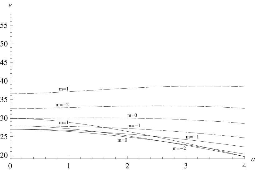
Figure 3: Dependence of $e$ on $a$ at $b=0.5$.

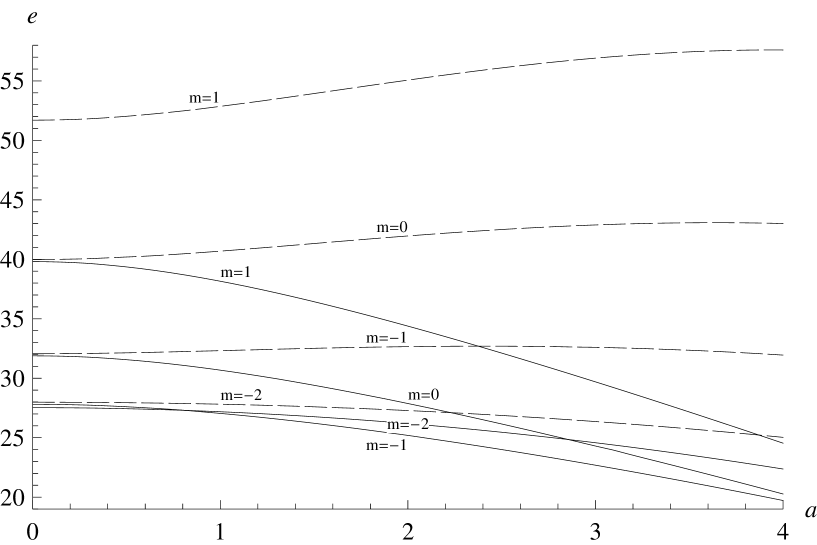
Figure 4: Dependence of $e$ on $a$ at $b=3$.

IV Conclusion

In our opinion, the examined exactly solvable model with the realistic potential well of finite depth is physically adequate in order to describe the behavior of an electron in a semiconductor quantum ring of finite width with account of the Rashba spin-orbit interaction in the presence of an external magnetic field.

Table 1: Dependence of $e$ on $r_{i}$ at $v=400,\,a=1,\,b=1$.

$r_{i}$	$m=-2$		$m=-1$		$m=0$		$m=1$
	$e$
0.1	11.1546	20.5634	8.40784	11.6889	8.07216	16.0687	14.7685	29.0068
0.3	15.2333	22.0607	14.8695	15.6909	14.4308	20.1349	18.7835	30.5326
0.5	26.6594	31.1076	27.0008	27.2145	26.6594	31.5576	30.1207	39.6641
0.7	60.0830	62.9589	60.2745	61.0963	60.4248	64.9463	63.4123	71.6304
0.9	217.766	219.587	217.804	219.066	218.264	222.606	220.965	228.388

Table 2: Dependence of $e$ on $v$ at $r_{i}=0.5,\,a=1,\,b=1$.

$v$	$m=-2$		$m=-1$		$m=0$		$m=1$
	$e$
25	11.1356	15.5883	11.0065	11.6889	10.4833	15.9651	14.5421	20.6312
50	15.0121	19.6818	15.2366	15.3623	14.7204	19.8905	18.4485	28.2691
100	19.1740	23.7577	19.4880	19.6275	19.0631	24.0567	22.6185	32.3247
400	26.6724	31.1076	27.0008	27.2145	26.6594	31.5576	30.1207	39.6634
1000	30.4209	34.8152	30.7516	30.9818	30.4279	35.3066	33.8699	43.3697

References

• (1) T.V. Bandos, A. Cantarero and A. Garcia-Cristóbal, Eur. Phys. J. B 53, 99-108 (2006).
• (2) M. Grochol, F. Grosse and R. Zimmermann, Phys. Rev. B 74, 115416 (2006).
• (3) A. V. Chaplik and L. I. Magarill, Phys. Rev. Lett. 96, 126402 (2006).
• (4) V.V. Kudryashov, Proc. of the XIII Intern. School-Conference ”Foundations and Advances in Nonlinear Science”, Minsk, 2006, pp. 125-130; Nonlinear Phenomena in Complex Systems 12, 199-203 (2009).
• (5) E.I. Rashba, Fiz. Tverd. Tela (Leningrad) 2, 1224 (1960) [Sov. Phys. Solid State 2, 1109 (1960)].
• (6) Yu.A. Bychkov and E.I. Rashba, J. Phys. C 17, 6039-6046 (1984).
• (7) V.V. Kudryashov, Proc. of the XIV Intern. School-Conference ”Foundations and Advances in Nonlinear Science”, Minsk, 2009, pp. 95-102.
• (8) E.N. Bulgakov and A.F. Sadreev, Pis’ma v ZhETF 73, 573 2001) [JETP Lett. 73, 505 (2001)].
• (9) E. Tsitsishvili, G.S. Lozano and A.O. Gogolin, Phys. Rev. B 70, 115316 (2004).
• (10) M. Abramovitz and I.A. Stegun (eds.), Handbook of Mathematical Functions ( Dover Publications, New York, 1970).