On the Periodicity of Oscillatory Reconnection

Abstract

Context. Oscillatory reconnection is a time-dependent magnetic reconnection mechanism that naturally produces periodic outputs from aperiodic drivers.

Aims. This paper aims to quantify and measure the periodic nature of oscillatory reconnection for the first time.

Methods. We solve the compressible, resistive, nonlinear MHD equations using 2.5D numerical simulations.

Results. We identify two distinct periodic regimes: the impulsive and stationary phases. In the impulsive phase, we find the greater the amplitude of the initial velocity driver, the longer the resultant current sheet and the earlier its formation. In the stationary phase, we find that the oscillations are exponentially decaying and for driving amplitudes $6.3-126.2\>$km/s, we measure stationary-phase periods in the range $56.3-78.9\>$s, i.e. these are high frequency ($0.01-0.02\>$Hz) oscillations. In both phases, we find that the greater the amplitude of the initial velocity driver, the shorter the resultant period, but note that different physical processes and periods are associated with both phases.

Conclusions. We conclude that the oscillatory reconnection mechanism behaves akin to a damped harmonic oscillator.

1 Introduction

Traditionally, magnetic reconnection and MHD wave theory have been viewed as separate areas of solar physics (see, e.g., Priest & Forbes magneticreconnection2000 (2000); Roberts Bernie (2004); De Moortel DeMoortel2005 (2005); Nakariakov & Verwichte NV2005 (2005); De Moortel & Nakariakov DN2012 (2012)). However, this is a misconception: we know that (steady-state) reconnection models not only generate outflows/waves, but also require inflows/waves (e.g. Parker Parker (1957); Sweet Sweet (1958); Petschek Petschek (1964)). Several authors have already challenged this point-of-view (e.g. Craig & McClymont CraigMcClymont1991 (1991); Longcope & Priest LP2007 (2007); Murray et al. Murray2009 (2009); McLaughlin et al. McLaughlin2009 (2009); McLaughlin2012 (2012)) and their investigations contribute to our understanding of dynamic or time-dependent models of magnetic reconnection. Of particular importance to this paper is the work of McLaughlin et al. (McLaughlin2009 (2009)) which is the first demonstration of reconnection naturally driven by MHD wave propagation, via a process entitled oscillatory reconnection.

MHD wave propagation in inhomogeneous media is a fundamental plasma process and the study of MHD waves in the neighbourhood of magnetic null points directly contributes to this area (see review by McLaughlin et al. McLaughlinREVIEW (2011)). It is known that null points - weaknesses in the magnetic field where the field strength, and hence the Alfvén speed, is zero - and separatrices - topological features that separate regions of different magnetic flux connectivity - are an inevitable consequence of the distributed isolated magnetic flux sources at the photospheric surface, where the number of such null points will depend upon the magnetic complexity of the photospheric flux distribution (see, e.g., review by Longcope L2005 (2005), and Close et al. Close2004 (2004); Régnier et al. RPH2008 (2008); Longcope & Parnell LP2009 (2009) for the statistics of coronal null points). It is also now known that MHD wave perturbations are omnipresent in the corona (e.g. Tomczyk et al. Tomczyk2007 (2007)). Thus, these two areas of scientific study; MHD waves and magnetic topology, will encounter each other in the corona, i.e. MHD waves will propagate into the neighbourhood of coronal null points (e.g. blast waves from a flare will at some point encounter a null point).

McLaughlin & Hood (MH2004 (2004); MH2005 (2005); 2006a ; 2006b ) investigated the behaviour of linear MHD waves (fast and slow magnetoacoustic waves and Alfvén waves) in the neighbourhood of a variety of 2D null points. It was found that the (linear) fast wave is focused towards the null point by a refraction effect and all the wave energy, and thus current density, accumulates close to the null, i.e. null points will be locations for preferential heating by (linear) fast waves. The Alfvén wave propagates along magnetic fieldlines and so accumulates along the separatrices (in 2D) or along the spine or fan-plane (in 3D). Waves in the neighbourhood of a single 2D null point have also been investigated using cylindrical models, in which the generated waves encircled the null point (e.g. Bulanov & Syrovatskii Bulanov1980 (1980); Craig & McClymont CraigMcClymont1991 (1991); CraigMcClymont1993 (1993); Craig & Watson CraigWatson1992 (1992); Hassam Hassam1992 (1992)) and it was found that the wave propagation leads to an exponentially-large increase in the current density (see also Ofman Ofman1992 (1992); Ofman et al. Ofman1993 (1993); Steinolfson et al. Steinolfson1995 (1995) and a comprehensive review by McLaughlin et al. McLaughlinREVIEW (2011) for further details). 3D MHD wave activity about coronal null points has been investigated by various authors (e.g. Galsgaard et al. Galsgaard2003 (2003); Pontin & Galsgaard P1 (2007); Pontin et al. P2 (2007); McLaughlin et al. MFH2008 (2008); Galsgaard & Pontin 2011a ; 2011b ; Thurgood & McLaughlin Thurgood2012 (2012)).

Reconnection can occur when strong currents cause the magnetic fieldlines to diffuse through the plasma and change their connectivity (Parker Parker (1957); Sweet Sweet (1958); Petschek Petschek (1964)). However, these papers did not include the effect of gas pressure, which would act to limit the growth of the current density. In considering the relaxation of a 2D X-type neutral point disturbed from equilibrium, Craig & McClymont (CraigMcClymont1991 (1991)) found that free magnetic energy is dissipated by a physical mechanism which couples resistive diffusion at the null to global advection of the outer field, which they called oscillatory reconnection. An example of oscillatory reconnection generated by magnetic flux emerging into a coronal hole was reported by Murray et al. (Murray2009 (2009)) who found a series of “reconnection reversals” take places as the system searches for equilibrium, i.e. the system demonstrates oscillatory reconnection in a self-consistent manner. The physics behind oscillatory reconnection has been investigated by McLaughlin et al. (McLaughlin2009 (2009)), Murray et al. (Murray2009 (2009)) and Threlfall et al. (Threlfall2012 (2012)).

McLaughlin et al. (McLaughlin2012 (2012)) investigated the long-term evolution of an initially-buoyant magnetic flux tube emerging into a gravitationally-stratified coronal hole environment and reported on the resulting oscillations and outflows. They found that the physical mechanism of oscillatory reconnection naturally generates quasi-periodic vertical outflows with a transverse/swaying aspect. There is currently a great deal of interest in observations of transverse motions in the solar atmosphere (e.g. Tomczyk et al. Tomczyk2007 (2007); De Pontieu et al. Bart2007 (2007); Bart2011 (2011); Cirtain et al. Cirtain2007 (2007); Erdélyi & Taroyan Robertus2008 (2008); Nishizuka et al. Nishizuka2008 (2008); Nishizuka2011 (2011); He et al. 2009a ; 2009b ; Liu et al. Liu2009 (2009); Liu2011 (2011); McIntosh et al. McIntosh2011 (2011); Okamoto & De Pontieu OBart2011 (2011); Morton et al. Morton2012 (2012); Yurchyshyn et al. Yurchyshyn2012 (2012)) and transverse/swaying motions have been observed over a range of wavelengths, speeds, temperatures and scales. However, the origin of these propagating, transverse oscillations remains a mystery, and these authors often note that the challenge remains to understand how and where these waves are generated in the solar atmosphere. Liu et al. (Liu2011 (2011)) summarises possible generation mechanisms for these transverse motions, including an oscillating wake from a coronal mass ejection or periodic reconnection (see, e.g., Chen & Priest CP2006 (2006); Sych et al. Sych2009 (2009)). The physical mechanism of oscillatory reconnection is another possible source of these transverse motions. As reported by McLaughlin et al. (McLaughlin2012 (2012)), the transverse behaviour seen in the periodic jets originating from the reconnection region of the inverted Y-shaped structure is specifically due to the oscillatory reconnection mechanism, and would be absent for a single, steady-state reconnection jet. The physical mechanism also naturally generates periodic outputs even though no periodic driver is imposed on the system.

Thus, there is a clear interest in furthering our understanding of the periodic nature of oscillatory reconnection. In this paper, we investigate the periodic signal generated by the mechanism, with a specific interest in measuring periods and decay rates as well as the robustness of our results, i.e. how do the results vary with the strength of the driver.

1.1 Overview of McLaughlin et al. (2009)

This paper will closely follow the work of McLaughlin et al. (McLaughlin2009 (2009)) as we investigate the periodic nature of oscillatory reconnection. These authors investigated the behaviour of nonlinear fast magnetoacoustic waves near a 2D X-type neutral point and found that the incoming wave deforms the null point into a cusp-like point which in turn collapses to a current sheet. The system then evolves periodically through a series of horizontal/vertical current sheets with associated changes in connectivity, i.e. the system demonstrates the mechanism of oscillatory reconnection.

More specifically, McLaughlin et al. (McLaughlin2009 (2009)) found that the incoming (fast) wave propagates across the magnetic fieldlines and the initial profile, an annulus, contracts as the wave approaches the null point. This is the refraction behaviour that is typical of fast wave behaviour around magnetic null points (see, e.g., McLaughlin et al. McLaughlinREVIEW (2011)) and results from the spatially-varying (equilibrium) Alfvén-speed profile.

The incoming wave was observed to develop discontinuities (for a physical explanation, see Appendix B of McLaughlin et al. McLaughlin2009 (2009) or, alternatively, Gruszecki et al. Marcin2011 (2011)) and these discontinuities form fast oblique magnetic shock waves, where the shock makes ${\bf{B}}$ refract away from the normal. Interestingly, the shock locally heats the initially $\beta=0$ plasma, creating $\beta\neq 0$ at these locations.

At a later time, the shocks overlap, forming a shock-cusp, which leads to the development of hot jets and in turn these jets substantially heat the local plasma and significantly deform the local magnetic field. By the time the shock waves reach the null, the (initially X-point) magnetic field has been deformed such that the separatrices now touch one another rather than intersecting at a non-zero angle (Priest & Cowley PC1975 (1975) call this ‘cusp-like’). The osculating field structure continues to collapse and forms a horizontal current sheet. However, the separatrices continue to evolve: the jets at the ends of the (horizontal) current sheet continue to heat the local plasma, which in turn expands. This expansion squashes and shortens the current sheet, forcing the separatrices apart. The (squashed) current sheet thus returns to a ‘cusp-like’ null point that, due to the continuing expansion of the heated plasma, in turn forms a vertical current sheet. In effect, the (net) restoring force acts to return the (deformed) null point to its equilibrium state, but overshoots the equilibrium. The phenomenon then repeats itself: jets heat the plasma at the ends of this newly-formed (vertical) current sheet, the local plasma expands, the (vertical) current sheet is shortened, the system attempts to return itself to equilibrium, overshoots and forms a (second) horizontal current sheet. The evolution proceeds through a series of horizontal and vertical current sheets, and the system clearly displays oscillatory behaviour. It is also interesting to note that the final state is non-potential, where this is because the plasma to the left and right of the null is (locally) hotter than that above and below. Consequently, a thermal-pressure gradient exists and causes the X-point to be slightly closed up in the vertical direction (i.e. generating a small, positive current). It is important to note that the non-potential final state is still in force balance and will eventually return to a potential state, but on a far greater timescale than our simulations ($t_{{\rm{diffusion}}}\sim R_{m}=10^{4}$ Alfvén times, where $R_{m}$ is the magnetic Reynolds number). We also note that there is nothing unique about the orientation of the first current sheet being horizontal followed by a vertical, this simply results from the particular choice of initial condition, and McLaughlin et al. (McLaughlin2012 (2012)) use the more general terminology orientation 1 and orientation 2.

McLaughlin et al. (McLaughlin2009 (2009)) also present evidence of reconnection occurring in the system; reporting both a change in fieldline connectivity (qualitative evidence) and changes in the vector potential which directly showed a cyclic increase and decrease in magnetic flux on either side of the separatrices (see their Figures 12 and 13). Hence, since the system displayed both oscillatory behaviour and reconnection, it was concluded that the system demonstrated the phenomenon of oscillatory reconnection.

Our paper has the following outline: the basic setup, equations and assumptions are described in §2, the periodic nature of oscillatory reconnection is detailed in §3 and the conclusions are given in §4.

2 Basic Equations

We consider the nonlinear, compressible, resistive MHD equations:

$$\rho\left[{\partial{\bf{v}}\over\partial t}+\left({\bf{v}}\cdot\nabla\right){\bf{v}}\right] = -\nabla p+\left({{\frac{1}{\mu}}}\nabla\times{\bf{B}}\right)\times{\bf{B}}\;,$$

$${\partial{\bf{B}}\over\partial t} = \nabla\times\left({\bf{v}}\times{\bf{B}}\right)+\eta\nabla^{2}{\bf{B}}\;,$$

$$\rho\left[{\partial{\epsilon}\over\partial t}+\left({\bf{v}}\cdot\nabla\right){\epsilon}\right] = -p\nabla\cdot{\bf{v}}+{{\frac{1}{\sigma}}}\left|{\bf{j}}\right|^{2}+Q_{\rm{shock}}\;,$$

$${\partial\rho\over\partial t}+\nabla\cdot\left(\rho{\bf{v}}\right) = 0\;,$$ (1)

where $\rho$ is the mass density, ${\bf{v}}$ is the plasma velocity, ${\bf{B}}$ the magnetic induction (usually called the magnetic field), $p$ is the plasma pressure, $\mu=4\pi\times 10^{-7}\/\mathrm{Hm^{-1}}$ is the magnetic permeability, $\sigma$ is the electrical conductivity, $\eta=1/{\mu\sigma}$ is the magnetic diffusivity, $\epsilon={p/\rho\left(\gamma-1\right)}$ is the specific internal energy density, $\gamma={5/3}$ is the ratio of specific heats and ${\bf{j}}={{\nabla\times{\bf{B}}}/\mu}$ is the electric current density.

We solve these governing equations numerically using a Lagrangian remap, shock-capturing code called LARE2D (Arber et al. Arber2001 (2001)), which utilizes artificial shock viscosity to introduce dissipation at steep gradients. The details of this technique, often called Wilkins viscosity, can be found in Wilkins (Wilkins1980 (1980)). Thus, $Q_{\rm{shock}}$ represents the viscous heating at shocks.

We now introduce a change of scale to non-dimensionalise all variables. Letting ${\rm{\bf{v}}}={\rm{v}}_{0}{\mathbf{v}}^{*}$, ${\mathbf{B}}=B{\mathbf{B}}^{*}$, $x=Lx^{*}$, $y=Ly^{*}$, $z=Lz^{*}$, $\rho={\rho}_{0}\rho^{*}$, $p=p_{0}p^{*}$, ${\bf{j}}=j_{0}\>{\bf{j}}^{*}$, $\nabla=\nabla^{*}/L$, $t={t}_{0}t^{*}$ and $\eta=\eta_{0}$, where * denotes a dimensionless quantity and ${\rm{v}}_{0}$, $B$, $L$, ${\rho}_{0}$, $p_{0}$, $j_{0}$, ${t}_{0}$ and $\eta_{0}$ are constants with the dimensions of the variable they are scaling. We then set ${B}/{\sqrt{\mu\rho_{0}}}={\rm{v}}_{0}$ and ${\rm{v}}_{0}={L}/{{t_{0}}}$ (this sets ${\rm{v}}_{0}$ as a constant background Alfvén speed). We also set $j_{0}=B/\mu L$ and ${\eta_{0}{t}_{0}}/{L^{2}}=R_{m}^{-1}$, where $R_{m}$ is the magnetic Reynolds number, and choose $R_{m}=10^{4}$. This process non-dimensionalises equations (1) and under these scalings, $t^{*}=1$ (for example) refers to $t={t}_{0}={L}/{{\rm{v}}_{0}}$; i.e. the time taken to travel a distance $L$ at the background Alfvén speed.

There is no fixed dimensional length scale to our X-point system (X-points are scale-free), and thus we have a great deal of freedom in choosing our dimensional constants. We choose $L=1\>$Mm and $B=1\>$G (for simplicity, and where these choices allow an intuitive understanding of equation 2 below) and we chose a coronal density of ${\rho}_{0}=5\times 10^{-13}\>$kg/m³ and coronal temperature of $T_{0}=10^{6}\>$K. This sets ${\rm{v}}_{0}={B}/\sqrt{\mu\rho_{0}}=126.2\>$km/s, $t_{0}={L}/{{\rm{v}}_{0}}=7.93\>$seconds and $j_{0}=B/\mu L=8\times 10^{-5}\>$A. The values returned from equations (1) are made dimensional using these solar constants.

2.1 Basic equilibrium and numerical set-up

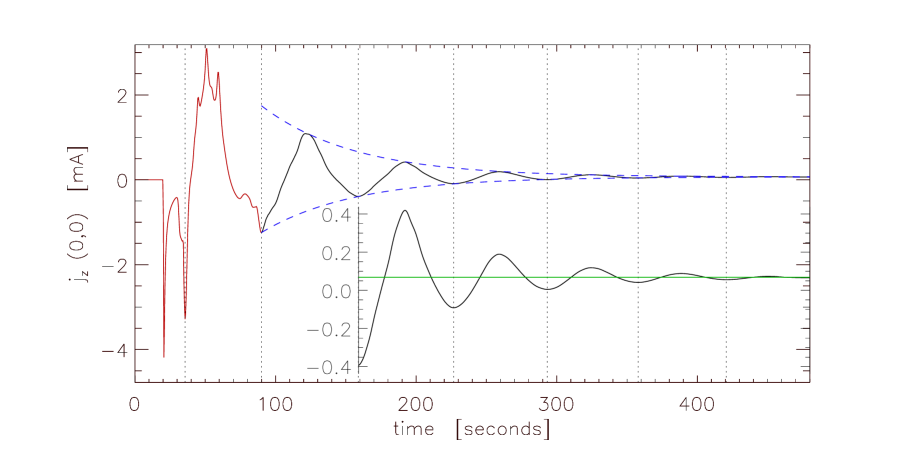
Figure 1: Plot of time evolution of $j_{z}(0,0,t)$ (measured in milliAmps) for $0\leq t\leq 480\>$seconds. Red line indicates impulsive phase and black line indicates stationary phase. Insert shows the same time evolution over $158.9\leq t\leq 480\>$seconds (same horizontal axis, different vertical axis). The black dotted lines indicate the formation times of all the horizontal current sheets and the green line indicates $j_{{\rm{final}}}=0.8165j_{0}=6.5\times 10^{-5}\>$A. The blue dashed lines indicate an exponentially-damped envelope ${\rm{max}}(j_{z})|_{\rm{stationary}}\times e^{-\lambda t}+j_{{\rm{final}}}$ and ${\rm{min}}(j_{z})|_{\rm{stationary}}\times e^{-\lambda t}+j_{{\rm{final}}}$ where $\lambda=-0.015\>{\rm{s}}^{-1}$.

To set-up our system, we follow the numerical framework of McLaughlin et al. (McLaughlin2009 (2009)). Thus, we consider a simple 2D X-type neutral point as our equilibrium magnetic field, where the initial field is taken as:

$${\bf{B}}_{0}=\frac{B}{L}\left(y,x,0\right)\;,$$ (2)

where $B=1\>$G is a characteristic field strength and $L=1\>$Mm is the length scale for magnetic field variations. This magnetic field can be seen in McLaughlin et al. (McLaughlin2009 (2009), their Figure 1).

Initially, we consider the equilibrium plasma to be cold: $T=0\>$K (i.e. $\beta(t=0)=0$) and, hence, ignore plasma pressure effects. However, McLaughlin et al. (McLaughlin2009 (2009)) showed that magnetic shocks will heat the plasma and so the plasma will not remain cold (see e.g. $\S 1.5$ in Priest & Forbes magneticreconnection2000 (2000)).

In order to excite a pure fast magnetoacoustic wave, we consider an initial condition that perturbs velocity purely across the equilibrium magnetic field. Using the terminology of McLaughlin et al. (McLaughlin2009 (2009)), there are three distinguishing velocity components that can be considered in our system:

• ${\rm{v}}_{\perp}={\bf{v}}\times{\bf{B}}_{0}\cdot{\hat{\bf{z}}}={\rm{v}}_{x}B_{y}-{\rm{v}}_{y}B_{x}$, which corresponds to the velocity across the equilibrium field, and hence corresponds to the fast magnetoacoustic wave (the only MHD wave that can cross fieldlines),

• ${\rm{v}}_{\parallel}={\bf{v}}\cdot{\bf{B}}_{0}={\rm{v}}_{x}B_{x}+{\rm{v}}_{y}B_{y}$, which corresponds to the velocity along the equilibrium field and corresponds to the propagation of the slow magnetoacoustic wave,

• ${\rm{v}}_{z}={\bf{v}}\cdot{\hat{\bf{z}}}$, which corresponds to the velocity in the invariant direction and hence corresponds to the Alfvén wave.

Interestingly, these three velocity components - each isolating an individual MHD mode - are in good agreement with those reported by Thurgood & McLaughlin (Thurgood2012 (2012)) who used the equilibrium magnetic field and the flux function (which is parallel to the invariant direction) to define an orthogonal coordinate system to isolate and identify the propagation of each of the MHD modes. Using their convention, ${\rm{v}}_{\perp}={\bf{v}}\cdot{{\bf{B}}}_{0}\times{\hat{{\bf{A}}}}$, where ${\bf{A}}=\frac{1}{2}\left(y^{2}-x^{2}\right){\hat{\bf{z}}}$ is the flux function, and where perturbations in the ${\bf{B}}_{0}\times\hat{{\bf{A}}}$-direction were shown to correspond to those of the fast wave (for helicity-free systems, such as our 2D X-point).

To perturb our system, we consider an initial condition in velocity such that:

$${\rm{v}}_{\perp}\left(x,y,t=0\right) = 2C\sin\left[\pi\left(r-4.5\right)\right]{\rm{\;\;for\;\;\;}}4.5\leq r\leq 5.5\;,$$

$${\rm{v}}_{\parallel}\left(x,y,t=0\right) = {\rm{v}}_{z}\left(x,y,t=0\right)=0\;$$ (3)

where $r^{2}=x^{2}+y^{2}$ and $2C$ is our initial amplitude and initial condition (3) describes a circular, sinusoidal pulse in ${\rm{v}}_{\perp}$. Thus, as argued above, we initially generate (only) a pure fast wave in our system. Note that the velocity profile prescribed by equation (3) appears as the symmetric $m=0$ mode in ${{\rm{v}}_{\perp}}$, but corresponds to the asymmetric $m=2$ mode in Cartesian components. This is why the first current sheet has horizontal orientation, as per §1.1.

This initial pulse will naturally split into two waves - an outgoing wave and an incoming wave - each of amplitude $C$. In this paper, we will focus on the incoming wave, i.e. the wave propagating towards the null point. In this paper, we will conduct a parameter study of initial wave amplitude $C$. Note that setting $C=1$ recovers the results of McLaughlin et al. (McLaughlin2009 (2009)) and choosing a small value for $C$, say $C=0.001$, recovers the the linear results from McLaughlin & Hood (MH2004 (2004); i.e. see Appendix A of McLaughlin et al. McLaughlin2009 (2009)). Under our dimensionalisation, a choice of $C=1$ corresponds to an incoming wave with maximum initial Cartesian velocity ${{\rm{v}}_{\perp}}/r={\rm{v}}_{0}/5=25.2\>$km/s at a distance of $r=5L=5\>$Mm and an equilibrium magnetic field strength of $5\>$G.

The governing equations (1) with initial conditions (3) are solved computationally in a square domain $x,y\in[-20,20]$ with a numerical resolution of $6144\times 6144$. Zero gradient boundary conditions are applied to the variables ${\bf{B}}$, $\rho$, $\epsilon$ at the four boundaries, and ${\bf{v}}$ is set to zero on all boundaries, i.e. reflective boundaries. A numerical damping region exists for $x^{2}+y^{2}\geq 6$ which gradually removes kinetic energy from the outgoing waves and so all oscillations that enter this region are slowly damped away, and hence they do not influence the behaviour about the null. The (equilibrium) Alfvén speed increases with distance from the null point and, hence, waves accelerate as they propagate outwards. Since we do not want reflected waves to influence our null point, implementation of such a damping region is essential.

3 Aperiodic driver leading to periodic behaviour

We set $C=1$ in equations (3) and, as expected, we recover the results of McLaughlin et al. (McLaughlin2009 (2009)) and readers are directed to that paper for full details (primarily their Figures 2, 5 & 6) and also this paper’s $\S\ref{section1.1}$. One of the key results from McLaughlin et al. (McLaughlin2009 (2009)) was the production of a periodic response resulting from an aperiodic input, i.e. the physical mechanism of oscillatory reconnection naturally gave rise to periodic behaviour. This periodic response can be quantitatively measured by analysing the time evolution of the (electric) current density, specifically ${\bf{j}}=(0,0,j_{z})$, at the null point itself. This can be seen in McLaughlin et al. (McLaughlin2009 (2009), their Figure 10) and the analysis of this time signal is the primary focus of this paper. In recreating the simulations of McLaughlin et al. (McLaughlin2009 (2009)), we recover this periodic time series, but at a higher numerical resolution, $6144\times 6144$, and at a higher cadence, $dt=0.05\>t_{0}$. The time evolution of $j_{z}(0,0,t)$ for $0\leq t\leq 480\>$s can be seen in Figure 1. Note that due to the symmetry of our system, the null is always located at the origin.

We identify two distinct regimes in Figure 1: $0\leq t<90\>$s (red line in Figure 1) which we refer to as the impulsive phase and $t\geq 90\>$s (black line in Figure 1) which we refer to as the stationary phase. The impulsive (or transient) phase is a spiky, irregular signal, with multiple local extrema indicating: the arrival time of the shock-cusp at the null point (at $t=20.6\>$s), the formation of the first horizontal current sheet (at $t=35.7\>$s, $j_{z}<0$), the formation of the first vertical current sheet (at $t=59.1\>$s, $j_{z}>0$) and the formation of the second horizontal current sheet (at $t=90.0\>$s). The (current-sheet) signal is further contaminated due to addition of small currents related to the propagation of shock waves across the null point. We define the end of the impulsive phase as the formation time of the second horizontal current sheet, which in our $C=1$ simulation occurs at $t=90.0\>$s.

After $t=90.0\>$s, the evolution of $j_{z}(0,0,t)$ is much cleaner and closer to (damped) sinusoidal. For $t\geq 90.0\>$s, the extrema exactly match the formation of the cyclic current sheets, with $j_{z}<0\>$/$\>>0$ indicating horizontal/vertical current sheets, respectively. We define this ‘cleaner signal’ regime as the stationary phase, i.e. the regime characterised by a (damped) sinusoidal signal after the transients of the impulsive phase have leaked away, and this phase starts at the formation time of the second horizontal current sheet. The black dotted lines in Figure 1 indicate the formation times of all the horizontal current sheets (for both phases).

Note that in labelling these two regimes, i.e the impulsive phase and the stationary phase, we have adopted the terminology usually associated with the excitation and damping of trapped and leaky modes in coronal loop oscillations (see, e.g., Terradas et al. Terradas2005 (2005); Terradas2006 (2006); Luna et al. Luna2008 (2008); McLaughlin & Ofman MO2008 (2008) and reference therein).

Figure 2: Plot of $(a)$ formation time (measured in seconds) and $(b)$ length (measured in km and evaluated at the formation time) of first horizontal current sheet versus initial velocity amplitude (measured in km/s), where ${\rm{v}}_{0}=25.2\>$km/s corresponds to $C=1$ simulation.

3.1 Impulsive Phase

Let us consider the impulsive phase of the evolution of $j_{z}(0,0,t)$, i.e. evolution over $0\leq t<90$ (indicated by red line in Figure 1). We see that $j_{z}(0,0,t)$ is zero (since the equilibrium is potential) until the arrival of the fast oblique magnetic shock (which has its own associated current density) at the null point, indicated by the first (negative) extrema at $t=20.6\>$s. This is followed by a second (local) minimum at $t=35.7\>$s, which is the formation time of the first horizontal current sheet (i.e. not at $t=20.6\>$s). The correspondence between extrema and current-sheet formation cannot be deduced from Figure 1 alone, but can be determined by comparison with the evolution of the separatrices and contours of ${\bf{v}}$. The value of $j_{z}(0,0,t=35.7)=-41.25j_{0}=-3.3\>$mA is proportional to the length of the first horizontal current sheet, which is measured directly from the numerical simulation as $0.1162\>L=116.2\>$km (for the $C=1$ simulation).

The formation time and length (at formation time) of the first horizontal current sheet is of key interest here, since this directly reflects the driver (akin to a forcing term) of the system. We investigate how the formation time and length of the first horizontal current sheet vary as functions of the initial driving amplitude (from equation 3). Figure 2a shows the formation time (measured in seconds) of the first horizontal current sheet as a function of initial velocity amplitude (measured in km/s), where ${\rm{v}}_{0}=25.2\>$ corresponds to $C=1$ simulation. We see that the greater the driving amplitude, the earlier the first current sheet forms. This is intuitive as we expect fast oblique magnetic shocks with a larger amplitude to propagate faster and thus reach the null point more rapidly, compared to waves driven with a smaller amplitude.

Figure 2b shows how the current sheet length (measured in km) evaluated at the formation time of the first horizontal current sheet varies as a function of initial velocity amplitude. We see that the greater the driving amplitude, the longer the horizontal current sheet. The length of the current sheet is also directly proportional to the value of $j_{z}(0,0)$, and so we also conclude that the greater the driving amplitude, the stronger the value of $|j_{z}(0,0)|$ at the corresponding time. Again, this result is intuitive; it is the fast oblique magnetic shock that physically deforms the X-point into an osculating field structure (and ultimately into a horizontal current sheet) and thus we would expect stronger fast oblique magnetic shocks (i.e. with a larger amplitude) to deform, i.e. refract ${\bf{B}}$ away from the normal, and ‘squash’ the magnetic field to a greater extent, and thus to form longer and stronger current sheets.

Figure 3: Plot of impulsive period, i.e. time taken to evolve from the first horizontal current sheet to the second horizontal current sheet (measured in seconds) versus initial velocity amplitude (measured in km/s), where ${\rm{v}}_{0}=25.2\>$km/s corresponds to $C=1$ simulation.

Figure 4: Plot of $(a)$ stationary period, i.e. the time taken to evolve from the second horizontal current sheet to the third (measured in seconds) and $(b)$ $j_{{\rm{final}}}$, i.e. $j_{z}(0,0)$ evaluated at $t=480\>$s, (measured in milliAmps) versus initial velocity amplitude (measured in km/s), where ${\rm{v}}_{0}=25.2\>$km/s corresponds to $C=1$ simulation.

Finally, let us investigate the time taken to evolve from the first horizontal current sheet (at $t=35.7\>$s) to the formation time of the second horizontal current sheet (at $t=90.0\>$s for the $C=1$ simulation), namely the time taken for one complete cycle (i.e. horizontal current sheet evolves to vertical, evolves back to horizontal). This time, which we refer to as the impulsive period, is calculated to be $t=54.3\>$s (for initial amplitude ${\rm{v}}_{0}=25.2\>$km/s in the $C=1$ system). Again, we now investigate how this impulsive period varies with the initial driving amplitude ($\propto C{\rm{v}}_{0}$) and this can be seen in Figure 3. Here, we see that the greater the initial driving amplitude, the shorter the resulting impulsive period, i.e. the shorter the time taken to evolve from the first horizontal current sheet to the second. Recalling the dependency seen Figure 2b, this means that for longer current sheets, the impulsive period is shorter. This means that the restoring force must be stronger and so we conclude that longer current sheets have a stronger restoring force. In this way, the system acts as a harmonic oscillator, i.e. the greater the displacement away from equilibrium, the stronger the restoring force.

3.2 Stationary Phase

Let us now investigate the stationary phase of the oscillation seen in Figure 1 (black line), i.e. the time evolution of $j_{z}(0,0,t)$ for $t_{2}\leq t\leq 480\>$s, where $t_{2}$ is the formation time of the second horizontal current sheet ($t_{2}=90.0\>$s for the $C=1$ simulation). Figure 1 also has an insert showing the (same) time evolution of $j_{z}(0,0,t)$ for $158.9\leq t\leq 480\>$s, i.e. same horizontal time axis, different vertical axis. Note that the insert does not show the start of the stationary phase, only a later part of it (starting at the time of the third horizontal current sheet). The green line indicates $j_{{\rm{final}}}$, i.e. the finite amount of current density left in the system at $t=480\>$s when the system has reached its final, non-potential state. For the $C=1$ system, this final state occurs at $t=480\>$s (8 mins) and $j_{{\rm{final}}}=0.8165j_{0}=6.5\times 10^{-5}\>$A.

We see that there is clear oscillatory behaviour in the stationary phase and, moreover, the oscillation is exponentially decaying. This can be seen in Figure 1 and the blue dashed lines indicate an exponentially-damped envelope ${\rm{max}}(j_{z})|_{\rm{stationary}}\times e^{-\lambda t}+j_{{\rm{final}}}$ and ${\rm{min}}(j_{z})|_{\rm{stationary}}\times e^{-\lambda t}+j_{{\rm{final}}}$ where $\lambda=-0.015\>{\rm{s}}^{-1}$ is determined experimentally.

Let us now investigate the period associated with the stationary phase, which we define as the time taken to evolve between horizontal current sheets. Specifically, we define the stationary period as the time taken to evolve from the second horizontal current sheet to the third, i.e. the first complete oscillation within the stationary phase. For the $C=1$ simulation, these formation times are $90.0\>$s and $158.9\>$s resulting in a stationary period of $69.0\>$s (note we present results here correct to 1 decimal places, but calculate periods to a greater degree of accuracy). Similar results are obtained for alternative definitions of the stationary periods, e.g. time taken to evolve from one vertical current sheet to the next.

We now investigate how the stationary period varies with the initial driving amplitude and this can be seen in Figure 4a. Here, we see that the greater the initial driving amplitude, the shorter the resulting stationary period. Thus, these results are in agreement with those in $\S\ref{section4.1}$, i.e. the stronger the initial driving amplitude, the longer the resulting current sheet, thus the stronger the restoring force, thus the shorter the resulting period. Coupled with the exponential decay, we see that in the stationary phase, the system acts akin to a damped harmonic oscillator.

We also measure all the proceeding oscillations in the stationary phase, i.e. time taken to evolve from the second/third horizontal current sheet to the third/fourth horizontal current sheet, and obtain similar periods of $67.8\>$s and $66.6\>$s respectively. Interestingly, this means that the stationary period appears to be slightly decreasing by roughly $1.8\%$ per oscillation.

Finally, we investigate $j_{{\rm{final}}}$, the finite amount of current density left in the system when the system has reached its final, non-potential state and this can be seen in Figure 4b. For the $C=1$ system, $j_{{\rm{final}}}=0.8165j_{0}=6.5\times 10^{-5}\>$A which is measured at $t=480\>$s. In all our simulations, $j_{{\rm{final}}}>0$ indicating that the (final) X-point is very slightly closed up in the vertical direction, i.e. $j_{z}>0$ is associated with vertical current sheets. This is because the (local) plasma to the left and right of the X-point is slightly hotter, since that is where the initial, strongest jet heating occurs. Thus, the existence of this thermal-pressure gradient coupled with force balance requires the final state to be non-potential.

From Figure 4b, we see that the stronger the initial driving amplitude, the greater the value of $j_{{\rm{final}}}$. Again, this is intuitive: fast oblique magnetic shocks with a larger amplitude will intersect to form stronger, hotter jets to the left and right of the X-point. Thus, this local plasma will be hotter at the end of the simulation, indicating a stronger thermal-pressure gradient and thus, in order to achieve force balance, a greater absolutely value of the Lorentz force, i.e. a greater value of $j_{{\rm{final}}}$.

4 Conclusions

This paper describes an investigation into the periodicity of oscillatory reconnection, specifically oscillatory reconnection initiated by a nonlinear fast magnetoacoustic wave deforming a 2D magnetic X-point. We have solved the compressible, resistive, nonlinear MHD equations using a Lagrangian remap, shock-capturing code (LARE2D) and have followed the numerical set-up of McLaughlin et al. (McLaughlin2009 (2009)). As in that paper, we find that the fast magnetoacoustic wave develops into a fast oblique magnetic shock wave which significantly deforms the local magnetic fieldlines, to the extent that the incoming wave deforms the null point into a cusp-like point which in turn collapses to a current sheet. The system then evolves periodically through a series of horizontal and vertical current sheets with associated changes in connectivity, i.e. the system demonstrates the mechanism of oscillatory reconnection.

The main focus of this paper is on the periodic nature of this oscillatory cycle of horizontal and vertical current sheets. For the first time, we identify two distinct phases in the oscillation: a transient, impulsive phase, encompassing the development of the first horizontal current sheet, the formation of the first vertical current sheet, and ending with the formation of the second horizontal current sheet. We define the stationary phase to begin at the formation of the second horizontal current sheet and thus this phase includes all the proceeding cyclic behaviour.

In the impulsive phase, we find that greater the driving amplitude ($C{\rm{v}}_{0}$) of the velocity initial condition (equation 3), [a] the earlier the first horizontal current forms, [b] the longer its maximum length and [c] the greater its maximum current density. These results are intuitive since we would expect magnetic shocks with larger amplitudes to propagate faster and thus arrive at the null point more rapidly than those with smaller amplitudes. We would also expect magnetic shocks with larger amplitudes to deform the pre-existing magnetic field to a greater extent (specifically to refract ${\bf{B}}$ away from the normal to a greater extent) and thus, ultimately, to form longer and stronger current sheets.

We also investigate the time taken to evolve from the first horizontal current sheet to the second, which we labelled as the impulsive period. We find that the greater the initial velocity amplitude ($C{\rm{v}}_{0}$) the shorter the resultant impulsive period. Coupled with the results on current sheet length, this means that longer current sheets have shorter corresponding impulsive periods. In this way, the system is acts as a harmonic oscillator, i.e. the greater the displacement away from equilibrium, the stronger the restoring force, and thus the shorter the impulsive period.

For a driving amplitude of $25.2\>$km/s (corresponding to $C=1$ simulation) we measure an impulsive period of $54.3\>$s. We also investigate the resultant impulsive periods for driving amplitudes $6.3-126.2\>$km/s and find associated impulsive periods in the range $46.9-65.4\>$s.

The stationary phase is found to be dominated by an exponentially-decaying oscillation, tending to a finite value, $j_{{\rm{final}}}$. We also investigate the stationary period, namely the time taken to evolve from the second horizontal current sheet to the third, i.e. the first complete cycle of the stationary phase. As in the impulsive phase, we find that the greater the initial velocity amplitude ($C{\rm{v}}_{0}$) the shorter the resultant stationary period. This is explained just as before, the greater the initial amplitude, the longer and stronger the current sheets at each stage, and thus the greater restoring force, leading to shorter periods (compared to smaller initial amplitude, shorter resultant current sheets, weaker restoring force and thus longer periods). Hence, again the system acts as a harmonic oscillator and, coupled with the exponential decay, we relate the oscillatory reconnection mechanism to that of a damped harmonic oscillator during the stationary phase.

For a driving amplitude of $25.2\>$km/s (corresponding to $C=1$ simulation) we measure a stationary period of $69.0\>$s. We also investigate the resultant stationary periods for driving amplitudes $6.3-126.2\>$km/s and find associated stationary periods in the range $56.3-78.9\>$s, i.e. these are high frequency ($0.0127-0.0178\>$Hz) oscillations.

It is also prudent at this stage to ask what determines this stationary period and what determines the exponentially-decaying timescale. To this end, we can consider the work of Craig & McClymont (CraigMcClymont1991 (1991)) who investigated the relaxation of a 2D X-point disturbed from equilibrium. By neglecting both nonlinear and thermal pressure effects, Craig & McClymont (CraigMcClymont1991 (1991)) derived an analytical prediction for two timescales:

$$\qquad t_{\rm{oscillation}}\approx 2\ln{R_{m}}\;,\quad t_{\rm{decay}}\approx t_{\rm{oscillation}}^{2}/2\pi^{2}\;$$

where we identify $t_{\rm{oscillation}}$ as our stationary period and $t_{\rm{decay}}$ as our decay time; $1/\lambda$. For a driving amplitude of $25.2\>$km/s, these correspond to $t_{\rm{oscillation}}\approx 109.6\>$s, compared to our measured stationary period of $69.0\>$s, and $t_{\rm{decay}}\approx 76.7\>$s compared to our measured decay time of $1/\lambda=1/0.015=66.7\>$s, given that in our investigations $R_{m}=10^{4}$ and time is made dimensional using $t_{0}=7.93\>$s. Thus, given the (relative) simplicity of the Craig & McClymont (CraigMcClymont1991 (1991)) system, these estimates are in fair agreement with our results. Note, however, that these simple analytical formulae cannot predict the variation in period versus amplitude of the initial velocity driver. This suggests that nonlinear effects and thermal-pressure gradients play a crucial role, which seems reasonable given that the restoring force of oscillatory reconnection has been shown to be a dynamic competition between the thermal-pressure gradients and the Lorentz force (see $\S 3.2$ of Murray et al. Murray2009 (2009); $\S 3.3$ of McLaughlin et al. McLaughlin2009 (2009); Figure 7 of Threlfall et al. Threlfall2012 (2012)).

It is also important to note that there is a significant difference between the impulsive period (e.g. $54.3\>$s for $C=1$ system) and the stationary period (e.g. $69.0\>$s for the $C=1$ system), and that in every numerical experiment we find that the stationary period is longer than the impulsive period. This indicates that different physical processes dominate in each phase (i.e. the deformation of the X-point by the shock and the importance of jet heating in the impulsive phase, and the elastic motion of the magnetic field trying to get back to equilibrium in the stationary phase) and validates our approach of dividing the whole evolution into two distinct phases.

This difference in impulsive and stationary periodicities actually has an intriguing caveat : it is important to note that when oscillatory reconnection is seen in, say, a numerical simulation, one must be careful to interpret which phase one is actually observing and to observe several oscillations, i.e. if only two periods are seen, say the impulsive period followed by a single stationary period, then one would conclude that the period was actually increasing between oscillations. A similar result would pertain in solar observations of oscillatory reconnection, i.e. the first period measured would be shorter than the proceding periods (assuming the first, i.e. impulsive, period is also observed). This is a clear prediction for the oscillatory reconnection mechanism.

It is also important to note that, as shown by McLaughlin et al. (McLaughlin2012 (2012)), the mechanism periodically generates ${\rm{v}}_{x}$ and ${\rm{v}}_{y}$ but that these are generated exponentially damped. Thus, if such signals are detected, then they may be decaying not due to a particular damping mechanism, but due to the generation mechanism itself.

In addition to the stationary period, we also measured all the proceeding periods in the stationary phase, e.g. time taken to evolve from third horizontal current sheet to fourth, etc. Interestingly, it was found that the period very slightly decreases by roughly $1.8\%$ per oscillation. The exact reason for this decrease in the period is uncertain and may be a numerical effect. This will be investigated further in future work.

As in McLaughlin et al. (McLaughlin2009 (2009)), it was found that the final state (i.e. velocity zero, oscillatory behaviour ceased) is in force balance but is non-potential and a small, finite amount of current density exists in the system, $j_{{\rm{final}}}$. The (final) X-point is very slightly closed up in the vertical direction, i.e. $j_{z}>0$ is associated with vertical current sheets. This is because the (local) plasma to the left and right of the X-point is slightly hotter, since that is where the initial, strongest, jet heating occurs. Thus, the existence of this thermal-pressure gradient in force balance requires the final state to be non-potential. We find that the greater the initial velocity amplitude ($C{\rm{v}}_{0}$) the larger the value of $j_{{\rm{final}}}$. Again, this is intuitive: fast oblique magnetic shocks with a greater amplitude will overlap to form stronger, hotter jets to the left and right of the (equilibrium) X-point. Thus, this local plasma will be hotter at the end of the simulation, indicating a stronger thermal-pressure gradient and thus, in order to achieve force balance, a greater value of the Lorentz force, i.e. a larger value of $j_{{\rm{final}}}$.

We have presented an investigation into the periodic nature of oscillatory reconnection and have found that an aperiodic driver can naturally generate a period signal via the physical mechanism of oscillatory reconnection. We have found that the system behaves akin to a damped harmonic oscillator. Again, this is not surprising: effectively our velocity initial condition can be thought of as injecting a finite amount of energy into the oscillatory reconnection mechanism and so intuitively the resultant periodic behaviour must be finite in duration, i.e. this is a dynamic reconnection phenomena as opposed to the classical steady-state, time-independent reconnection models.

Oscillatory Reconnection may also play a role in generating quasi-periodic pulsations (see, e.g., reviews by Aschwanden Aschwanden2003 (2003); Nakariakov & Melnikov Nakariakov2009 (2009)). Oscillatory behavior has been reported in a number of solar and stellar flare observations (e.g. Mathioudakis et al. Mathioudakis2003 (2003); Mathioudakis2006 (2006); McAteer et al. McAteer2005 (2005); Inglis et al. Inglis2008 (2008); Inglis & Nakariakov Inglis2009 (2009); Nakariakov et al. Nakariakov2010 (2010); Nakariakov & Zimovets Nakariakov2011 (2011); Inglis & Dennis Inglis2012 (2012); Shen & Liu Shen2012 (2012)) but the generation mechanism responsible remains an open question.

We believe the physical mechanism of oscillatory reconnection described in this paper is a robust, general phenomenon that will be observed in other systems that demonstrate finite-duration/non-steady-state reconnection (although we have only presented a specific example of oscillatory reconnection in this paper). For example, evidence of oscillatory reconnection in 3D flux emergence simulations has been reported by Archontis et al. (VasilisOSCILLATORYRECONNECTION (2010)).

- (1) Arber, T. D., Longbottom, A. W., Gerrard, C. L. & Milne, A. M. 2001, J. Comp. Phys., 171, 151
- (2) Archontis, V., Tsinganos, K. & Gontikakis, C. 2010, A&A, 512, L2
- (3) Aschwanden, M. J. 2003, Turbulence, Waves & Instabilities in the Solar Plasma, (eds: Erdélyi, R., Petrovay, K., Roberts, B., & Aschwanden, M.), Kluwer Academic Publishers
- (4) Bulanov, S. V. & Syrovatskii, S. I. 1980, Fiz. Plazmy., 6, 1205
- (5) Chen, P. F. & Priest, E. R. 2006, Sol. Phys., 238, 313
- (6) Cirtain, J. W., Golub, L., Lundquist, L., et al. 2007, Science, 318, 1580
- (7) Close, R. M., Parnell, C. E. & Priest, E. R. 2004, Sol. Phys., 225, 21
- (8) Craig, I. J. D. & McClymont, A. N. 1991, ApJ, 371, L41
- (9) Craig, I. J. D. & Watson, P. G. 1992, ApJ, 393, 385
- (10) Craig, I. J. D. & McClymont, A. N. 1993, ApJ, 405, 207
- (11) De Moortel, I. 2005, Phil. Trans. Roy. Soc. A, 363, 2743
- (12) De Moortel, I. & Nakariakov, V. M. 2012, Royal Society of London Philosophical Transactions Series A, 370, 3193
- (13) De Pontieu, B., McIntosh, S. W., Carlsson, M., et al. 2007, Science, 318, 1574
- (14) De Pontieu, B., McIntosh, S. W., Carlsson, M., et al. 2011, Science, 331, 55
- (15) Erdélyi, R. & Taroyan, Y. 2008, A&A, 489, L49
- (16) Galsgaard, K., Priest, E.R. & Titov, V.S. 2003, J. Geophys. Res., 108, 1
- (17) Galsgaard, K. & Pontin, D. I., 2011a, A&A, 529, A20
- (18) Galsgaard, K. & Pontin, D. I., 2011b, A&A, 534, A2
- (19) Gruszecki, M., Vasheghani Farahani, S., Nakariakov, V. M. & Arber, T. D. 2011, A&A, 531, A63
- (20) Hassam, A. B. 1992, ApJ, 399, 159
- (21) He, J., Tu, C.-Y., Marsch, E. et al. 2009, A&A, 497, 525
- (22) He, J., Marsch, E., Tu, C. & Tian, H. 2009, ApJ, 705, L217
- (23) Inglis, A. R., Nakariakov, V. M. & Melniko, V. F. 2008, A&A, 487, 1147
- (24) Inglis, A. R. & Nakariakov, V. M. 2009, A&A, 493, 259
- (25) Inglis, A. R. & Dennis, B. R. 2012, ApJ, 748, 139
- (26) Liu, W., Berger, T. E., Title, A. M. & Tarbell, T. D., 2009, ApJ, 707, L37
- (27) Liu, W., Title, A. M., Zhao, J., Ofman, L. et al., 2011, ApJ, 736, L13
- (28) Longcope, D. W. 2005, Living Rev. Solar Phys., 2, http://www.livingreviews.org/lrsp-2005-7
- (29) Longcope, D. W. & Priest, E. R. 2007, Phys. Plasmas, 14, 122905
- (30) Longcope, D. W. & Parnell, C. E. 2009, Sol. Phys., 254, 51
- (31) Luna, M., Terradas, J., Oliver, R. & Ballester, J. L. 2008, ApJ, 676, 717
- (32) Mathioudakis, M., Seiradakis, J. H., et al. 2003, A&A, 403, 1101
- (33) Mathioudakis, M., Bloomfield, D. S., Jess, D. B., et al. 2006, A&A, 456, 323
- (34) McAteer, R. T. J., Gallagher, P. T., et al. 2005, ApJ, 620, 1101
- (35) McIntosh, S. W., De Pontieu, B., Carlsson, M., et al., 2011, Nature, 475, 477
- (36) McLaughlin, J. A. & Hood, A. W. 2004, A&A, 420, 1129
- (37) McLaughlin, J. A. & Hood, A. W. 2005, A&A, 435, 313
- (38) McLaughlin, J. A. & Hood, A. W. 2006a, A&A, 452, 603
- (39) McLaughlin, J. A. & Hood, A. W. 2006b, A&A, 459, 641
- (40) McLaughlin, J. A., Ferguson, J. S. L. & Hood, A. W. 2008, Sol. Phys., 251, 563
- (41) McLaughlin, J. A. & Ofman, L. 2008, ApJ, 682, 1338
- (42) McLaughlin, J. A., De Moortel, I., Hood, A. W. & Brady, C. S. 2009, A&A, 493, 227
- (43) McLaughlin, J. A., Hood, A. W. & De Moortel, I., 2011, Space Sci. Rev., 158, 205
- (44) McLaughlin, J. A., Verth, G., Fedun, V. & Erdélyi, R. 2012, ApJ, 749, 30
- (45) Morton, R. J., Verth, G., McLaughlin, J. A. & Erdélyi, R. 2012, ApJ, 744, 5
- (46) Murray, M. J., van Driel-Gesztelyi, L. & Baker, D. 2009, A&A, 494, 329
- (47) Nakariakov, V.M. & Verwichte, E. 2005, Living Reviews in Solar Physics, 2, http://www.livingreviews.org/lrsp-2005-3
- (48) Nakariakov, V. M. & Melnikov, V. F., 2009, Space Sci. Rev., 149, 119
- (49) Nakariakov, V. M., Foullon, C., Myagkova, I. N. & Inglis, A. R., 2010, ApJ, 708, L47
- (50) Nakariakov, V. M. & Zimovets, I. V., 2011, ApJ, 730, L27
- (51) Nishizuka, N., Shimizu, M., Nakamura, T. et al. 2008, ApJ, 683, L83
- (52) Nishizuka, N., Nakamura, T., Kawate, T.,Singh, K. A. P. &Shibata, K. 2011, ApJ, 731, 43
- (53) Ofman, L. 1992, Ph.D. thesis, University of Texas
- (54) Ofman, L., Morrison, P. J. & Steinolfson, R. S. 1993, ApJ, 417, 748
- (55) Okamoto, T. J. & De Pontieu, B., 2011, ApJ, 736, L24
- (56) Parker, E. N. 1957, J. Geophys. Res., 62, 509
- (57) Petschek, H. E. 1964, in Proc. AAS-NASA Symposium, The Physics of Solar Flares, ed. W. N. Hess (NASA SP-50; Washington, DC), 425
- (58) Pontin, D.I. & Galsgaard, K. 2007, J. Geophys. Res., 112, 3103
- (59) Pontin, D.I., Bhattacharjee, A. & Galsgaard, K. 2007, Phys. Plasmas, 14, 2106
- (60) Priest, E. R. & Cowley, S. W. H. 1975, J. Plasma Phys., 14, 271
- (61) Priest, E. R. & Forbes, T. 2000, Magnetic Reconnection, Cambridge University Press
- (62) Régnier, S., Parnell, C. E. & Haynes, A. L. 2008, A&A, 484, L47
- (63) Roberts, B. 2004, SOHO 13: Waves, Oscillations and Small-Scale Transient Events in the Solar Atmosphere: a Joint View from SOHO and TRACE, ESA SP-547, 1
- (64) Shen, Y. & Liu, Y. 2012, ApJ, 753, 53
- (65) Steinolfson, R. S., Ofman, L. & Morrison, P. J. 1995, Space plasmas: coupling between small and medium scale processes, AGU, 189
- (66) Sweet, P. A. 1958, in IAU Symp. 6, Electromagnetic Phenomena in Cosmical Physics, ed. B. Lehnert (Cambridge Univ. Press), 123
- (67) Sych, R., Nakariakov, V. M., Karlicky, M. & Anfinmogentov, S., 2009, A&A, 505, 791
- (68) Terradas, J., Oliver, R. & Ballester, J. L. 2005, A&A, 441, 371
- (69) Terradas, J., Oliver, R. & Ballester, J. L. 2006, Royal Society of London Philosophical Transactions Series A, 364, 547
- (70) Threlfall, J., Parnell, C. E., De Moortel, I., McClements, K. G. & Arber, T. D. 2012, A&A, 544, A24
- (71) Thurgood, J. O. & McLaughlin, J. A. 2012, A&A, accepted, DOI: 10.1051/0004-6361/201219850
- (72) Tomczyk, S., McIntosh, S. W., Keil, S. L., Judge, P. G., Schad, T., Seeley, D. H. & Edmondson, J. 2007, Science, 317, 1192
- (73) Wilkins, M. L. 1980, J. Comp. Phys., 36, 281
- (74) Yurchyshyn, V., Kilcik, A. & Abramenko, V. 2012, submitted, arXiv:1207.6417v1