Computing Consensus Curves

Abstract

We study the problem of extracting accurate average ant trajectories from many (inaccurate) input trajectories contributed by citizen scientists. Although there are many generic software tools for motion tracking and specific ones for insect tracking, even untrained humans are better at this task. We consider several local (one ant at a time) and global (all ants together) methods. Our best performing algorithm uses a novel global method, based on finding edge-disjoint paths in a graph constructed from the input trajectories. The underlying optimization problem is a new and interesting network flow variant. Even though the problem is NP-complete, two heuristics work well in practice, outperforming all other approaches, including the best automated system.

1 Introduction

Tracking moving objects in video is a difficult task to automate. Despite advances in machine learning and computer vision, the best way to accomplish such a task still is by hand. At the same time, people spend millions of hours each day playing games like Solitaire, Angry Birds, and Farmville on phones and computers. This presents an opportunity to harness some of the time people spend on online games for more productive but still enjoyable work. In the last few years it has been shown that citizen scientists can contribute to image processing tasks, such as the Galaxy Zoo project in which thousands of citizen scientists labeled millions of images of galaxies from the Hubble Deep Sky Survey and FoldIt in which online gamers helped to decode the structure of an AIDS protein — a problem which stumped researchers for 15 years.

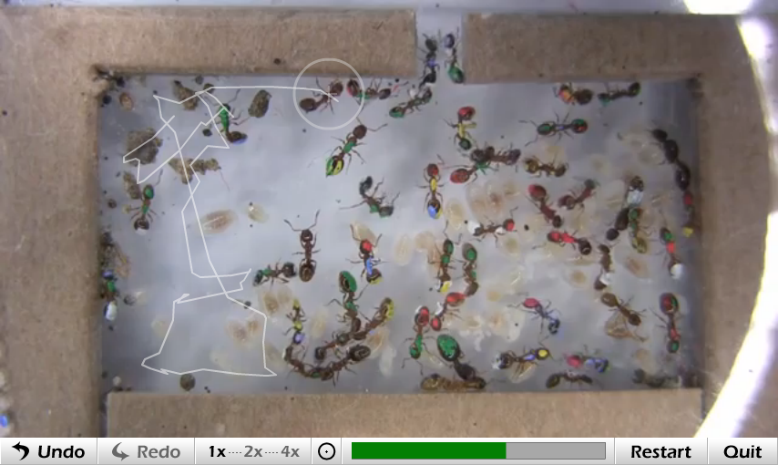
AngryAnts is our online game available at http://angryants.cs.arizona.edu, which plays videos and allows citizen scientists to build the trajectory of a specified ant via mouse clicks; see Fig. 1. When we have enough data, we compute a most realistic consensus trajectory for each ant. Our motivation comes from biologists who wish to discover longitudinal behavioral patterns in ant colonies. The trajectories of individual ants in a colony extracted from videos are needed to answer questions such as how often do ants communicate, what different roles do ants play in a colony, and how does interaction and communication affect the success or failure of a colony? Existing automated solutions are not good enough, and there is only so much data that even motivated students can annotate in the research lab.

Figure 1: A snapshot of the game environment with the selected ant in the circle.

Related Work: The problem of computing the most likely trajectory from a set of given trajectories has been studied in many different contexts and here we mention a few examples, which are similar to our approach. Buchin et al. [4] look for a representative trajectory for a given set of trajectories and compute a median representative rather than the mean. The Fréchet distance as similarity measure for trajectories is studied by Buchin et al. [3], who show how to incorporate time-correspondence and directional constraints. Trajcevski et al. [13] use the maximum distance at corresponding times as a measure of similarity between pairs of trajectories, and describe algorithms for matching under rotations and translations.

Yilmaz et al. [16] survey the state-of-the-art in object tracking methods. Some of the most recent methods include general approaches for tracking cells undergoing collisions by Nguyen et al. [11] and specific approaches for tracking insects by Fletcher et al. [6]. Also related are the automatic tracking method for tracking bees by Veeraraghavan et al. [14] and cluster-based, data-association approaches for tracking bats in infrared video by Betke et al. [2]. Tracking the motion and interaction of ants has also been studied by Khan et al. [7], who describe probabilistic methods, and by Maitra et al. [9] using computer vision techniques.

Our Contributions: We describe a citizen science approach for extracting consensus trajectories in an online game setting; see Fig. 2 for an overview. Combining human-generated trajectories with a new global approach for computing consensus curves outperforms even the most sophisticated and computationally expensive tracking algorithms [12], even in the most advantageous setting for automated solutions (e.g., high resolution video, sparse ant colony, individually painted ants).

Consider a trajectory as a sequence of $T$ pairs $(p_{i},t_{i}),1\leq i\leq T$, where $p_{i}=(x_{i},y_{i})$ is a point in the plane representing the position of an ant at timestamp $t_{i}$. We assume that between timestamps an ant keeps a constant velocity, and therefore, its trajectory is a polyline in 3D (or a possibly self-intersecting polyline in 2D). The input of our problem is a collection $\tau_{1},\dots,\tau_{m}$ of trajectories. Each trajectory corresponds to one of $k$ ants, and we assume that there exists at least one trajectory for each ant, that is, $m\geq k$. Since the input data comes from the AngryAnts game, all trajectories have the same length (number of points). We also assume that the initial position of each ant is provided by the game (from a different game level called “Count the Ants” where users click on all the ants in the first frame of the video to identify their starting positions). Therefore, the first points of trajectories corresponding to the same ant are identical. Our goal is to compute a consensus trajectory, that is, our best guess for the actual route taken, for each of the $k$ ants. While intuitively we are looking for the most probable ant trajectories, it is far from obvious how to measure the quality of a solution.

Figure 2: Overview of consensus trajectory computation via citizen science. Local consensus may route different ants along the same trajectory (red and blue), while the global consensus ensures disjoint trajectories.

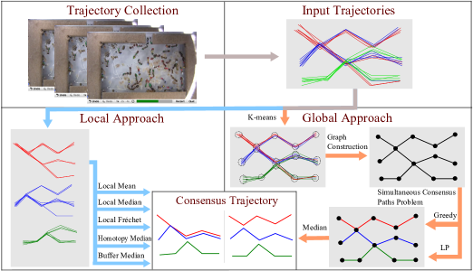
We designed, implemented, and evaluated several methods for computing accurate consensus trajectories from many (possibly inaccurate) trajectories submitted by citizen scientists. We consider several local strategies (clustering, median trajectories, and Fréchet matching) in one-ant-at-a-time setting. We also designed and implemented a novel global method in the all-ants-together setting. This approach is based on finding edge-disjoint paths in a graph constructed from all input trajectories. The underlying optimization problem is a new and interesting variant of network flow. Even though the problem is NP-complete, our two heuristics work well in practice, outperforming all other approaches including the automated system.

2 The Local Approach

Local Mean: Intuitively, a mean trajectory is the one that averages locations for input trajectories. To compute the mean, we identify all input trajectories $\tau_{1},\dots,\tau_{m_{c}}$ for a particular ant $c$. For each timestamp $t_{i}$, we query points $p_{1}=(x_{1},y_{1}),\dots,p_{m_{c}}=(x_{m_{c}},y_{m_{c}})$ corresponding to $t_{i}$. The average point is $(x_{avg},y_{avg})$, where $x_{avg}=(x_{1}+\dots+x_{m_{c}})/m_{c}$ and $y_{avg}=(y_{1}+\dots+y_{m_{c}})/m_{c}$ gives the location of the mean trajectory at timestamp $t_{i}$. The sequence of these average points over time defines the local mean consensus trajectory, which is good when the number of input trajectories is very large or when all input trajectories are very accurate. In reality, however, this is often not the case; a single inaccurate input trajectory may greatly influence the result.

Local Median: The median point is more robust to outliers than the mean. For a set of points $p_{1},p_{2},\dots,p_{m_{c}}$ the median is the point $(x_{med},y_{med})$, where $x_{med}$ is the median of the array $x_{1},\dots,x_{m_{c}}$ and $y_{med}$ is the median of the array $y_{1},\dots,y_{m_{c}}$. The sequence of these average points over time defines the local median consensus trajectory. Note that the median of a set of points is not necessarily a point of the set: it could place an ant at a point that matches none of the input trajectories.

Local Fréchet: Informally, the Fréchet distance between two trajectories can be illustrated as the minimum dog-leash distance that allows a man to walk along one trajectory and his dog along the other, while connected at all times by the leash [1]. Computing the Fréchet distance produces an alignment of the trajectories: at each step, the position of the man is mapped to the position of the dog. Given the Fréchet alignment of two trajectories, we compute their consensus by taking the midpoint of the leash over time. To find the consensus for all input trajectories, we repeatedly compute pairwise consensuses until only one trajectory remains. Since the results of the algorithm depends on the order in which the trajectories are merged, we try several different random orders choosing the best result. Note that, by definition, the Fréchet alignment of trajectories uses only the order of points and ignores the timestamps that are an essential feature of our input.

Figure 3: (a)  Simple average of trajectories may result in a consensus that goes through an obstacle. (b) The median trajectory always follows some piece of input trajectory and is robust to outliers. (c) The simple median algorithm might make a shortcut and miss a self- intersecting loop. (d) Homotopy median with an added obstacle to avoid short cutting.

Homotopy Median and Buffer Median: In the above approaches, the average of two locations could be an invalid location; see Fig. 3. In the median trajectory approaches, the computed trajectory always lies on segments of input curves; see Fig. 3. Note that this is more restrictive than the point-based median method described above. We use two algorithms suggested by Buchin et al. [4] and Wiratma [15]. In the homotopy median algorithm, additional obstacles are placed in large faces bounded by segments of input trajectories to ensure that the median trajectory is homotopic to the set of trajectories that go around the obstacles. Hence, the median does not miss segments if the input trajectories are self-intersecting; see Fig. 3 and Fig. 3. The buffer median algorithm is a combination of the buffer concept and Dijkstra’s shortest path algorithm. A buffer is defined around a segment so that if the segment is a part of the median trajectory, then its buffer intersects all input trajectories. Thus, segments located near the middle of the trajectory have smaller buffer size and are good candidates for the median trajectory. Note again that the homotopy median and buffer median approaches ignore the timestamps that are an essential feature of our input.

3 The Global Approach

In the global approach we consider all input trajectories for all $k$ ants together. The main motivation is that a trajectory corresponding to an ant may contain valid pieces of trajectories for other ants: a citizen scientist may mistakenly switch from tracking an ant $x$ to tracking a different ant $y$ at an intersection point where $x$ and $y$ cross paths. However, even when such mistakes occur, the trace after the intersection point is still useful as it contains a part of the trajectory of ant $y$. The global approach allows us to retain this possibly useful data as shown by an example in Fig. 2. Given a set of input trajectories, we compute the consensus trajectories in three steps: (1) create a graph $G$; (2) compute edge-disjoint paths in $G$; (3) extract consensus trajectories from the paths.

Step 1: We begin by creating a graph that models the interactions between ants in the video. For every timestamp, the graph has at most $k$ vertices, which correspond to the positions of the $k$ ants. If several ants are located close to each other, then we consider them to be at the same vertex. Intuitively, each such vertex is a possible point for a citizen scientist to switch to a wrong ant.

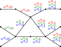
A weighted directed graph $G=(V,E)$ is constructed as follows. For every timestamp $t_{i}$, we extract points $p_{1},\dots,p_{m}$ from the given trajectories, where $p_{j}$ is the position of trajectory $\tau_{j}$ at $t_{i}$. Using a modification of the $k$-means clustering algorithm [8], we partition the points into $\leq k$ clusters. Our clustering algorithm differs from the classical $k$-means in that it always merges the points into one cluster located closer than $50$ pixels from each other. The vertices of $G$ are the clusters for all timestamps; thus, $G$ has at most $kT$ vertices. We then add edges between vertices in consecutive timestamps. Let $V_{i}$ represent a set of vertices at timestamp $t_{i}$. We add an edge $(u,v)$ between two vertices $u\in V_{i}$ and $v\in V_{i+1}$ if there is an input trajectory with point $p_{i}$ belonging to cluster $u$ and point $p_{i+1}$ belonging to cluster $v$. For each edge, we create $k$ non-negative weights. For each ant $1\leq x\leq k$ and for each edge $(u,v)\in E,u\in V_{i},v\in V_{i+1}$, there is weight $w_{uv}^{x}\in\mathbb{Z}_{\geq 0}$, which equals to the number of trajectories between timestamps $i$ and $i+1$ associated with the ant $x$ passing through the clusters $u$ and $v$.

Note that by construction graph $G$ is acyclic. Let $d^{in}(v)$ and $d^{out}(v)$ denote the indegree and the outdegree of the vertex $v$. Clearly, the only vertices with $d^{in}(v)=0$ are in $V_{1}$, and the only vertices with $d^{out}(v)=0$ are in $V_{T}$; we call them source and destination vertices and denote them by $s_{i}$ and $t_{i}$, respectively. We assume that for all intermediate vertices $v\in V_{i},1<i<T$, we have $d^{in}(v)=d^{out}(v)$; this is a realistic assumption because for each intersection point of trajectories, the number of incoming ants equals the number of outgoing ants. We say that a directed graph satisfies the ant-conservation condition if (1) the number of outgoing edges from sources and the number of incoming edges to destinations is equal to $k$, that is, $\sum_{i}d^{out}(s_{i})=\sum_{i}d^{in}(t_{i})=k$, and (2) indegree and outdegree of all its intermediate vertices are the same, that is, $d^{in}(v)=d^{out}(v)$.

Step 2: We compute $k$ edge-disjoint paths in $G$, corresponding to the most “realistic” trajectories of the ants. The paths connect the $k$ distinct vertices in $V_{1}$ to the $k$ distinct vertices in $V_{T}$. Since the initial position of each ant is a part of input, we know the starting vertex of each path. However, it is not obvious which of the destination vertices in $V_{T}$ correspond to each ant. To measure the quality of the resulting ant trajectories, that is, how well the edge-disjoint paths match the input trajectories, we introduce the following optimization problem.

Simultaneous Consensus Paths (SCP)
Input: A directed acyclic graph $G=(V,E)$ with $k$ sources $s_{1},\dots,s_{k}$ and $k$ destinations $t_{1},\dots,t_{k}$ satisfying the ant-conservation condition. The weight of an edge $e\in E$ for $1\leq i\leq k$ equals $w_{e}^{i}\in\mathbb{Z}_{\geq 0}$.
Task: Find $k$ edge-disjoint paths $P_{1},\dots,P_{k}$ so that path $P_{i}$ starts at $s_{i}$ and ends at $t_{j}$ for some $1\leq j\leq k$, and the total $cost=\sum_{i=1}^{k}\sum_{e\in P_{i}}w_{e}^{i}$ is maximized. Note that the objective is to simultaneously optimize all $k$ disjoint paths. The decision problem is to find $k$ edge-disjoint paths with total $cost\geq c$ for some constant $c\geq 0$.

The problem is related to the integer multi-commodity flow problem, which is known to be NP-hard [5]. In our setting, the weights on edges for different “commodities” are different, and the source-destination pairs are not known in advance. We study the SCP problem in the next section.

Step 3: We construct consensus trajectories corresponding to a solution of the SCP problem. Let $P$ be a path for an ant $x$ computed in the previous step. For each timestamp $t_{i}$, we consider the edge $(u,v)\in P,u\in V_{i},v\in V_{i+1}$, and find a set $S_{uv}$ of all input trajectories passing through both clusters $u$ and $v$. We emphasize here that $S_{uv}$ may contain (and often does contain) trajectories corresponding to more ants than just ant $x$. Next we compute the median of points of $S_{uv}$ at timestamp $t_{i}$; the median is used as the position of ant $x$ at timestamp $t_{i}$. The resulting trajectory of $x$ is a polyline connecting its positions for all $t_{i},1\leq i\leq T$.

4 The Simultaneous Consensus Paths Problem

The SCP problem is NP-complete even when restricted to planar graphs by a reduction from a variant of the edge-disjoint path problem [10]. On the other hand, the problem is fixed-parameter tractable in the number of paths. For a fixed constant $k$, it can be solved optimally via dynamic programming in time $O(|E|+k!|V|)$.

4.1 Hardness Result

Let a grid graph be one that is a subgraph of the rectangular grid, that is, a graph with $n\times m$ vertices such that $v_{i,j}$ is connected to $v_{i^{\prime},j^{\prime}}$ if and only if $|i-i^{\prime}|=1$ and $j=j^{\prime}$, or $i=i^{\prime}$ and $|j-j^{\prime}|=1$. It is easy to see that any grid graph is planar. We prove that the SCP problem is NP-complete even when restricted to grid graphs by a reduction from a variant of the edge-disjoint path problem, which is formulated as follows.

Disjoint Paths
Input: A directed acyclic grid graph $G$ satisfying the ant-conservation condition and a set of $k$ source-destination pairs $(s_{1},t_{1}),\dots,(s_{k},t_{k})$.
Task: Find $k$ edge-disjoint paths $P_{1},\dots,P_{k}$ so that $P_{i}$ starts at $s_{i}$ and ends at $t_{i}$.

There are two differences with the SCP problem: (1) in the Disjoint Paths problem, a source-destination pair is fixed for every path; (2) the goal is to construct $k$ paths, while the SCP problem is an optimization of a weighted sum. Deciding whether the Disjoint Paths problem has a solution with exactly $k$ paths is NP-complete [10]. We also note that the graphs used in the construction of the proof satisfy the ant-conservation condition.

Theorem 4.1

The SCP problem is NP-complete on acyclic directed grid graphs.

Proof

It is easy to verify a solution of SCP in polynomial time; we argue the hardness result via standard reduction. Let $G=(V,E)$, $(s_{1},t_{1}),\dots,(s_{k},t_{k})$ be an instance of the Disjoint Paths problem. We create a new directed acyclic graph $G^{\prime}$ satisfying the ant-conservation condition. Then we assign weights for the edges of $G^{\prime}$ so that an optimal solution for the SCP problem on $G^{\prime}$ connects as many pairs $(s_{i},t_{i})$ as possible. $G^{\prime}$ is constructed from $G$ by adding extra $k$ sources and $k$ paths of length $k|V|$, which we refer to as tails; see Fig. 4. In the new graph $V^{\prime}=V\cup\{s_{1}^{\prime},\dots,s_{k}^{\prime}\}\cup T_{1}\cup\dots\cup T_{k}$, where every tail $T_{i}=\{t_{i_{1}},t_{i_{2}},\dots,t_{i_{k|V|}}=t_{i}^{\prime}\}$. Edges in $G^{\prime}$ connect the new sources and the tails with the vertices of $G$:

$$E^{\prime}=E\cup\bigcup_{i=1}^{k}(s_{i}^{\prime},s_{i})\cup\bigcup_{i=1}^{k}\{(t_{i},t_{i_{1}}),(t_{i_{1}},t_{i_{2}}),\dots,(t_{i_{k|V|-1}},t_{i_{k|V|}})\}.$$

Every maximal path (in terms of edges) in $G^{\prime}$ has its dedicated source, and no two edge-disjoint paths end at the same destination. It is easy to see that $G^{\prime}$ is acyclic and satisfies the ant-conservation condition.

In the SCP problem, the paths do not have fixed destinations. To make sure that a path starts at $s_{i}^{\prime}$ and ends at $t_{i}^{\prime}$, assign heavy weights to the edges on the tail of the $i$-th path: For every $1\leq i\leq k$, choose some path $R_{i}$ from $s_{i}^{\prime}$ to $t_{i}^{\prime}$. For all edges $e\in R_{i}$, set $w^{i}_{e}=1$, and for the remaining edges, $e\not\in R_{i}$, set $w^{i}_{e}=0$. Note that these paths $R_{i}$ need not be disjoint; we use them only to assign the edge weight; see Fig. 4.

Figure 4: (a) The input grid graph $G$ for the Disjoint Paths problem with 3 source-destination pairs. (b) Construction of the graph $G^{\prime}$. Paths $R_{1}$, $R_{2}$, and $R_{3}$ are colored red (solid), green (dotted), and blue (dashed), respectively. The tail connecting $t_{i}$ with $t_{i}^{\prime}$ for $1\leq i\leq 3$ forces a path $P_{i}$ to end at $t_{i}$ in the optimal solution of the SCP problem.

Now we prove that there are $k$ edge-disjoint paths in $G$ if and only if there is a solution of the SCP problem for $G^{\prime}$ with $cost\geq k^{2}|V|$. If there exist $k$ edge-disjoint paths in $G$ connecting $s_{i}$ to $t_{i}$, then we can use these paths to construct heavy paths in $G^{\prime}$. Let $P_{i}=s_{i}\dots t_{i}$ be a path in $G$. Path $P_{i}^{\prime}$ is constructed from $P_{i}$ by adding a source and a tail: $P_{i}^{\prime}=s_{i}^{\prime}s_{i}\dots t_{i}\dots t_{i}^{\prime}$. Since $w^{i}_{e}=1$ for the edges $e$ than $k|V|$. Paths $P_{i}^{\prime}$ form a solution for the problem with $cost\geq k^{2}|V|$.

Conversely, suppose the edge-disjoint paths $P_{i}^{\prime}$ are a solution for the SCP problem with $cost\geq k^{2}|V|$. We show that every $P_{i}^{\prime}$ passes through $s_{i}$ and $t_{i}$ and, therefore, subpaths $P_{i}=P_{i}^{\prime}\cap V$ (a subgraph of $P_{i}^{\prime}$ induced by $V$) comprise a solution for the Disjoint Paths problem. For the sake of contradiction, suppose $P_{i}^{\prime}$ does not pass through $t_{i}$, that is, it ends at $t_{j}^{\prime}$ for some $j\neq i$. Then $P_{i}^{\prime}$ passes through the “wrong tail”: $P_{i}^{\prime}=s_{i}^{\prime}s_{i}\dots t_{j}\dots t_{j}^{\prime}$. The weight of $P_{i}^{\prime}$ is at most $|V|$ since there are at most $V$ edges in $E$ with weight $w^{i}_{e}=1$. Symmetrically, path $P_{j}^{\prime}$ has weight at most $|V|$. Since the maximum weight on edges of $E$ is $k|V|$, the paths $P_{i}^{\prime}$ have weight at most $k|V|+k(k-2)|V|<k^{2}|V|$, thus contradicting our assumption.

4.2 Exact Algorithm for Few Paths

The next theorem implies that the SCP problem is fixed-parameter tractable in the number of paths. Note that if a graph $G$ satisfies the ant-conservation condition, then in any solution with $k$ edge-disjoint paths all the edges of $G$ are covered by a path [10].

Theorem 4.2

For a fixed constant $k$, the SCP problem can be solved optimally in time $O(|E|+k!|V|)$.

Proof

Let $G=(V,E)$ be the input directed acyclic weighted graph, $s_{1},\dots,s_{k}\in V$ be the sources, and $t_{1},\dots,t_{k}\in V$ be the destinations. We solve the problem using dynamic programming. First, we compute a topological order of the vertices of $G$ and fix the resulting order $u_{1},\dots,u_{|V|}$. For convenience, we add a super-destination vertex $t$ to $G$ together with zero-weight edges $(t_{1},t),\dots,(t_{k},t)$. Let $G^{i}=(V^{i},E^{i})$ for $1\leq i\leq|V|+1$ be a subgraph of $G$ induced by the vertices $u_{i},\dots,u_{|V|},t$. For each $0\leq i\leq|V|+1$ we construct a multiset $T_{i}$ with $|T_{i}|=k$. The multiset $T_{0}$ consists of sources of $G$ so that $s_{i}$ is present $d^{out}(s_{i})$ times. For every $1\leq i\leq|V|$, we build $T_{i+1}$ from $T_{i}$ by removing vertex $u_{i}$ and adding its outgoing neighbors. It easy to see that $T_{|V|+1}=(t,\dots,t)$.

Let us call the state corresponding to $V^{i}$ an ordered sequence of elements (not necessarily distinct) of $T_{i}$; that is, $(v_{1},\dots,v_{k})$ in which $v_{j}\in T_{i},1\leq j\leq k$ for some $i$. For a state $(v_{1},\dots,v_{k})$, let $F(v_{1},\dots,v_{k})$ be the optimal cost of routing $k$ edge-disjoint paths on $G$ so that the $i$-th path starts at $v_{i}$ and ends at $t$. It is easy to see that $F(t,\dots,t)=0$, and the optimal solution for the SCP problem is $F(s_{1},\dots,s_{k})$.

In order to compute the value $F(S)$ for the state $S=(v_{1},\dots,v_{k})$ corresponding to $V^{i}$, we choose the vertex $u_{i}\in S$. Consider the edges $e_{1}=(u_{i},a_{1}),\dots,e_{d}=(u_{i},a_{d})$, where $d=d^{out}(u_{i})$. Since all these edges should be covered by paths, the vertex $u_{i}$ is repeated exactly $d^{in}(u_{i})=d$ times in $S$; without loss of generality we may assume that $S=(u_{i},\dots,u_{i},v_{d+1},\dots,v_{k})$. The paths may cover the edges in $d!$ different ways:

$$F(v_{1},\dots,v_{d},v_{d+1},\dots,v_{k})=\max_{\pi}\left(F(a_{\pi_{1}},\dots,a_{\pi_{d}},v_{d+1},\dots,v_{k})+\sum_{j=1}^{k}w^{\pi_{j}}_{e_{j}}\right),$$

where $\pi$ runs over all permutations of $\{1,\dots,d\}$. Note that $(a_{\pi_{1}},\dots,a_{\pi_{d}},v_{d+1},\dots,v_{k})$ is a state corresponding to $T_{j}$ with $j=i+1$.

The correctness of the algorithm follows from the observation that we consider all possible ways to route the paths at every intermediate vertex. The number of different states corresponding to $V^{i}$ is $k!/d!$, where $d$ is the outdegree of the vertex $u_{i}$. In order to compute the values $F(S)$ for a state corresponding to $V^{i}$ we check $d!$ permutations; hence, the running time is $k!$ for each $V^{i}$. Summing over all graphs $G_{i}$, we obtain $O(|E|+k!|V|)$ running time.

Next we suggest a greedy heuristic and provide an integer linear programming (ILP) formulation for SCP.

Figure 5: The greedy algorithm may produce non-optimal solution. (a) The input graph with 3 paths: R, G, and B. (b) The paths computed by the greedy algorithm with $cost=75$ (R is shown solid, G – dotted, B – dashed). (c) The optimal solution with $cost=77$.

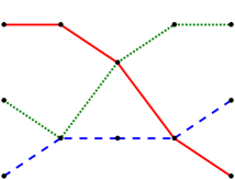
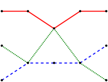
The Greedy Algorithm: The algorithm finds the longest path among all source-destination pairs $s_{i}$, $t_{j}$. The length of a path starting at $s_{i}$ is the sum of $w^{i}_{uv}$ for all edges $(u,v)$ of the path. Since $G$ is an acyclic directed graph, the longest path for the specified pair $s_{i},t_{j}$ can be computed in time $O(|E|+|V|)$ via dynamic programming. Once the longest path is found, we remove all edges of the path from $G$ and proceed with the next longest path. The algorithm finds at most $k$ paths on each iteration and the number of iterations is $k$; hence, the overall running time is $O(k^{2}(|V|+|E|))$.

The algorithm always yields a solution with $k$ disjoint paths. Initially, $G$ satisfies the ant-conservation condition: $d^{in}(v)=d^{out}(v)$ for all intermediate vertices $v$. Since $G$ is connected, there exists a source-destination path. After removing the longest path, $G$ may be disconnected, but the ant-conservation condition still holds for every connected component. The number of outgoing edges from sources and the number of incoming edges to destinations are equal for every connected component. Thus, the greedy algorithm produces a feasible solution but not necessarily the optimal one; see Fig. 5.

Figure 6: Graph in which a fractional solution has cost greater than the cost of any integer solution. (a) The input graph with 4 paths. The vector on the edge $e$ corresponds to the weights $(w_{e}^{1},w_{e}^{2},w_{e}^{3},w_{e}^{4})$ for the paths on $e$. (b) The optimum integer solution with $cost=15$. The vector on the edge $e$ corresponds to the solution $(x_{e}^{1},x_{e}^{2},x_{e}^{3},x_{e}^{4})$ on $e$. (c) A fractional solution with $cost=16$. The vector on the edge $e$ corresponds to the solution $(x_{e}^{1},x_{e}^{2},x_{e}^{3},x_{e}^{4})$ on $e$.

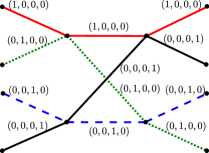
Linear Programming Formulation: Let $P_{i}$ denote the path in $G$ from $s_{i}$ to $t_{j}$ for some $j$ (the path of the $i$-th ant). For each $P_{i}$ and each edge $e$, we introduce a binary variable $x_{e}^{i}$, which indicates whether path $P_{i}$ passes through the edge $e$. The SCP problem can be formulated as the following ILP:

$$\begin{array}[]{llcllr}\mbox{{maximize}}&\sum_{e}\sum_{i}w_{e}^{i}x_{e}^{i}\\ \mbox{{subject to }}&\sum_{i}x_{e}^{i}&=&1&\forall e\in E&\>\>\>\>(1)\\ &\sum_{uv}x_{uv}^{i}&=&\sum_{vw}x_{vw}^{i}&\forall v\in V\setminus\{s_{1},t_{1},\ldots,s_{k},t_{k}\},1\leq i\leq k&(2)\\ &\sum_{v}x_{s_{i}v}^{i}&=&1&\forall 1\leq i\leq k&(3)\\ &x_{e}^{i}&\in&\{0,1\}&\forall e\in E,1\leq i\leq k&(4)\end{array}$$

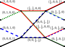
Here constraint (1) guarantees that the paths are disjoint: there is exactly one path passing through every edge. Constraint (2) enforces consistency of the paths at every intermediate vertex: if a vertex $v$ is contained in a path, then the path passes through an edge $(u,v)$ and an edge $(v,w)$ for some $u,w\in V$. In constraint (3) we sum over vertices $v$ with $(s_{i},v)\in E$; it implies that the $i$-th path starts at source $s_{i}$. If we relax the integrality constraint (4) by $0\leq x_{e}^{i}\leq 1$, we have a fractional LP formulation for the SCP problem, which can be solved in polynomial-time. However, the solution does not have a natural interpretation in the context of ants (fractional ants do not make sense in the biological problem). Further, we found an example for which the best fractional solution has cost strictly greater than the cost of any integer solution; see Fig. 6.

We can convert an optimal fractional LP solution $x^{*}$ into a feasible integer solution as follows. Randomly pick an ant $1\leq i\leq k$, with probability of choosing the $i$-th ant proportional to its weight $\sum_{e}w_{e}^{i}{x^{*}}_{e}^{i}$ in the fractional solution. We then consider the graph with modified edge weights in which the weight of an edge $e\in E$ is $w_{e}^{i}{x^{*}}_{e}^{i}$. We look for the longest path starting at source $s_{i}$ in this graph, assign the path to the $i$-th ant, and remove this path from the graph. We then rerun the LP to find a fractional solution on the smaller instance. Our experiments suggest that this rounding scheme yields an integer solution that is close to optimal.

5 Experimental Results

We use a machine with Intel i5 3.2GHz, 8GB RAM and CPLEX Optimizer.

Table 1: Average and worst root-mean-square error (in pixels) computed for proposed algorithms.

Algorithm	Worst RMSE	Average RMSE	Runtime
Automated Solution	95.308	9.593	$160$ min
Local Mean	105.271	12.531	$<100$ ms
Local Median	112.741	9.801	$<100$ ms
Local Fréchet	127.104	15.562	$1.2$ sec
Homotopy Median	146.267	20.244	$8.2$ sec
Buffer Median	171.556	23.998	$9.7$ sec
Global ILP	20.588	8.716	$34$ sec
Global Greedy	24.820	8.900	$0.2$ sec

Real-World Dataset: Here we consider a real-world scenario and compare ground truth data to seven different consensus algorithms described in this paper, along with an automated solution. To evaluate our various algorithms, we work with a video of a Temnothorax rugatulus ant colony containing $10,000$ frames, recorded at $30$ frames per second. This particular video contains ants that are individually painted and has been analyzed with the state-of-the-art automated multi-target tracking system of Poff et al. [12]. The method required about $160$ minutes to analyze the video. To evaluate the automated system, they create a ground truth trajectory for each ant, by manually examining every ant in every 100th frame of the automated output and correcting when necessary. We use this ground truth data to evaluate the efficiency of the algorithms considered and the automated system. Note that just by the way the ground truth is generated, results are inherently biased in favor of the automated solution.

Our dataset consists of $252$ citizen scientist generated trajectories for $50$ ants, with between $2$ and $8$ trajectories per ant. To compute the ant trajectories, we construct the interaction graph $G$, as described in Section 3. For our dataset, the graph contains $4,246$ vertices and $10,494$ edges. We apply the five local methods and two of the global methods (greedy and integer linear programming) to build consensus trajectories.

We computed seven different consensus trajectories for each ant: five based on the local algorithms, and two based on the global algorithms. An overview of results is in Table 1 and in Fig. 8. We compare all seven, as well as the trajectories computed by the automated system, by measuring average and worst root-mean-square error of the Euclidean distance between pairs of points of computed and ground truth trajectories. We notice that the approximate dimensions of an ant in our video are $60\times 15$ pixels.

Among the local approaches, the local median is best. The local mean is negatively impacted by the outliers in the data. The Fréchet approach, Homotopy median, and Buffer median perform poorly. This could be due to the very self-intersecting trajectories making these algorithms miss entire pieces. We used the default values for all the parameters in these algorithms; a careful tuning will likely improve accuracy. In the Fréchet approach we tried $50$ different random orders of merging trajectories.

Figure 7: (a) The automated solution (red) switches to the wrong ant, while our local median consensus (green) agrees the majority of input trajectories (black). (b) Most of the input trajectories (black) follow the wrong ant; hence, the local median consensus (green) is incorrect. Here our global consensus trajectory (dark blue) finds a trajectory closer to the ground truth (pink).

Figure 8: (a) Root-mean-square error for the 10 “most movable” ants (according to the ground truth). (b) Comparison of tracking accuracy between automated solution and proposed algorithms.

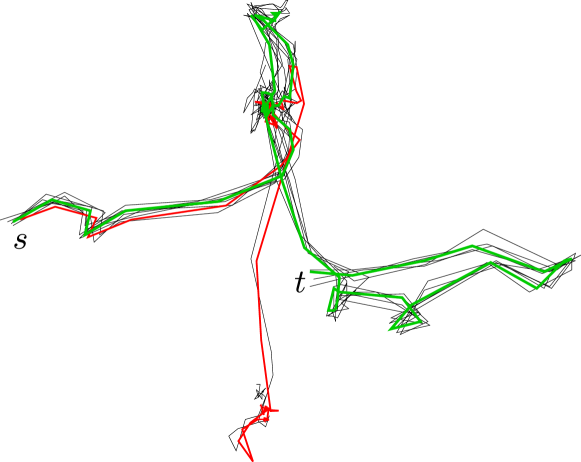
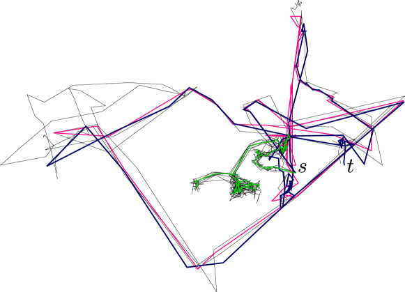
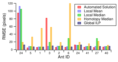
The two global approaches perform similarly. There are only few segments of trajectories where the results differ. It is important to emphasize here the cases where the citizen scientists make the same mistake do happen in practice. We found an example in which 5 out of 8 input trajectories follow the wrong ant; see Fig. 7. In this case, none of the local algorithms have a chance to recover a correct trajectory. Only the global approaches allow us to identify the correct ant and produce the most accurate results. We stress again that the ground truth data is inherently biased towards the automated solution because it was obtained by modifying the trajectories obtained from the automated solution. Yet our global algorithms perform better.

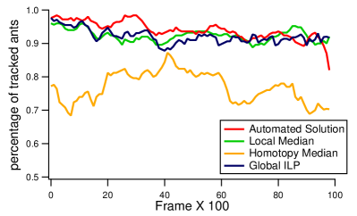
A big challenge for the existing automated systems is tracking ants in long videos. For long videos (e.g., hundreds or even thousands of hours), automated tracking methods are not reliable. Whenever such algorithms loose tracking, the error quickly accumulates and a trajectory often is not recovered; see Fig. 7. Our global approaches naturally resolve this problem. We evaluate tracking accuracy as the percentage of ants correctly “tracked” at a given timestamp; here, we consider the ant correctly tracked if the distance between the ground truth and our trajectory is less than 15 pixels (typical width of ant head). The accuracy of the automated solution decreases over time, and by the end of the 5-minute video it is below $87\%$ accuracy; see Fig. 8. Our algorithms are steadily over $90\%$ accuracy over the entire video.

Synthetic Dataset: In order to validate our global approach on a larger dataset, we generate a collection of synthetic graphs. Here we test our algorithms for the SCP problem, that is, the algorithms for computing disjoint paths on graphs, rather than for extracting optimal trajectories. We construct a set of directed acyclic graphs having approximately the same characteristics as the interaction graph computed for the real-world dataset. The graph construction follows the same pipeline as described in Section 3; every graph is generated for $k\leq 50$ ants and $T\leq 100$ timestamps. The ants form $k$ vertices for the initial timestamp; on every subsequent timestamp pairs of ants meet with probability $0.4$ (the constant estimated for the real-world graph). Thus, for every timestamp, we have from $k/2$ to $k$ vertices. The pairs of ants meeting at a timestamp are chosen randomly with the restriction that indegrees and outdegrees of every vertex in a graph are equal and at most $2$. By construction of the graphs, we naturally get “ground truth” paths for all ants. Next we generate citizen scientist trajectories in two scenarios: $2-8$ trajectories (as in the real-world dataset) and $15-20$ trajectories per ant. A citizen scientist tracking an ant is modeled by a path starting at the source of the ant. At every junction vertex (with outdegree $2$) there is fixed probability $P(error)$ of making a mistake by switching from tracking the current ant to the other one. If $P(error)=0$, then user trajectories always coincide with the ground truth paths; if $P(error)=0.5$, the trajectories may be considered as random walks on the graph.

Figure 9: Precision of the algorithms on the synthetic dataset. Solid lines represent average values over $5$ runs of the algorithms for a given error/timestamp. (a) Results for $k=50$ ants, $T=100$ timestamps (5-minute video segment), and various values of $P(error)$. (b) Results for $k=50$ ants, $2-8$ user trajectories per ant, and various number of timestamps.

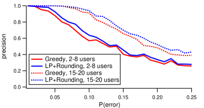
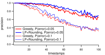
We evaluate the greedy heuristic (Greedy) and the linear program with rounding (LP+Rounding). As the latter heuristic is a randomized algorithm, we report the best result over $5$ runs for a given input. For small instances, we also compute an exact solution using the integer linear program (ILP). We analyze the precision of the algorithms under various parameters. For every edge of the graph $G$, we say that it is correctly identified if both the algorithm and the ground truth assign the edge to the same path. The precision is measured as the fraction of correctly identified edges in $G$: a value of $1$ means that all paths are correct. As in the real-world dataset, we consider a scenario with $k=50$ ants. As expected, increasing the probability of making a mistake decreases the quality of the solution; see Fig. 9. However, increasing the number of user trajectories does help. Both algorithms recover all paths correctly if the number of trajectories for each ant is more than $15$, even in a case with $P(error)=0.1$. On the other hand, with $P(error)>0.2$ the precision drops to under $50\%$. Although we cannot definitively measure the accuracy of all citizen scientists, empirical evidence from our experiment indicates that the error rate was very low: $P(error)=0.02$. This is an order of magnitude lower than the upper limit on errors that our algorithms can handle. We also consider the impact of video length on the precision of the algorithms; see Fig. 9. Not surprisingly, precision is higher for short videos: for $2$-minute segments ($40$ timestamps) and $P(error)=0.05$, LP+Rounding produces the correct paths, while for $5$-minute segments ($100$ timestamps) only $60\%$ of paths are correct.

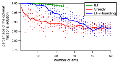
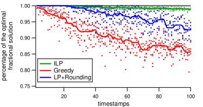
We also analyze the effectiveness of the Greedy and LP+Rounding algorithms for the SCP problem with $P(error)=0.2$ and $2-8$ trajectories per ant; see Fig. 10. To normalize the results, values are given as a percentage of the $cost$ of an optimal fractional solution (FLP) for the SCP problem. Note that the ILP results are in the range$[0.98,1.0]$, which means that an optimal integer solution is always very close to the optimal fractional solution. Both Greedy and LP+Rounding perform very well, achieving $\approx 0.85$ of the optimal solution. These two algorithms produce similar results, with LP+Rounding usually outperforming Greedy.

Figure 10: Quality of the algorithms: ratio between the $cost$ of obtained solution and the optimal (fractional) $cost$. Results for single instances are depicted by dots and solid curves show the average values over $5$ runs for a given number of ants/timestamps. Note that the y-axis starts at value $0.75$. (a) Results for $T=100$ timestamps, $P(error)=0.2$, and $2-8$ user trajectories per ant. (b) Results for $k=20$ ants, $P(error)=0.2$, and $2-8$ user trajectories per ant.

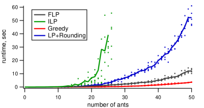
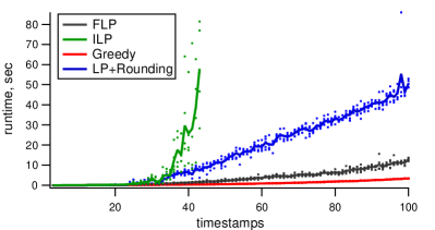
Running times are shown in Fig. 11. As expected, the greedy algorithm, with complexity dependent linearly on the size of the graph, finishes in under few milliseconds. The ILP is also relatively quick on the real-world dataset, computing the optimal solution within a minute. On synthetic data and more erroneous real-world data the ILP approach is applicable only when the number of ants is small, e.g., $k<25$. For larger values of $k$, the computation of optimal disjoint paths takes hours. On the other hand, LP+Rounding is fast: the real-world instances with $k=50$ ants and $T=100$ timestamps are processed within a minute. Greedy takes only $2-3$ seconds on the largest instances and may be used in an online fashion. We conclude that the running times of all of our algorithms (except ILP) are practical.

6 Conclusions and Future Work

We described a system for computing consensus trajectories from a large number of input trajectories, contributed by untrained citizen scientists. We proposed a new global approach for computing consensus trajectories and experimentally demonstrated its effectiveness. In particular, the global approach outperforms the state-of-the-art in computer vision tools, even in their most advantageous setting (high resolution video, sparse ant colony, individually painted ants). In reality, there are hundreds of thousands of hours of video in settings that are much more difficult for the computer vision tools and where we expect our citizen science approach to compare even more favorably.

A great deal of challenging problems remain. Arguably, the best method would be to track “easy ants” and/or “easy trajectory segments” automatically, while asking citizen scientists to solve the hard ants and hard ant trajectory segments. In such a scenario, every input trajectory will describe a part of the complete ant trajectory, which would require stitching together many short pieces of overlapping trajectories.

Figure 11: Running time of the algorithms with $P(error)=0.2$ and $2-8$ trajectories per ant. The results for single instances are depicted by dots, while solid lines represent average values over $5$ runs for a given number of ants/timestamps. (a) Results for $T=100$ timestamps and various number of ants. (b) Results for $k=50$ ants and various length of a video.

Acknowledgments. We thank the A. Dornhaus lab for introducing us to the problem, and M. Shin and T. Fasciano for automated solutions and ground truth. We thank A. Das, A. Efrat, F. Brandenburg, K. Buchin, M. Buchin, J. Gudmundsson, K. Mehlhorn, C. Scheideler, M. van Kreveld, and C. Wenk for discussions. Finally, we thank J. Chen, R. Compton, Y. Huang, Z. Shi, and Y. Xu for help with the game development.

References

- [1] Alt, H., Godau, M.: Computing the Fréchet distance between two polygonal curves. Internat. J. Comput. Geom. Appl. 5(1), 75–91 (1995)
- [2] Betke, M., Hirsh, D., Bagchi, A., Hristov, N., Makris, N., Kunz, T.: Tracking large variable numbers of objects in clutter. In: CVPR. pp. 1–8. IEEE Computer Society, Washington (2007)
- [3] Buchin, K., Buchin, M., Gudmundsson, J.: Constrained free space diagrams: a tool for trajectory analysis. Int. J. Geogr. Inf. Sci. 24(7), 1101–1125 (2010)
- [4] Buchin, K., Buchin, M., Kreveld, M., Löffler, M., Silveira, R., Wenk, C., Wiratma, L.: Median trajectories. Algorithmica 66(3), 595–614 (2013)
- [5] Even, S., Itai, A., Shamir, A.: On the complexity of timetable and multicommodity flow problems. SIAM J. Comput. 5(4), 691–703 (1976)
- [6] Fletcher, M., Dornhaus, A., Shin, M.: Multiple ant tracking with global foreground maximization and variable target proposal distribution. In: WACV. pp. 570–576. IEEE Computer Society, Washington (2011)
- [7] Khan, Z., Balch, T., Dellaert, F.: MCMC-based particle filtering for tracking a variable number of interacting targets. IEEE TPAMI 27(11), 1805–1819 (2005)
- [8] Lloyd, S.: Least squares quantization in PCM. IEEE Trans. Inf. Theory 28(2), 129–137 (1982)
- [9] Maitra, P., Schneider, S., Shin, M.: Robust bee tracking with adaptive appearance template and geometry-constrained resampling. In: WACV. pp. 1–6. IEEE Computer Society, Washington (2009)
- [10] Marx, D.: Eulerian disjoint paths problem in grid graphs is NP-complete. Discrete Appl. Math. 143(1-3), 336–341 (2004)
- [11] Nguyen, N., Keller, S., Norris, E., Huynh, T., Clemens, M., Shin, M.: Tracking colliding cells in vivo microscopy. IEEE Trans. Biomed. Eng. 58(8), 2391–2400 (2011)
- [12] Poff, C., Hoan, N., Kang, T., Shin, M.: Efficient tracking of ants in long video with GPU and interaction. In: WACV. pp. 57–62. IEEE Computer Society, Washington (2012)
- [13] Trajcevski, G., Ding, H., Scheuermann, P., Tamassia, R., Vaccaro, D.: Dynamics-aware similarity of moving objects trajectories. In: GIS. pp. 1–8. ACM, New York (2007)
- [14] Veeraraghavan, A., Chellappa, R., Srinivasan, M.: Shape-and-behavior encoded tracking of bee dances. IEEE TPAMI 30(3), 463–476 (2008)
- [15] Wiratma, L.: Following the Majority: A New Algorithm for Computing a Median Trajectory. Master’s thesis, Dept. of Information and Computing Sciences, Utrecht University (2010)
- [16] Yilmaz, A., Javed, O., Shah, M.: Object tracking: a survey. ACM Comput. Surv. 38, 1–45 (2006)