Phase transition of light on complex quantum networks

Abstract

Recent advances in quantum optics and atomic physics allow for an unprecedented level of control over light-matter interactions, which can be exploited to investigate new physical phenomena. In this work we are interested in the role played by the topology of quantum networks describing coupled optical cavities and local atomic degrees of freedom. In particular, using a mean-field approximation, we study the phase diagram of the Jaynes-Cummings-Hubbard model on complex networks topologies, and we characterize the transition between a Mott-like phase of localized polaritons and a superfluid phase. We found that, for complex topologies, the phase diagram is non-trivial and well defined in the thermodynamic limit only if the hopping coefficient scales like the inverse of the maximal eigenvalue of the adjacency matrix of the network. Furthermore we provide numerical evidences that, for some complex network topologies, this scaling implies an asymptotically vanishing hopping coefficient in the limit of large network sizes. The latter result suggests the interesting possibility of observing quantum phase transitions of light on complex quantum networks even with very small couplings between the optical cavities.

I Introduction

Quantum optics and atomic physics have reached a level of control over light-matter interactions which not only makes it feasible the emulation of condensed matter models Plenio ; Plenio2 , but also inspires new architectures envisaging a future quantum Internet with a desired topology QI ; Ritter . Hence the potential advantage coming from a combined optical and atomic approach is twofold: on one hand, being able to control a quantum system that simulates another one is a way to realize a special purpose quantum computer; on the other hand, the possibility of manipulating new degrees of freedom (not accessible in condensed matter systems) motivates the experimental and theoretical study of new quantum systems, with the possibility of discovering new physical phenomena. In this respect an important outcome, coming from the combined experimental investigations of atomic and optical systems, is the realization of coupled cavity arrays interacting with local atomic degrees of freedom Plenio . These systems allow for the controlled interaction between trapped atoms and local cavity photons, and moreover photons are free to hop between coupled cavities. Changing the details of the physical setup different many-body models can be realized Plenio ; Schiro , and one in particular is of interest in the present work: the Jaynes-Cummings-Hubbard (JCH) model Jaynes ; Greentree ; Greentree2 ; LeHur ; Vuckovic ; Blatter ; Pelster . Part of the interest in these systems is motivated by the possibility to investigate new quantum critical phenomena Sachdev , like the quantum phase transition of light between a Mott-like regime and a superfluid phase Jaynes ; Greentree ; Greentree2 ; LeHur ; Vuckovic ; Blatter ; Pelster . Also of interest is the possibility to generate quantum simulators that naturally access non-equilibrium physics Koch .

In this work we are interested in an additional degree of freedom which optical arrays can provide, i.e. the topology of the network underlying the quantum dynamics. While regular lattice structures with short-range interactions are the typical framework in standard quantum emulator architectures, fiber-coupled cavities may allow for the realization of quantum networks with distant effective interactions between local degrees of freedom Ritter ; Zheng ; Kyoseva . These effective long-range interactions are an important ingredient for the construction of quantum networks with complex topology, which is a recent topic of interest in the quantum information and complex network community Ranking_Silvano1 ; Ranking_Silvano2 ; Ranking_Jesus ; Jesus_Entaglement ; Burioni_BEC ; Havlin_localization_1 ; Havlin_localization_2 ; Hubbard_Apollonian ; Free_Electron_Gas_Apollonian ; Bose_Einstein_Apollonian ; QTIM ; JSTAT ; BH ; Severini ; entropy_silvano . Along this line of research, in this work we study the effect of the array topology on the phase diagram of the JCH model. Motivations come not only from the possible experimental realization of such systems, but also from a number of results, especially in the classical context, underlying the importance of networks’ topologies. Indeed for classical systems it is well known that the topology of the network can significantly change the phase diagram of some models, and their critical behavior crit ; Dynamics . On the quantum side previous results on the Bose-Hubbard model Fisher ; Greiner ; Inguscio ; Vezzani ; Laser are particularly inspiring for the present work. In fact, for this model, it has been shown by mean-field arguments that the phase diagram depends of the maximal eigenvalue $\Lambda$ of the hopping matrix describing the topology of the network BH ; Laser . This result is valid both in presence of disorder Laser and in presence of a complex topology BH . Interestingly in a complex random network topology, or in an Apollonian network Apollonian1 ; Apollonian2 , the maximal eigenvalue of the adjacency matrix diverges with the network size. In BH it has been shown, for the Bose-Hubbard model, that this divergence implies a non-trivial scaling of the hopping coefficient, in order to not suppress the Mott-insulator phase in the thermodynamic limit.

Here we consider instead the properties of the JCH model on complex quantum network topologies. Using mean-field theory we characterize the phase diagram of the model at $T=0$, which presents a phase transition between a Mott-like regime and a superfluid phase. We demonstrate analytically, and confirm numerically, that the phase diagram is non-trivial and well defined only if the hopping coefficient $\kappa$ scales as the inverse of the maximal eigenvalue $\Lambda$ of the hopping matrix, i.e. $\kappa\propto\frac{1}{\Lambda}$. Furthermore we characterize the scaling of the maximal eigenvalue for a number of well known complex network topologies, showing that in many cases the maximal eigenvalue $\Lambda$ diverges with the network size $N$. Therefore our results are of general interest for a number of different complex topologies, and they imply that for complex network arrays interesting quantum critical behaviors can be observed even with very small couplings between different cavities.

The rest of the paper is organized as follows: in Sec. II we introduce the Jaynes-Cummings Hamiltonian and some of its properties; in Sec. III we characterize the Jaynes-Cummings-Hubbard model, its mean-field solution, and we consider the scaling behavior of the hopping coefficient for different network topologies; Sec. IV is devoted to discussions and conclusions. In the Appendix a detailed derivation of the mean field solution is provided.

II Atom-Photon interaction in a single cavity

The standard model describing the interaction between a two-level atom and quantized electromagnetic modes is provided by the Jaynes-Cummings Hamiltonian. In the rotating wave approximation, and assuming a single cavity mode, the Hamiltonian is given by

$$H^{JC}=\epsilon\sigma^{+}\sigma^{-}+\omega a^{{\dagger}}a+\beta(\sigma^{+}a+\sigma^{-}a^{{\dagger}})$$ (1)

where $\epsilon$ is the atomic transition frequency, $\omega$ is the field frequency, and $\beta$ is the atom-cavity coupling constant; $a$ and $a^{{\dagger}}$ are the bosonic lowering and raising operators, while $\sigma^{\pm}$ are the atomic lowering and raising operators of the two level system. The eigenstate of this Hamiltonian are polaritons, or dressed states, given by a combination of atom and field states. In the base $\left\{\left|{0,\downarrow}\right\rangle,\left|{0,\uparrow}\right\rangle,\left|{1,\downarrow}\right\rangle,\left|{1,\uparrow}\right\rangle\ldots\right\}$, the atom states are represented in the basis of the eigenstates $\left|{\downarrow}\right\rangle,\left|{\uparrow}\right\rangle$ of the Pauli $\sigma_{z}$ operator, while the field states are denoted with the number operator’s eigenstates $\left|{n}\right\rangle$. The Jaynes-Cummings Hamiltonian eigenstates are given by

$$\left|{n,-}\right\rangle=\cos\theta_{n}\left|{n,\downarrow}\right\rangle-\sin\theta_{n}\left|{n-1,\uparrow}\right\rangle$$

$$\left|{n,+}\right\rangle=\sin\theta_{n}\left|{n,\downarrow}\right\rangle+\cos\theta_{n}\left|{n-1,\uparrow}\right\rangle$$ (2)

for every $n\geq 1$, where the angle $\theta_{n}$ is expressed in terms of the detuning parameter $\Delta=\epsilon-\omega$ and is given by

$$\theta_{n}=\frac{1}{2}\arctan\left(\frac{2\beta\sqrt{n}}{\Delta}\right).$$ (3)

The eigenvalues associated to these eigenstates are given by

$$E(n,\pm)=\omega n+\frac{\Delta}{2}\pm\sqrt{n\beta^{2}+\frac{\Delta^{2}}{4}}$$ (4)

In addition to the above dressed state, another eigenstate of the system is $\left|{0}\right\rangle\equiv\left|{0,\downarrow}\right\rangle$, when $n=0$, with the associated eigenvalue $E_{0}=0$. The fundamental state of the system should be determined for every fixed value of the parameters. If we proceed in this calculation we can observe first of all that the ground state will be either the state with zero polations $\left|{n=0}\right\rangle$ and energy $E_{0}=0$, or one of the states $\left|{n-}\right\rangle$ associated to the eigenvalues $E_{n,-}$. Indeed, for every fixed number of polaritons $n\geq 1$ we have $E_{n,+}>E_{n,-}$. If we consider the spectrum in the limit $\omega\gg|\Delta|,\beta$ the state with zero polaritons $\left|{n=0}\right\rangle$ will be the ground state. As we decrease $\omega$ we will find a point in the parameter space where $E_{0}=E_{1,-}$, precisely at $\omega=\Delta/2-\sqrt{(\Delta/2)^{2}+\beta^{2}}$. Lowering the value of $\omega$ further we will find a full set of degeneracy points given by (for $n\geq 1$)

$$\frac{\omega}{\beta}=\sqrt{n+1+\left(\frac{\Delta}{2\beta}\right)^{2}}-\sqrt{n+\left(\frac{\Delta}{2\beta}\right)^{2}}.$$ (5)

The energy spectrum of the atom-cavity system, given by Eq. $(\ref{eigva})$, has a nonlinear dependence on $n$ (see the energy spectrum in Figure 1). This anharmonicity in the splitting of the energy eigenstates gives rise to nonlinear phenomena at the single-photon level. One of the most relevant of these is photon blockade, where the presence of one photon stops further absorption of photons from a coherent light source Deutsch ; Kimble ; Bose .

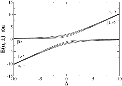
Figure 1: The energy non-linear dependence of the spectrum $E(n,\pm)-n\omega$ as a function of the detuning $\Delta$ for $\beta=1$. The non-linearity effects are stronger for low values of $n$.

III Jaynes-Cummings-Hubbard model

Optical cavities, with trapped atoms, can be arranged in arrays where the overlap between different cavities wave-functions allow photons to hop from one site to another. The Hamiltonian describing this new physical scenario is now known as Jaynes-Cummings-Hubbard model. The inclusion of optical fibres, or other optical devices, can be used to realize more complex geometries, where the hopping is not restricted to nearest neighbour cavities on a regular lattice Ritter ; Zheng ; Kyoseva . This is precisely the kind of situation that we want to investigate in this paper.

To tune the number of polaritons in each cavity a chemical potential $\mu$ might be used, hence the full JCH model will be described by the following Hamiltonian,

$$H^{JCH}=\sum_{i}\left[H_{i}^{JC}-\mu N_{i}\right]+H^{hop}$$ (6)

where

$$H^{JC}_{i}=\epsilon\sigma^{+}_{i}\sigma^{-}_{i}+\omega a^{{\dagger}}_{i}a_{i}+\beta(\sigma^{+}_{i}a_{i}+\sigma^{-}_{i}a^{{\dagger}}_{i})$$ (7)

is the Jaynes-Cummings Hamiltonian for a single cavity, and $N_{i}$ indicates the number of polaritons in each cavity ($N_{i}=\sigma^{+}_{i}\sigma^{-}_{i}+a^{{\dagger}}_{i}a_{i}$); while $H^{hop}$ is the hopping term. Note that the chemical potential $\mu$ is not an experimentally tunable parameter for this system. In real experiments appropriate preparation schemes have to be devised in order to obtain states with different polariton number. Recently, using the Rabi model, it has been shown that the inclusion of counter rotating terms can stabilize finite-density quantum phases of correlated photons without the use of a chemical potential Schiro . The last hopping term in Eq. (6) is characterized by a the strength $\kappa$ and the adjacency matrix of the underlying quantum network ${\tau}$, and is given by

$$H^{hop}=-\kappa\frac{1}{2}\sum_{i,j}\tau_{ij}(a^{{\dagger}}_{i}a_{j}+a^{{\dagger}}_{j}a_{i}).$$ (8)

Let us consider first two extreme cases: one in which the hopping strength is very small, and the other where the atom-photon interaction is negligible. In the atomic limit $\kappa/\beta\ll 1$, the Hamiltonian $H^{JCH}$ becomes, to first order approximation, the sum of single cavity Hamiltonians $H=\sum_{i}H_{i}$ , with $H_{i}$ given by

$$H_{i}=H_{i}^{JC}-\mu N_{i}.$$ (9)

The eigenstates of the single cavity Hamiltonian are given by Eqs. $(\ref{eigve})$ for $n\geq 1$ , and $\left|{0,\downarrow}\right\rangle=\left|{0}\right\rangle$ for $n=0$. The corresponding eigenvalues are

$$E_{n\pm}^{\mu}=(\omega-\mu)n+\frac{\Delta}{2}\pm\sqrt{n\beta^{2}+\frac{\Delta^{2}}{4}},$$ (10)

for $n\geq 1$, and $E_{0}=0$ for $n=0$. The ground state of the system can be calculated similarly to the case of a single cavity. Indeed, for every cavity we will found that the ground state is constituted either by the eigenstate $\left|{n,-}\right\rangle$ or by the eigenstate $\left|{0}\right\rangle$.

In the hopping dominated limit $\kappa/\beta\gg 1$ we can treat perturbatively the atom-photon interaction. $H^{JCH}$ reduces, to first-order approximation, to a tight-binding hamiltonian $H^{tb}$ given by

$$H^{tb}=\sum_{i}(\omega-\mu)a_{i}^{{\dagger}}a_{i}-\kappa\frac{1}{2}\sum_{i,j}\tau_{ij}(a^{{\dagger}}_{i}a_{j}+a^{{\dagger}}_{j}a_{i}){.}$$ (11)

The eigenvalues of $H^{tb}$ depends in a simple way from the eigenvalues $\lambda_{n}$ of the adjacency matrix of the quantum network:

$$E_{n}=N(\omega-\mu-\kappa\lambda_{n}).$$ (12)

The above equation reveals an instability of the system for

$$\kappa\Lambda>\omega-\mu$$ (13)

where $\Lambda$ is the maximal eigenvalue of the adjacency matrix ${\tau}$. From this result we can already conclude that the maximal eigenvalue of the adjacency matrix set an important scale for the strength of the hopping coefficient $\kappa$.

III.1 Mean-field theory

In order to explore the phase diagram of the Jaynes-Cummings-Hubbard model we make use of the mean-field treatment of the hopping term, which reduces to the following approximation

$$a_{i}a^{{\dagger}}_{j}\simeq\langle{a_{i}}\rangle a^{{\dagger}}_{j}+a_{i}\langle{a^{{\dagger}}_{j}}\rangle-\langle{a_{i}}\rangle\langle{a^{{\dagger}}_{j}}\rangle.$$ (14)

Therefore the hopping term becomes

$$H_{hop}^{MF}=-\kappa\sum_{i,j}\tau_{ij}(a^{{\dagger}}_{i}+a_{i})\psi_{j}+\kappa\sum_{i,j}\tau_{ij}\psi_{i}\psi_{j},$$ (15)

where we have indicated by $\psi_{i}$ the local order parameter $\psi_{i}\equiv\langle{a_{i}}\rangle$ (also equal to $\langle{a^{{\dagger}}_{i}}\rangle$, due to the gauge symmetry of the model). This Hamiltonian displays a phase transition between a Mott-Insulator phase, where $\psi_{i}=0$ $\forall i$, and a superfluid phase. In order to study the phase diagram of this model, within the mean-field approximation we treat $H^{hop}$ as a perturbation and we calculate $\psi_{i}$ self-consistently, to first order in $\kappa$, obtaining (see the Appendix for more details)

$$\psi_{i}=\kappa\sum_{j}\tau_{ij}\psi_{j}R_{n},$$ (16)

with $R_{n}$ given by

$$R_{0} = \left[\frac{\cos^{2}\theta_{1}}{E_{1-}^{\mu}}+\frac{\sin^{2}\theta_{1}}{E_{1+}^{\mu}}\right]$$ (17)

$$R_{n\geq 1} = -\left[\frac{|\sqrt{n+1}\cos\theta_{n}\cos\theta_{n+1}+\sqrt{n}\sin\theta_{n}\sin\theta_{n+1}|^{2}}{E^{\mu}_{n-}-E^{\mu}_{(n+1)-}}\right.$$

$$+ \frac{|\sqrt{n+1}\cos\theta_{n}\sin\theta_{n+1}-\sqrt{n}\sin\theta_{n}\cos\theta_{n+1}|^{2}}{E^{\mu}_{n-}-E^{\mu}_{(n+1)+}}$$

$$+ \frac{|\sqrt{n}\cos\theta_{n}\cos\theta_{n-1}+\sqrt{n-1}\sin\theta_{n}\sin\theta_{n-1}|^{2}}{E^{\mu}_{n-}-E^{\mu}_{(n-1)-}}$$

$$+ \left.\frac{|\sqrt{n}\cos\theta_{n}\sin\theta_{n-1}-\sqrt{n-1}\sin\theta_{n}\cos\theta_{n-1}|^{2}}{E^{\mu}_{n-}-E^{\mu}_{(n-1)+}}\right]$$

where the integer $n\geq 0$ depends on the systems parameters and it is chosen minimizing the on site energy $E_{n-}^{\mu}$given by Eq. (10). If we diagonalize Eq.$(\ref{psii})$, along with the eigenvalues of the adjacency matrix $\tau$, we get that the critical line for the transition between the Mott-insulator phase and the superfluid phase is given by

$$\kappa\Lambda R_{n}=1,$$ (18)

where $\Lambda$ is the maximal eigenvalue of the adjacency matrix $\tau$. This clearly shows that the phase diagram of the model depends on the product $\kappa\Lambda$. On regular graphs we have $\psi_{i}=\psi$ $\forall i$, and $\Lambda=z$, where $z$ is the connectivity of the lattice. On the other hand for complex topology the maximal eigenvalue of the hopping matrix $\Lambda$ can be significantly different from the average connectivity of the networks. In particular, for a large variety of networks the maximal eigenvalue of the adjacency matrix $\Lambda$ diverges with the network size. This suggests that, in order to have a non-trivial phase diagram for the Jaynes-Cummings-Hubbard model, the hopping strength $\kappa$ must scale as

$$\kappa\propto\frac{1}{\Lambda}.$$ (19)

In the following section we will investigate for different network topologies the respective scaling, with the network size, of the maximal eigenvalue of the adjacency matrix Chung ; K . We note here that at the mean-filed level the phase boundary is given by Eq.  $(\ref{crit})$. With respect to the phase diagram on regular lattices, the effect of the complex topology is the substitution of the average degree $z$ of the lattice with the maximal eigenvalue $\Lambda$ of the network. Therefore the dependence of the phase boundary on the detuning parameter $\Delta$ is similar to the one observed in regular lattices Pelster . In fact, as soon as the detuning is different from zero, the Mott lobes with mean polariton number greater than one are reduced in size and shifted to smaller value of the chemical potential. This effect is independent on the sign of the detuning parameter. We remark that on complex network as in regular lattices the thermal fluctuations destroy the Mott insulator phase. Therefore at finite temperature the phase diagram should be composed by a superfluid regime and a normal fluid.

$\begin{array}[]{c }{\includegraphics[width=173.44865pt]{figure2a.eps}}\\ {\includegraphics[width=173.44865pt]{figure2b.eps}}\\ {\includegraphics[width=173.44865pt]{figure2c.eps}}\\ \end{array}$

Figure 2: (Color online) Mean-field phase diagram of the Jaynes-Cummings-Hubbard model with $\Delta=0$ on a random scale-free network with power-law exponent $\gamma=2.2$ for different value of $N$, i.e. $N=100$ (top panel) $N=1000$ (middle panel) $N=10000$ (bottom panel). The phase diagram scales with the maximal eigenvalue that is given by $\Lambda=5.98$ (top panel) $\Lambda=11.07$ (middle panel) and by $\Lambda=23.42$ (bottom panel). The solid lines denote the analytic perturbative solution in mean field of the model.

III.2 Regular networks

For regular networks and regular lattices with connectivity $z$ the maximal eigenvalue of the adjacency matrix $\Lambda$ is independent on the network size. In particular, we have

$$\Lambda=z.$$ (20)

In this case the critical line Eq. $(\ref{crit})$ coincides with the one found in the literature using the mean-field approximation Greentree ; Greentree2 ; LeHur .

III.3 Random graphs

For random Erdös-Renyi graphs with finite connectivity and Poisson degree distribution, it has been proven K that

$$\Lambda\propto\sqrt{k_{max}},$$ (21)

where $k_{max}$ is the maximal degree of the system. For random networks with a finite connectivity we have $k_{max}=\ln N/\ln\ln N$, therefore

$$\Lambda(N)\propto\sqrt{\frac{\ln N}{\ln\ln N}}.$$ (22)

Considering the scaling given by Eq.$(\ref{scaling})$, we have that the hopping strength has to satisfy the following relation in order to have a non-trivial phase diagram

$$\kappa(N)\propto\sqrt{\frac{\ln\ln N}{\ln N}}.$$ (23)

III.4 Random scale-free networks

Scale-free networks provide one of the most interesting and most studied topology for the analysis of phase transitions occurring on them. Indeed, classically, on scale-free networks with degree distribution $P(k)\propto k^{-\gamma}$ and power-law exponent $\gamma\in(2,3]$ the phase diagram of the Ising model ising1 ; ising2 ; ising3 ; Bradde , and the percolation transition percolation1 ; percolation2 change drastically due to the diverging second moment of the average degree $\langle{k^{2}}\rangle$. A similar observation can be also made for the epidemic spreading model on annealed complex networks epidemics , i.e. complex networks in which the links are dynamically rewired. Moreover, the spectral properties of the complex networks determine the critical behavior of the epidemic spreading on complex quenched networks Durrett ; epidemics2 for the $O(N)$ model Burioni_ON1 ; Burioni_ON2 and the stability of the synchronization dynamics Synchr1 ; Synchr2 .

In random scale-free networks, with power-law degree distribution $P(k)\propto k^{-\gamma}$ it has been proven Chung that the maximal eigenvalue scales like

$$\Lambda\propto\left\{\begin{array}[]{ccc}\sqrt{k_{max}}&\mbox{for}&\gamma>2.5\\ \frac{\langle{k^{2}}\rangle}{\langle{k}\rangle}&\mbox{for}&\gamma<2.5.\end{array}\right.$$ (25)

Moreover, the maximal degree of the network satisfy $k_{max}=\min\left[{N^{1/2},N^{1/(\gamma-1)}}\right]$, where we have considered the structural cutoff of the degrees of the network for $\lambda\leq 3$. Therefore, the maximal eigenvalue of the network $\Lambda$ follow a different scaling with the network size, depending of the power-law exponent $\gamma$,

$$\Lambda(N)\propto\left\{\begin{array}[]{ccc}N^{1/[2(\gamma-1)]}&\mbox{for}&\gamma>3\\ N^{1/4}&\mbox{for}&2.5<\gamma\leq 3\\ N^{(3-\gamma)/2}&\mbox{for}&\gamma<2.5.\end{array}\right.$$ (27)

Finally, the hopping coefficient $\kappa$ that ensure a non-trivial phase diagram [see Eq. $(\ref{scaling})$] scales with the network size $N$ according to the following rules

$$\kappa(N)\propto\left\{\begin{array}[]{ccc}N^{-1/[2(\gamma-1)]}&\mbox{for}&\gamma>3\\ N^{-1/4}&\mbox{for}&2.5<\gamma\leq 3\\ N^{-(3-\gamma)/2}&\mbox{for}&\gamma<2.5\end{array}\right.$$ (29)

Figure2 shows both the analytic perturbative solution in mean-field of the JCH model, and the numerical non-perturbative mean-field evaluation of the phase diagram. As can be seen there is substantial agreement between the two, and furthermore one can observe the dependence on the size of the network of the detailed location of the critical lines.

$\begin{array}[]{c c}{\includegraphics[width=97.56383pt]{figure3a.eps}}&{\includegraphics[width=97.56383pt]{figure3b.eps}}\end{array}$

Figure 3: (Color online) Left panel: the first 3 generations of the Apollonian graph. The nodes and links added to construct the 1st, 2nd and 3rd generations are shown. Right panel: the 5th generation Apollonian network.

III.5 Apollonian networks

We consider here Apollonian networks Apollonian1 which are constructed through a 2D Apollonian packing model in which the space between three tangent circles placed on the vertices of an equilateral triangle is filled by a maximal circle. The space-filling procedure is repeated for every space bounded by three of the previously drawn tangent circles. The corresponding Apollonian network is constructed by connecting the centers of all the touching circles [Figure 3 (left)]. The resulting network is scale-free with power-law degree distribution $p(k)={\cal N}k^{-\lambda}$ and $\lambda=1+\ln(3)/\ln(2)\simeq 2.585$. Also these networks are known to have diverging maximal eigenvalue $\Lambda$ of their adjacency matrix Apollonian2 . In Figure 4 we plot the maximal eigenvalue $\Lambda$ of the apollonian network as a function of the network size $N$. We can fit the numerical results with the function

$$\Lambda(N)\propto N^{0.23}.$$ (30)

Therefore the hopping coefficient $\kappa$ [that needs to scale according Eq. (19)] scales for large $N$ as

$$\kappa(N)\propto N^{-0.23}.$$ (31)

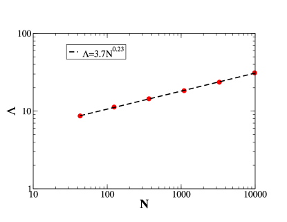
Figure 4: Scaling of the maximal eigenvalue $\Lambda$ of the Apollonian network as a function of the size $N$ of the network.

III.6 Small-world networks

Small-world networks structures characterize a system that has at the same time a small diameter, like random networks, but also has a high clustering coefficient, similarly to regular networks SW . In particular, we can follow the construction proposed in SW : we start from a regular chain in which each node is linked to the nearest neighbours and to the next-nearest neighbours; then every link is rewired with probability $p$ to another random node of the network. For $p=0$ the small-world network is a regular lattice in one dimension; for $p=1$ the small-world network becomes one instance of a random graph network; finally, for every intermediate value of $p$ we observe the small-world network with small average diameter and a high clustering coefficient. The maximal eigenvalue of this network, for $p=1$ will increases with $N$, as in the random graph case [Eq.(22)], while for the case $p=0$ it will be independent on $N$, as in regular networks. In Figure 5 we see how the maximal eigenvalue of the network changes with $N$ for intermediate values of the probability $p$ when the network is small-world.

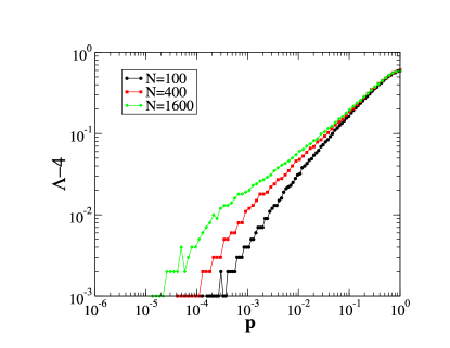
Figure 5: The maximal eigenvalue of the Small-World network as a function of $p$ for different network sizes $N$. In the limit $p\to 0$ the small world model is a regular chain with average connectivity $z=4$, therefore in this limit $\Lambda=4$. The data are averaged over 100 network realizations.

IV Conclusions

In conclusion we have studied the Jaynes-Cummings-Hubbard (JCH) model on complex quantum networks. We have shown that the phase diagram derived in the mean-field approximation, depends crucially on the maximal eigenvalue $\Lambda$ of the hopping matrix. In particular the phase diagram depends on the product $\kappa\Lambda$. This implies that in order to have a well defined phase diagram in the large network limit, the hopping coefficient $\kappa$ should scales proportionally to $1/\Lambda$. The eigenvalue $\Lambda$ is equal to the connectivity of the network, for regular networks and lattices, but for complex random networks it generally increases with the network size. In this paper we have listed for a large class of networks the scaling of the maximal eigenvalue $\Lambda$ with the network size $N$. For complex networks that have a diverging $\Lambda$, the hopping coefficient should be a decreasing function of $N$ in order to observe the phase transition from the Mott-like regime to the superfluid phase. This result implies the possibility of observing quantum critical behaviours in arrays whose cavities are weakly coupled, assuming the effective realization of the proper complex quantum network topology.

Appendix A Mean field solution of the JCH model

The Jaynes-Cummings Hamiltonian (we set $\hbar=1$)

$$H^{JC}=\epsilon\sigma^{+}\sigma^{-}+\omega a^{\dagger}a+\beta(\sigma^{+}a+\sigma^{-}a^{\dagger})$$ (32)

is obtained in the rotating wave approximation and in the limit $\beta\ll\epsilon,\omega$. The total number of excitations is a conserved quantity, and it is given by the sum of electromagnetic and atomic excitations $N=a^{\dagger}a+\sigma^{+}\sigma^{-}$. The interacting part of the Hamiltonian connects $n$-sectors which differs only by one photon excitation

$$\left|{n-1}\right\rangle\left|{\uparrow}\right\rangle\longleftrightarrow\left|{n}\right\rangle\left|{\downarrow}\right\rangle$$ (33)

The JC Hamiltonian can then be block-diagonalized in different sectors, each labelled by $n$, and each sector spanned by $\{\left|{n-1}\right\rangle\left|{\uparrow}\right\rangle,\left|{n}\right\rangle\left|{\downarrow}\right\rangle\}$. Choosing this set as the basis for the $n-$th sector, Eq.(2) and Eq.(4) in the main text provide the expressions for the eigenvectors and eigenvalues of the JC Hamiltonian.

Considering the situation of a network of cavities, whose coupling is effectively described by an hopping term, we have the Jaynes-Cummings-Hubbard Hamiltonian described in Eq.(6). As explained in the main text, the mean-field treatment of the hopping term allows us to approximate the JCH Hamiltonian as follows

$$H^{MF} = \sum_{i}\epsilon\sigma_{i}^{+}\sigma_{i}^{-}+\omega a_{i}^{\dagger}a_{i}+\beta(\sigma_{i}^{+}a_{i}+\sigma_{i}^{-}a_{i}^{\dagger})$$

$$-\kappa\sum_{i,j}\tau_{ij}(a^{{\dagger}}_{i}+a_{i})\psi_{j}+\kappa\sum_{i,j}\tau_{ij}\psi_{i}\psi_{j}.$$

Considering the hopping term as a perturbation to the atomic limit, the order parameter of the model is provided by $\psi_{i}\equiv\langle a_{i}\rangle_{gs}$, where the expectation value is calculated with respect to the ground-state of the Jaynes-Cummings-Hubbard model to first order in perturbation theory. Note that the order parameter can be assumed real due to the gauge symmetries of the Hamiltonian LeHur . The self-consistent equation for the order parameter can then be written as

$$\psi_{i}\equiv\langle n_{1}|a_{i}|n_{1}\rangle,$$ (34)

where $|n_{1}\rangle\equiv|n,-\rangle^{0}+|n\rangle^{1}$ is the approximation of the ground-state to first-order in the perturbation, while $|n,-\rangle^{0}$ is the ground-state of the unperturbed Hamiltonian (see Eq.2 in the main text), and

$$|n\rangle^{1}=\sum_{k,\alpha=\pm}\frac{{}^{0}\langle k,\alpha|H^{MF}_{hop}|n,-\rangle^{0}}{E^{\mu}_{n,-}-E^{\mu}_{k,\alpha}}|k,\alpha\rangle^{0}.$$

From Eq. (34) we have

$$\langle n_{1}|a_{i}|n_{1}\rangle = {}^{0}\langle n,-|a_{i}|n,-\rangle^{0}+\,^{1}\langle n|a_{i}|n\rangle^{1}$$

$$+\,^{0}\langle n,-|a_{i}|n\rangle^{1}+\,^{1}\langle n|a_{i}|n,-\rangle^{0}.$$

Keeping only non-zero terms to first order in $\kappa$ we are left only with the last two terms in the above equation. First we explicitly calculate

$${}^{0}\langle n,-|a_{i}|n\rangle^{1}=\sum_{k,\alpha=\pm}\frac{{}^{0}\langle k,\alpha|H^{MF}_{hop}|n,-\rangle^{0}}{E^{\mu}_{n,-}-E^{\mu}_{k,\alpha}}\,^{0}\langle n,-|a_{i}|k,\alpha\rangle^{0}.$$

It is easy to check that the only non-zero terms in the sum are given by $k=(n+1)$, and $\alpha=+,-$. It follows that the non-zero contribution to the expectation value of $H^{MF}_{hop}$ is provided only by $-\kappa\sum_{j}\tau_{ij}\hat{a}_{i}^{\dagger}\psi_{j}$. From the explicit form for the ground-states of the unperturbed Hamiltonian (see Eq.2 in the main text) we obtain

$${}^{0}\langle n,-|a_{i}|(n+1),-\rangle^{0} = \sqrt{n+1}\cos{\theta_{n}}\cos{\theta_{n+1}}$$

$$+\sqrt{n}\sin{\theta_{n}}\sin{\theta_{n+1}}$$

$${}^{0}\langle n,-|a_{i}|(n+1),+\rangle^{0} = \sqrt{n+1}\cos{\theta_{n}}\sin{\theta_{n+1}}$$

$$-\sqrt{n}\sin{\theta_{n}}\cos{\theta_{n+1}}.$$

We can proceed similarly for the calculation of ${}^{1}\langle n|a_{i}|n,-\rangle^{0}$, obtaining

$${}^{0}\langle(n-1),-|a_{i}|n,-\rangle^{0} = \sqrt{n}\cos{\theta_{n}}\cos{\theta_{n-1}}$$

$$+\sqrt{n-1}\sin{\theta_{n}}\sin{\theta_{n-1}}$$

$${}^{0}\langle(n-1),+|a_{i}|n,-\rangle^{0} = \sqrt{n}\cos{\theta_{n}}\sin{\theta_{n-1}}$$

$$-\sqrt{n-1}\sin{\theta_{n}}\cos{\theta_{n-1}}.$$

Now let us define

$$R_{n} \equiv -\sum_{\alpha=\pm}\left[\frac{|^{0}\langle n,-|a_{i}|(n+1),\alpha\rangle^{0}|^{2}}{E^{\mu}_{n,-}-E^{\mu}_{(n+1),\alpha}}\right.$$

$$+\left.\frac{|^{0}\langle(n-1),\alpha|a_{i}|n,-\rangle^{0}|^{2}}{E^{\mu}_{n,-}-E^{\mu}_{n-1,\alpha}}\right].$$

Putting everything together we have the following self-consistent equation to first order in perturbation theory (for $n>0$)

$$\psi_{i}=\kappa R_{n}\sum_{j}\tau_{ij}\psi_{j},$$

The case $n=0$ can be calculated in the same way and one has

$$\psi_{i}=\kappa R_{0}\sum_{j}\tau_{ij}\psi_{j},$$

where

$$R_{0}=-\sum_{\alpha=\pm}\frac{|\langle 0,\downarrow|a_{i}|1,\alpha\rangle|^{2}}{E^{\mu}_{0,\downarrow}-E^{\mu}_{1,\alpha}},$$

with $\langle 0,\downarrow|a_{i}|1,-\rangle=\cos{\theta_{1}}$, and $\langle 0,\downarrow|a_{i}|1,+\rangle=\sin{\theta_{1}}.$

References

- (1) M. J. Hartmann, F.G.S.L. Brandão and M.B. Plenio, Laser & Photonics Reviews 2, 527, (2008).
- (2) M. J. Hartmann, F.G.S.L. Brandão and M.B. Plenio, Nature Physics 2, 849 (2006).
- (3) H. J. Kimble, Nature 453, 1023 (2008).
- (4) S. Ritter, C. Nölleke, C. Hahn, A. Reiserer, A. Neuzner, M. Uphoff, M. Mücke, E. Figueroa, J. Bochmann G. Rempe, Nature 484, 195 (2012).
- (5) M. Schiró, M. Bordyuh, B. Öztop, and H. E. Türeci, Phys. Rev. Lett. 109, 053601 (2012).
- (6) E. T. Jaynes and F. W. Cummings, Proc. IEEE 51,89 (1963).
- (7) A. D. Greentree, C. Tahan, J. H. Cole L. C. L. Hollenberg Nature Physics 2, 856 (2006).
- (8) A. D. Greentree and L. C. L. Hollenberg in (Understanding Quantum Phase Transitions ) (Taylor & Francis, Boca Raton, 2011).
- (9) J. Koch K. Le Hur, Phys. Rev. A 80, 023811 (2009).
- (10) A. Faraon,A. Majumdar, and J. Vučković Phys. Rev. A 81, 033838 (2010).
- (11) S. Schmidt and G. Blatter, Phys. Rev. Lett. 104, 216402 (2010).
- (12) C. Nietner and A. Pelster, Phys. Rev. A 85,043831 (2012)
- (13) S. Sachdev Quantum Phase Transitions (Cambridge University Press,Cambridge,2000).
- (14) A. A. Houck, H. E. Türeci and J. Koch, Nature Physics 8, 292 (2012).
- (15) S.-B. Zheng,Applied Physics Letters,94, 154101 (2009).
- (16) E. Kyoseva, A. Beige and L. Chuan Kwek, New Journal of Physics, 14 023023 (2012).
- (17) S. Garnerone, P. Zanardi, D. A. Lidar, Phys. Rev. Lett. 108,230506 (2012).
- (18) S. Garnerone, Phys. Rev. A 86 032342 (2012).
- (19) E. Sánchez-Burillo, J. Duch, J. Gómez-Gardeñes, David Zueco, Scientific Reports 2, 605 (2012).
- (20) A. Cardillo, F. Galve, D. Zueco, J. Gómez-Gardeñes, arxiv:1211.2580
- (21) Burioni R., Cassi D., Rasetti M., Sodano P. Vezzani A. Jour. of Phys. B 34 4697 (2001).
- (22) M. Sade, T. Kalisky, S. Havlin and R. Berkovits Phys. Rev. E 72,066123 (2005).
- (23) L. Jahnke, J. W. Kantelhardt, R. Berkovits, S. Havlin Phys. Rev. Lett.101, 175702 (2010).
- (24) Andre M. C. Souza and H. Hermann Phys. Rev. B 75 054412 (2007).
- (25) I. N. de Oliveira, F.A. B. F. de Moura, M. L. Lyra, J.S. Andrade, Jr. and E.L. Albuquerque Phys. Rev. E 79 016104 (2009).
- (26) I. N. de Olivera, F. A. B. F. de Moura, M. L. Lyra Jr. and J. S. Albuquerque Phys. Rev. E 81 030104(R) (2010).
- (27) G. Bianconi Phys. Rev. E 85, 061113 (2012).
- (28) G. Bianconi, J. Stat. Mech. P07021 (2012).
- (29) A. Halu, L. Ferretti, A. Vezzani and G. Bianconi, EPL 99 18001 (2012).
- (30) K. Anand, G. Bianconi, S. Severini, Phys. Rev. E 83, 036109 (2011).
- (31) S. Garnerone, P. Giorda, P. Zanardi, New J. Phys. 14, 013011 (2012).
- (32) S. N. Dorogovtsev, A. Goltsev and J. F. F. Mendes, Rev. Mod. Phys. 80, 1275 (2008);
- (33) A. Barrat, M. Barthélemy, A. Vespignani Dynamical Processes on complex Networks (Cambridge University Press, Cambridge, 2008).
- (34) M. Fisher, P. Weichman, G. Grinstein D.S. Fisher, Phys. Rev. B 40 546 (1986).
- (35) M. Greiner, I. Bloch, O. Mandel, T. W. Hansch T. Esslinger, Phys. Rev. Lett.87, 160405 (2001).
- (36) L. Fallani, J. E. Lye, V. Guarrera, C. Fort M. Inguscio, Phys. Rev. Lett. 98, 130404 (2007).
- (37) P. Buonsante A. Vezzani, Phys. Rev. A 70, 033608 (2004).
- (38) P. Buonsante, F. Massel, V. Penna, A. Vezzani, Laser Physics17, 538 (2007).
- (39) J. S. Jr. Andrade, H. J. Herrmann, R. F. S. Andrade L. R. Silva, Phys. Rev. Lett. 94, 018702 (2005).
- (40) R. F. S. Andrade J. G. V. Miranda, Physica A 356, 1 (2005).
- (41) A. Imamoglu, H. Schmidt, G. Woods, and M. Deutsch, Phys. Rev. Lett. 79 1467 (1997).
- (42) K. M. Birnbaum, A. Boca, R. Miller, A. D. Boozer, T. E. Northup and H. J. Kimble, Nature 436 87 (2005).
- (43) D. G. Angelakis, M. Franca Santos, and S. Bose, Phys. Rev. A 76 031805 (2007).
- (44) F. Chung, L. Lu and V. Vu PNAS 100,6313 (2003).
- (45) M. Krivelevich and B. Sudakov Combinatorics, Probab. Comput. 12, 61 (2003).
- (46) G. Bianconi, Physics Letters A303,166(2002)
- (47) S. N. Dorogovtsev, A. V. Goltsev J. F. F. Mendes, Phys. Rev. E66,016104(2002).
- (48) M. Leone, A. Vázquez, A. Vespignani R. Zecchina, Eur. Phys. J. B 28, 191(2002).
- (49) S. Bradde, F. Caccioli, L. Dall’Asta G. Bianconi, Phys. Rev. Lett. 104 218701(2010).
- (50) R. Cohen, K. Erez, D. Ben-Avraham S. Havlin, Phys. Rev. Lett. 85,4626 (2000).
- (51) R. Cohen, K. Erez, D. Ben-Avraham S. Havlin, Phys. Rev. Lett. 86,3682(2001).
- (52) R. Pastor-Satorras A. Vespignani, Phys. Rev. Lett. 86,3200(2001).
- (53) R. Durrett PNAS 107,4491 (2010).
- (54) M. A. Muñoz, R. Juhász, C. Castellano, G. Ódor Phys. Rev. Lett. 105128701 (2010).
- (55) D. Cassi, Phys. Rev. Lett.76 2941(1996).
- (56) R. Burioni, D. Cassi A. Vezzani, Phys. Rev. E 60, 1500(1999).
- (57) M. Barahona L. M. Pecora Phys. Rev. Lett. 89,054101(2002).
- (58) T. Nishikawa, A. E. Motter, Y.-C. Lai, F. C. Hoppensteadt, Phys. Rev. Lett. 91, 014101 (2003).
- (59) D. J. Watts, S. H. Strogatz, Nature 393 409 (1998).