Compton Dominance and the Blazar Sequence

Abstract

Does the “blazar sequence” exist, or is it a result of a selection effect, due to the difficulty in measuring the redshifts of blazars with both high synchrotron peak frequencies ($\gtrsim 10^{15}\ \mathrm{Hz}$) and luminosities ($\gtrsim 10^{46}\ \mathrm{erg}\ \mathrm{s}^{-1}$)? We explore this question with a sample of blazars from the Second Catalog of Active Galactic Nuclei (AGN) from the Fermi Large Area Telescope (LAT). The Compton dominance, the ratio of the peak of the Compton to the synchrotron peak luminosities, is essentially a redshift-independent quantity, and thus crucial to answering this question. We find that a correlation exists between Compton dominance and the peak frequency of the synchrotron component for all blazars in the sample, including ones with unknown redshift. We then construct a simple model to explain the blazar properties in our sample, where the difference between sources is due to only the magnetic field of the blazar jet emitting region, the external radiation field energy density, and the jet angle to the line of sight, with the magnetic field strength and external energy density being correlated. This model can reproduce the trends of the blazars in the sample, and predicts blazars may be discovered in the future with high synchrotron peak frequencies and luminosities. At the same time the simple model reproduces the lack of high-synchrotron peaked blazars with high Compton dominances ($\gtrsim 1$).

1. Introduction

AGN with relativistic jets pointed along our line of sight are known collectively as blazars (e.g., Urry & Padovani, 1995). Blazars have two main sub-classes, those with strong broad emission lines, Flat Spectrum Radio Quasars (FSRQs), and those with weak or absent lines, known as BL Lacertae objects (BL Lacs; Marcha et al., 1996; Landt et al., 2004). FSRQs are thought to be Fanaroff-Riley (FR; Fanaroff & Riley, 1974) type II radio galaxies aligned along our line of sight, while BL Lac objects are thought to be aligned FR type I radio galaxies. In general, the spectral energy distributions (SEDs) of blazars have two basic components: a low frequency component, peaking in the optical through X-rays, from synchrotron emission; and a high frequency component, peaking in the $\gamma$ rays, probably originating from Compton scattering of some seed photon source, either internal (synchrotron self-Compton or SSC) or external to the jet (external Compton or EC).

Aside from their classifications as FSRQs or BL Lacs from optical spectra, Abdo et al. (2010c) subdivided them based on their synchrotron peak. They are considered high synchrotron-peaked (HSP) blazars if their synchrotron peak $\nu^{sy}_{pk}>10^{15}\ \mathrm{Hz}$; intermediate synchrotron-peaked (ISP) blazars if $10^{14}\ \mathrm{Hz}<\nu^{sy}_{pk}<10^{15}\ \mathrm{Hz}$; and low synchrotron-peaked (LSP) blazars if $\nu^{sy}_{pk}<10^{14}\ \mathrm{Hz}$. Almost all FSRQs are LSP blazars.

Fossati et al. (1998) combined several blazar surveys and noted an anti-correlation between the luminosity at the synchrotron peak, $L_{pk}^{sy}$, and the frequency of this peak, $\nu^{sy}_{pk}$. They also noticed anti-correlations between the 5 GHz luminosity ($L_{5\ GHz}$) and $\nu^{sy}_{pk}$; the $\gamma$-ray luminosity and $\nu^{sy}_{pk}$; and the $\gamma$-ray dominance (the ratio of the EGRET $\gamma$-ray luminosity to the synchrotron peak luminosity) and $\nu^{sy}_{pk}$. These correlations were claimed as evidence for a “blazar sequence”, a systematic trend from luminous, low-peaked, $\gamma$-ray dominant sources with strong broad emission lines to less luminous, high-peaked sources with weak or nonexistent broad emission lines and $\gamma$-ray dominance $\sim 1$. Ghisellini et al. (1998) provided a physical explanation for these correlations. If the seed photon source for external Compton scattering is the broad-line region (BLR), and the BLR strength is correlated with the power injected into electrons in the jet, one would expect that more luminous jets have stronger broad emission lines and greater Compton cooling, and thus a lower $\nu^{sy}_{pk}$. As the power injected in electrons is reduced, the broad line luminosity decreases, there are fewer seed photons for Compton scattering, and consequently the peak synchrotron frequency moves to higher frequencies. This trend is also reflected in the lower luminosity of the Compton-scattered component relative to the synchrotron component as $\nu^{sy}_{pk}$ moves to higher frequencies. If this physical explanation is correct, it provides a powerful tool for understanding blazars and their evolution, not unlike the “main sequence” for stars on the Hertzsprung- Russel diagram. The blazar sequence also has implications for “feedback”, a relationship where the AGN jet heats the hot, X-ray emitting intracluster medium (ICM), while the ICM gas Bondi accretes onto the black hole, providing the fuel for the jet (e.g., Bîrzan et al., 2004). Hardcastle et al. (2007) have suggested that radio galaxies without high excitation narrow lines (mostly FR Is, and presumably BL Lacs) are fed by “hot mode” accretion, i.e., accretion from the hot ICM; while radio galaxies with high excitation narrow lines (mostly FR IIs, and presumably FSRQs) are fed by “cold mode” accretion, i.e., accretion of cold gas unrelated to the ICM.

The $L_{pk}^{sy}$–$\nu_{pk}^{sy}$ anti-correlation has been questioned. Using blazars from the Deep X-ray Radio Blazar Survey and the ROSAT All-Sky Survey/Green Bank Survey, Padovani et al. (2003) did not find any anti-correlation between $\nu^{sy}_{pk}$ and radio, BLR, or jet power. This work, however, has been criticized for its relatively poor SED characterization (Ghisellini & Tavecchio, 2008b). Padovani (2007) has identified several major predictions of the blazar sequence: the anti-correlation will continue to be found in more complete samples; since low luminosity objects are almost always more plentiful than high luminosity objects, high-peaked blazars should be more plentiful than low-peaked blazars; and the lack of plentiful outliers, i.e., objects that are low-peaked and faint, or high-peaked and bright. If any of these predictions are contradicted, it would invalidate the sequence.

Ghisellini & Tavecchio (2008b) pointed out that since blazars are anisotropic emitters, the lower left of the diagram (i.e., sources that have low peaked, faint synchrotron components) should be filled in by sources which are viewed increasingly off-axis. But the lack of sources in the upper right region of the $L_{pk}^{sy}$–$\nu_{pk}^{sy}$ plot (i.e., sources that have high-peaked, bright synchrotron components) could be the result of a selection effect (Giommi et al., 2002; Padovani et al., 2002; Giommi et al., 2005, 2012a). Since a large fraction of BL Lac objects have entirely featureless optical spectra, their redshifts, $z$, and hence luminosities, are impossible to determine. These could be extremely luminous, distant BL Lacs that would fill in the upper right region. Nieppola et al. (2006) found no correlation between the frequency and luminosity of the synchrotron peaks for objects in the Metsähovi Radio Observatory BL Lacertae sample. Chen & Bai (2011) did find an anti-correlation, using sources found in the LAT bright AGN sample (Abdo et al., 2009a, 2010c). In recent works, an “L”-shape in the $L_{pk}^{sy}$–$\nu_{pk}^{sy}$ plot seems to have emerged, as lower luminosity low-peaked sources have been detected with more sensitive instruments (Meyer et al., 2011; Giommi et al., 2012b). Nieppola et al. (2006) found more of a “V” shape, although their plot did not include FSRQs; if high luminosity and low-peaked FSRQs were added, it might appear as more of an “L”. None of the studies that find few sources with high $L_{pk}^{sy}$ and high $\nu_{pk}^{sy}$ have yet to address the sources without redshifts, however. Rau et al. (2012) provide reliable photometric redshifts for 8 BL Lacs at $z\gtrsim 1.3$, and four of these do indeed seem to have $\nu_{pk}^{sy}\gtrsim 10^{15}$ Hz and $L_{pk}^{sy}\gtrsim 10^{46}\ \mathrm{erg}\ \mathrm{s}^{-1}$ (Padovani et al., 2012).

With the advent of the Fermi Gamma-Ray Space Telescope era, it is now possible to also characterize the Compton peak frequency $\nu_{pk}^{C}$ and luminosity $L_{pk}^{C}$ for a larger number of objects than previously possible with EGRET. As we show, the Compton dominance $A_{C}\equiv L_{pk}^{C}/L_{pk}^{sy}$ is an important parameter for characterizing this sequence, since it is a redshift-independent quantity. We explore the sequence using a sample based on the second catalog of AGN from the LAT (2LAC; Ackermann et al., 2011) in Section 2. We then show in Section 3 that the sequence, including sources with high $L_{pk}^{sy}$ and high $\nu_{pk}^{sy}$ can be reproduced with a simple model involving power-law injection of electrons and radiative cooling. Finally, we conclude with a discussion of these results (Section 4).

2. The 2LAC Blazar Sequence

2.1. Sample Definition and SED Characterization

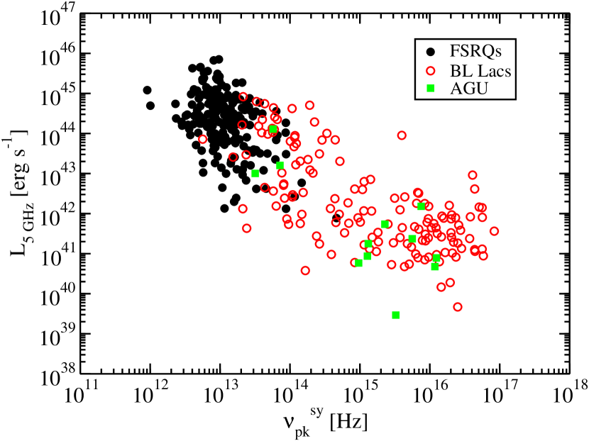
The 2LAC (Ackermann et al., 2011) presents the largest $\gamma$-ray catalog of blazars yet. It allows for the characterization of the high energy component for a greater number of blazars than previously possible. Here we look at the blazar sequence among the 2LAC clean sample, which includes 886 total sources, with 395 BL Lacs, 310 FSRQs, and 157 sources of unknown type. Ackermann et al. (2011) collected the fluxes of many of these sources at 5 GHz, 5000 Å, and 1 keV, and used empirical relations for finding the peak frequency of the synchrotron component from the slope between the 5 GHz and 5000 Å flux ($\alpha_{ro}$), and between the 5000 Å and 1 keV flux ($\alpha_{ox}$) found by Abdo et al. (2010c). Abdo et al. (2010c) in turn had found these empirical relations by fitting the broadband SEDs of 48 of the blazars in the 3-month LAT bright AGN sample (LBAS; Abdo et al., 2009a) with third degree polynomials to determine the peak synchrotron frequency, $\nu_{pk}^{sy}$. With the $\nu_{pk}^{sy}$ estimated from the empirical relations, Ackermann et al. (2011) could classify the objects in the 2LAC sample as LSP, ISP, or HSP. Here we use their results for $\nu_{sy}^{pk}$, which are corrected for redshift, and so are in the sources’ rest frames. The 2LAC also includes the 5 GHz flux density for many sources. We combine this with a spectroscopic redshift measurement, if available, or photometric redshifts found by Rau et al. (2012), to get the luminosity distance, $d_{L}$ and calculate the 5 GHz luminosity $L_{5\ GHz}=4\pi d_{L}^{2}(\nu F_{\nu})_{5\ GHz}$. We have corrected the radio luminosities to how they would appear in the rest frames of the sources (i.e., $k$-corrected them), assuming $\alpha_{r}=0$, where the radio flux density is $F_{\nu}\propto\nu^{-\alpha_{r}}$. A plot of $L_{5\ GHz}$ versus $\nu_{pk}^{sy}$ for the objects in the 2LAC clean sample for which the catalog has a listed $\nu^{sy}_{pk}$, 5 GHz flux density, and $z$ (or a $z$ from Rau et al., 2012) is given in Figure 1. This includes 352 sources, of which 145 are BL Lacs, 195 are FSRQs, and 12 are AGN of unknown optical spectral type (AGUs; i.e., unknown whether they are FSRQs or BL Lacs).

Figure 1.— Radio luminosity at 5 GHz versus peak synchrotron frequency for the 2LAC clean sample. Symbols are the same as in Figure 2.

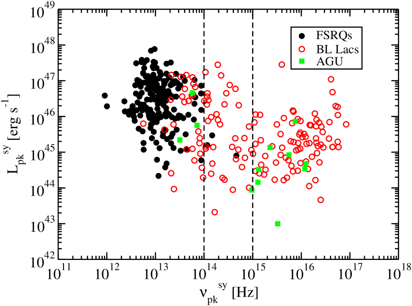
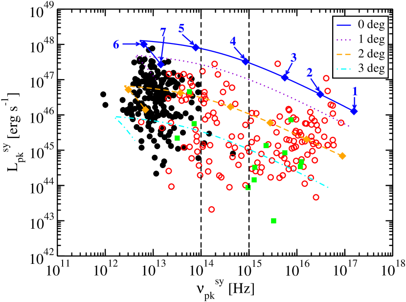
Abdo et al. (2010c) also provided an empirical formula for determining the flux at the synchrotron peak ($F_{pk}^{sy}$) from the the 5 GHz flux density and $\nu_{pk}^{sy}$. We use this empirical relation to determine the peak synchrotron flux for the 352 objects in our sample, and again combine it with $d_{L}$ to calculate the peak synchrotron luminosity, $L_{pk}^{sy}$. A resulting plot of $L_{pk}^{sy}$ versus $\nu_{pk}^{sy}$ is shown in Figure 2.

epsscale1.0

Figure 2.— Peak synchrotron luminosity versus peak synchrotron frequency for objects in the 2LAC clean sample. Filled circles represent FSRQs, empty circles represent BL Lacs, and filled squares represent objects which do not have an unambiguous classification. Dashed lines indicate the boundary between HSPs and ISPs ($\nu_{pk}^{sy}=10^{15}\ \mathrm{Hz}$) and between ISPs and LSPs ($\nu_{pk}^{sy}=10^{14}\ \mathrm{Hz}$).

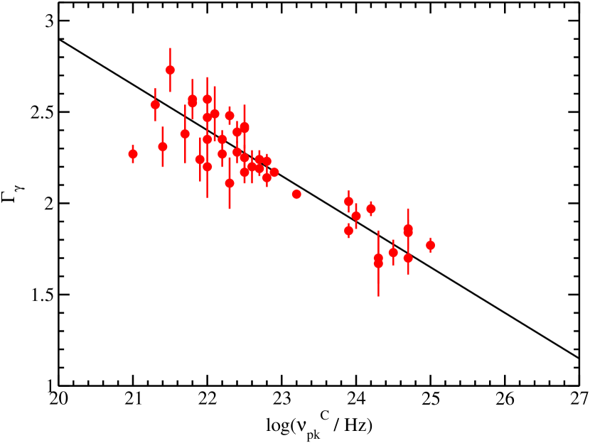
Additionally, Abdo et al. (2010c) fit the high energy components of their 48 LBAS blazars with a third degree polynomial to determine the peak of the $\gamma$-ray component (presumably from Compton scattering). They found an empirical relation between $\nu_{pk}^{C}$ and the LAT $\gamma$-ray spectral index, $\Gamma_{\gamma}$. Figure 3 shows $\Gamma_{\gamma}$ and $\nu_{pk}^{C}$ from their polynomial fits to the objects in their sample, and the empirical relation they found. The empirical fit seems reasonable in the range $1.6<\Gamma_{\gamma}<2.6$, but extending the relation outside this range is questionable. Approximately 10% of the 352 sources are also found in the 58-month Swift Burst Alert Telescope (BAT) catalog. For these sources, we extrapolated their BAT and LAT power-laws and found where the extrapolations intersected. If they intersected within the range 195 keV to 100 MeV (that is, in between the BAT and LAT bandpasses) we used this location as $\nu_{pk}^{C}$. Using the BAT spectrum in this way allows an improved estimation of $\nu_{pk}^{C}$ over the empirical relation from Abdo et al. (2010c), particularly for those very soft sources, for which this empirical relation is untested. For other sources, the peak was determined from the LAT spectral index and the empirical relation from Abdo et al. (2010c). In principle, a similar technique could be used by combining the LAT spectra and very-high energy (VHE) spectra taken from atmospheric Cherenkov telescopes, in order to find $\nu_{pk}^{C}$ for hard LAT sources. However, the VHE spectra tend to be highly variable, and are not integrated over a long period of time, and often are not simultaneous with the LAT spectra. Since the BAT and LAT spectra overlap in time and are integrated over long times, it seems more reasonable that they would represent a similar state.

Figure 3.— The LAT spectral index ($\Gamma_{\gamma}$) and the peak frequency of the Compton component, $\nu_{pk}^{C}$ determined from third-order polynomial fits from Abdo et al. (2010c), plotted as circles. The empirical fit they determined is plotted as the line.

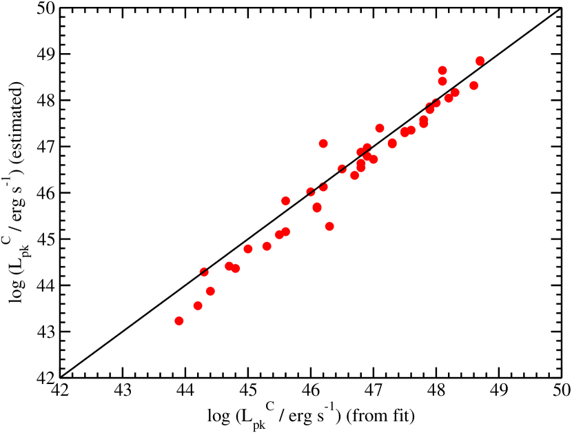
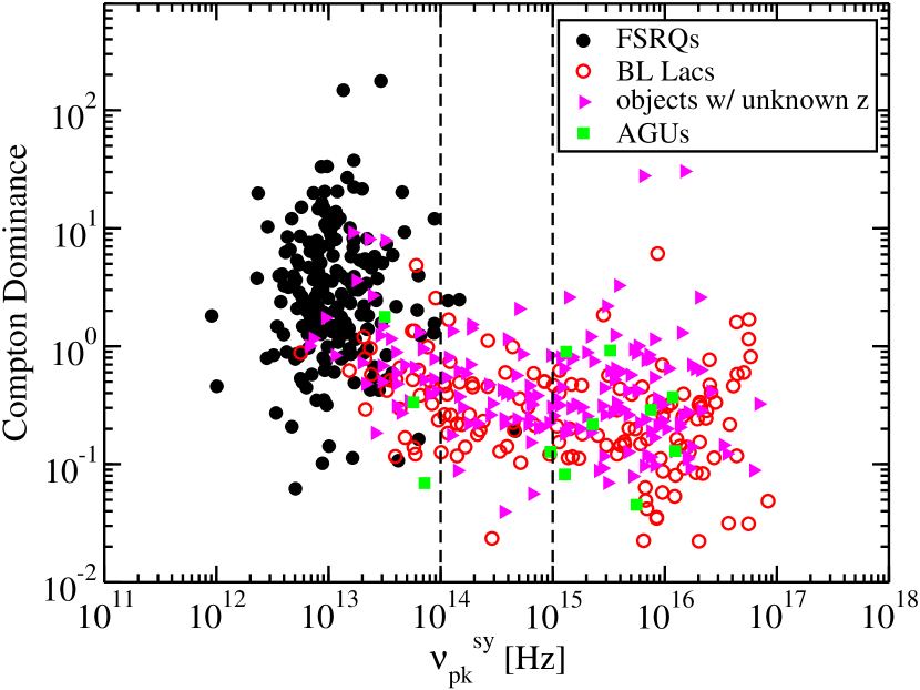
Once the location of $\nu_{pk}^{C}$ is known, either by using the empirical relation or from the BAT-LAT intersection, the flux at the peak, $F_{pk}^{C}$, can be estimated by extrapolating the LAT spectrum, and the corresponding luminosity can be calculated with $L_{pk}^{C}=4\pi d_{L}^{2}F_{pk}^{C}$. To test the accuracy of this approximation, we use this method to estimate $L_{pk}^{C}$ for the sample in Abdo et al. (2010c), and compare it with the value found by their fits to 48 sources. The results can be found in Figure 4; the agreement seems reasonable. Therefore, we used this technique to estimate $L_{pk}^{C}$ for the 352 objects in our sample. With this, we can calculate the Compton dominance, $A_{C}=L_{pk}^{C}/L_{pk}^{sy}$. A plot of $A_{C}$ versus $\nu_{pk}^{sy}$ is shown in Figure 5. Also note that $A_{C}$ is independent of redshift ($A_{C}=L_{pk}^{C}/L_{pk}^{sy}\approx F_{pk}^{C}/F_{pk}^{sy}$). Thus we can plot in Figure 5 an additional 170 sources from the 2LAC clean sample that have well-determined synchrotron bumps but do not have known redshifts. For these sources, the plotted $\nu_{pk}^{sy}$ is a lower limit, since the redshifts are not known. However, $\nu_{pk}^{sy}$ will be larger by only a factor $(1+z)$, i.e., a factor of a few.

Figure 4.— The peak Compton luminosity, $L_{pk}^{C}$, estimated from empirical relations as discussed in the text, plotted versus $L_{pk}^{C}$ determined from the fits by Abdo et al. (2010c). The line shows where the estimated and fit values would be equal.

Figure 5.— Compton dominance (i.e., $L_{pk}^{C}/L_{pk}^{sy}$) versus peak synchrotron frequency. Symbols are the same as in Figures 1 and 2; additionally, rightward-pointing triangles represent BL Lacs with unknown redshifts, for which $\nu_{pk}^{sy}$ is a lower limit.

2.2. Luminosity and the Sequence

In their diagrams of $L_{pk}^{sy}$ versus $\nu_{pk}^{sy}$, Nieppola et al. (2006) and Meyer et al. (2011) note a “V” or “L” shape. This shape is not at all obvious in our version of this plot in Figure 2. To determine the strength of the correlation between $L_{pk}^{sy}$ and $\nu_{pk}^{sy}$, we have computed the Spearman ($\rho$) and Kendall ($\tau$) rank correlation coefficients and the probability of no correlation (PNC) calculated from each coefficient. The results can be found in Table 1. The results from $\rho$ and $\tau$ are similar in all cases. The PNC is very small for the BL Lacs and FSRQs separately, and even lower for all the sources combined, where the probability is essentially zero that there is not a correlation. The small PNC is consistent with Fossati et al. (1998), who find essentially a zero chance of no correlation using the $\tau$ test. Note however that sources with unknown $z$ are not included. Since these sources could have high $L_{pk}^{sy}$, their exclusion could explain the anti-correlations for the whole sample and for the BL Lacs in general (Giommi et al., 2012a), since they could fill in the upper right part of this diagram, as mentioned in Section 1. Indeed, several sources with redshifts estimated from photometry have been found in this region (Padovani et al., 2012; Rau et al., 2012), and are included in our sample. The objects with unknown $z$ are almost certainly BL Lacs (i.e., they probably have small broad-line equivalent widths, making their redshifts difficult to determine), so it would not affect the hint (92.7% and 93.4% for the $\rho$ and $\tau$ coefficients, respectively) of anti-correlation found for FSRQs. It should also be noted that Nieppola et al. (2006) did not find a correlation between $L^{sy}_{pk}$ and $\nu^{sy}_{pk}$ for BL Lacs using the $\rho$ coefficient, possibly because they used log-parabola functions to characterize the SEDs, while Fossati et al. (1998) and Abdo et al. (2010c) use third-degree polynomials. Since our determinations of $\nu_{pk}^{sy}$ and $L_{pk}^{sy}$ are based on empirical relations related to these third-degree polynomial fits, our results could also be expected to be different from those of Nieppola et al. (2006).

Fossati et al. (1998) also found a significant anti-correlation between the 5 GHz luminosity, $L_{5\ GHz}$, and $\nu_{pk}^{sy}$, using the $\tau$ test. Like them, we find the anti-correlation with $L_{5\ GHz}$ versus $\nu_{pk}^{sy}$ (Figure 1) to be much more significant than the one between $L_{pk}^{sy}$ and $\nu_{pk}^{sy}$, as can be seen in Table 1. This is true for both FSRQs and BL Lacs alone as well as together. If the anti-correlation is explained by the increasing cooling at higher luminosities (Ghisellini et al., 1998), one might expect the correlation with $L^{sy}_{pk}$ to be more significant, since the emission at 5 GHz is thought to be from a different region of the jet than the emission at the peak, and the region emitting at the peak should be synchrotron self-absorbed at 5 GHz. However, since $\nu_{pk}^{sy}$ was determined in part based on the 5 GHz flux, the strong correlation with $L_{5\ GHz}$ is probably a result of this dependence. As pointed out by Lister et al. (2011), if $\nu_{pk}^{sy}$ increases, but its spectral shape and $\nu F_{\nu}$ peak flux do not change, the radio flux (or luminosity) will naturally decrease. This can easily explain this anti-correlation. However, what is unclear is whether a peak frequency derived from the radio flux should be interpreted as a cooling break, since these two should be from different regions and possibly independent. Determination of $\nu_{pk}^{sy}$ independent of low radio frequency emission should be a good, although technically challenging, way to test this.

Table 1Statistics of correlations involving $\nu_{pk}^{sy}$.

Sample	$\rho$	PNC($\rho$)	$\tau$	PNC($\tau$)
$L_{pk}^{sy}$ versus $\nu_{pk}^{sy}$
BL Lacs	-0.19	0.020	-0.12	0.035
FSRQs	-0.12	0.073	-0.088	0.066
All sources with known $z$	-0.54	$4.2\times 10^{-28}$	-0.35	$<10^{-50}$
$L_{5GHz}$ versus $\nu_{pk}^{sy}$
BL Lacs	-0.64	$5.4\times 10^{-18}$	-0.45	$<10^{-50}$
FSRQs	-0.36	$1.82\times 10^{-7}$	-0.25	$1.79\times 10^{-7}$
All sources with known $z$	-0.79	$<10^{-50}$	-0.58	$<10^{-50}$
$A_{C}$ versus $\nu_{pk}^{sy}$
BL Lacs	-0.30	$2.7\times 10^{-4}$	-0.21	$1.3\times 10^{-4}$
FSRQs	$8.9\times 10^{-3}$	0.90	$6.3\times 10^{-3}$	0.89
All sources with known $z$	-0.66	$9.8\times 10^{-45}$	-0.45	$<10^{-50}$
All sources 1	-0.66	$<10^{-50}$	-0.46	$<10^{-50}$
All sources 2	-0.66	$<10^{-50}$	-0.46	$<10^{-50}$
All sources 3	-0.64	$<10^{-50}$	-0.44	$<10^{-50}$

2.3. Compton Dominance and the Sequence

Combining their results with EGRET data, Fossati et al. (1998) made a plot of $\gamma$-ray dominance versus $\nu_{pk}^{sy}$. Using LAT data from the 2LAC, as described in Section 2.1, we make a similar plot (Figure 5), although we use $L_{pk}^{C}$ instead of simply the $\gamma$-ray luminosity. A distinct “L” shape is seen in this figure. We have also computed the correlation coefficients $\rho$ and $\tau$ for $A_{C}$ versus $\nu_{pk}^{sy}$, and the results can be found in Table 1. First we do this only for sources with known $z$. There is no evidence for a correlation for the FSRQs alone, although the probability that there is no correlation for the BL Lacs alone is very small. For the combined sample of all sources with known $z$, there is essentially zero chance that there is no correlation, similar to the $L_{pk}^{sy}$ versus $\nu_{pk}^{sy}$ correlation. Fossati et al. (1998) also find a low probability that there is no correlation using the $\tau$ test, although our result is stronger. We also computed the coefficients for all sources, including the ones with unknown $z$, computing their $\nu_{pk}^{sy}$ assuming $z=0$ (“all sources 1” in Table 1). We find essentially no chance that the addition of sources with unknown $z$ could ruin the correlation when these sources are included. The term $\nu_{pk}^{sy}$ will vary by a factor of a few due to redshift, so we also calculated the coefficients assuming all these sources with unknown $z$ are at $z=0.35$, the average of the BL Lacs with known $z$ (“all sources 2”); and assuming these sources are at $z=4$ (“all sources 3”), which is significantly higher than the maximum redshift of the entire sample (which is $z=3.1$). In each case, there is essentially a 100% chance that an anti-correlation exists. Although the correlation between $L_{pk}^{sy}$ and $\nu_{pk}^{sy}$ could exist only because of a redshift selection effect, a similar redshift selection effect cannot explain the correlation between $A_{C}$ and $\nu_{pk}^{sy}$. The relationship between $A_{C}$ and $\nu_{pk}^{sy}$ thus seems to have a physical origin.

Although a similar quantity, $\gamma$-ray dominance, was discussed as part of the original “blazar sequence” by Fossati et al. (1998), $\gamma$-ray dominance or Compton dominance has been mostly overlooked ever since, in favor of testing the correlation between $L_{pk}^{sy}$ and $\nu_{pk}^{sy}$ (e.g., Padovani et al., 2003; Nieppola et al., 2006; Padovani, 2007; Meyer et al., 2011; Giommi et al., 2012a), although see Giommi et al. (2012b) for a brief discussion. This neglect may be in part due to a lack of quality $\gamma$-ray data, a deficiency that has been corrected in the Fermi era.

2.4. Errors and Outliers

The errors on determining $\nu_{pk}^{sy}$ and $L_{pk}^{sy}$ have essentially been ignored in the past. Although for radio and optical observations measurement errors are small, clearly the peak will depend on how well-sampled the synchrotron bump is. Furthermore, X-ray measurements can have large errors (due in part to the necessity of assuming a spectral form to convolve with the response matrix of an X-ray instrument), and here ignoring their errors could lead to significant errors on $\nu_{pk}^{sy}$ and $L_{pk}^{sy}$. It is also possible that the peak location can depend on the fitting function used. It does not seem to be standardized; sometimes a log-parabola function is used (e.g., Nieppola et al., 2006), sometimes a third degree polynomial is used (e.g., Fossati et al., 1998; Abdo et al., 2010c; Meyer et al., 2011) and sometimes a physically-motivated synchrotron/Compton model is used (e.g., Padovani et al., 2003), although the third-order polynomial fit is the most common.

When locating the Compton peak, the measurement errors can have an even greater effect, since the $\gamma$-ray error bars tend to be larger than at lower frequencies. This can lead to significant errors in determining $A_{C}$. Abdo et al. (2010c) have estimated the error between the approximate expressions and the polynomial fits to be about an order of magnitude. This estimate still neglects the measurement errors, which can have a large effect on results.

The two sources with unknown redshifts in the upper right quadrant of Figure 5 are 2FGL J0059.2-0151 (1RXS 005916.3-015030) and 2FGL J0912.5+2758 (1RXS J091211.9+27595) with LAT spectral indices of $\Gamma_{\gamma}=1.15\pm 0.36$ and $\Gamma_{\gamma}=1.20\pm 0.37$, respectively. These are the two hardest sources in the 2LAC, and the sources with the largest error bars on their spectral indices; only one source in the 2LAC clean sample is fainter than these sources (2FGL J1023.6+2959). They are clearly outliers. Propagating the error on their spectral indices, one finds that they have Compton dominances of $\log_{10}(A_{C})=1.44\pm 1.82$ and $\log_{10}(A_{C})=1.48\pm 1.98$, respectively; they have $A_{C}$ consistent with unity within their error bars, and so are consistent with the “L” shape seen in Figure 5.

There are several FSRQ outliers in Figure 5 as well; perhaps most interesting are those with $A_{C}>10^{2}$. These three sources are: 2FGL J1017.0+3531 associated with B2 1015+35B; 2FGL J1154.4+6019 associated with CRATES J1154+6022; and the most extreme, 2FGL J1522.0+4348 associated with B3 1520+437, with $A_{C}=1500$, which is not shown in Figure 5. The sources 2FGL J1017.0+3531 and 2FGL J1522.0+4348 are estimated to have Compton components peaking in the BAT bandpass, both with peak fluxes $>6\times 10^{-10}\ \mathrm{erg}\ \mathrm{s}^{-1}\ \mathrm{cm}^{-2}$, and both would then be visible with BAT. The source 2FGL J1154.4+6019 is estimated to have a high-energy peak observed at 577 keV. Extrapolating from this peak back into the BAT bandpass with a spectral index $\Gamma=1.5$ gives a flux of $9.6\times 10^{-11}\ \mathrm{erg}\ \mathrm{s}^{-1}\ \mathrm{cm}^{-2}$ at 100 keV. There are several objects in the BAT catalog with fluxes less than this, so the BAT would probably have detected this source as well, if this estimate is correct. Thus, these three sources probably have a low-energy cutoff in their Compton component before the BAT waveband, and their $A_{C}$ shown here are probably not accurate.

Variability is another factor that can affect correlations determined here. Blazars are highly variable at all wavelengths, and the peaks of blazars can vary by several orders of magnitude (Fossati et al., 2000; Costamante et al., 2001). Giommi et al. (2012b) explore the issue of characterizing peaks at different epochs from microwave, X-ray, and $\gamma$-ray data. They conclude that microwave variations are rather minimal and make little difference in characterizing SEDs, but variations in X-rays (0.1 - 2.4 keV) and $\gamma$-rays (in the LAT energy band) can vary by up to a factor of 10 or greater.

For all of these reasons, the results in Figures 1, 2, and 5 are probably not accurate for individual sources, although no one has rigorously estimated their errors. However, we are more interested in the overall trend than individual sources, so the trend could still be present even for large errors. To test if it will still be present, we performed a simple Monte Carlo simulation. For each source, we randomly drew the LAT spectral index ($\Gamma_{\gamma}$) and luminosity ($L_{\gamma}$) from the measured values and measurement errors, assuming the errors are described by normal distributions. Then we used this randomly-drawn value to calculate $A_{C}$. There are no reported errors on $\nu_{pk}^{sy}$, so we assumed that $\log(\nu_{pk}^{sy})$ has normally-distributed errors of one decade. We then used the Spearman and Kendall tests on the randomly-drawn distribution to determine if the correlation persists. We performed this simulation $10^{5}$ times, and found that a PNC $>5.7\times 10^{-7}$ (the probability corresponding to $5\sigma$, assuming normally distributed errors) was found in only around 5% of the simulations, for both $\rho$ and $\tau$ tests. Thus, we are confident that the trend persists despite large (random) errors. There do not seem to be any systematic errors in using the empirical relations instead of the polynomial fits (Abdo et al., 2010c, Figures 3 and 4), except possibly a small systematic underestimation of $L_{pk}^{C}$ as shown in Figure 4.

3. Theoretical Blazar Sequence

3.1. Simple Unified Blazar Emission Model

We describe a simple model for blazar jet emission, and show that it can reproduce blazar properties described in Section 2. This model is similar to the ones presented by Böttcher & Dermer (2002) and Ghisellini & Tavecchio (2008b); Ghisellini et al. (2009). We assume the relativistic jet is dominated by emission from a single zone which is spherical with radius $R^{{}^{\prime}}_{b}$ in its comoving frame, and moving with highly relativistic speed $\beta c$ giving it a Lorentz factor $\Gamma=(1-\beta^{2})^{-1/2}$. The jet makes an angle to the line of sight $\theta$ so that the Doppler factor $\delta_{\rm D}=[\Gamma(1-\beta\cos\theta)]^{-1}$. Electrons are injected with a power-law distribution given by

$$Q_{e}(\gamma)=Q_{0}\gamma^{-q}\ H(\gamma;\gamma_{1},\gamma_{2})\ ,$$ (1)

where the Heaviside function $H(x;a,b)=1$ for $a<x<b$ and $=0$ everywhere else. In terms of a blast wave model, high $\gamma_{1}$ can come about in highly energetic, fast shocks, where a high fraction of the swept up energy is used to accelerate particles, and the lower-energy part of the distribution becomes particle-starved (e.g., Dermer et al., 2000; Dermer & Menon, 2009). The hard X-ray spectra in some blazars may indicate very hard electron spectra at lower energies (Sikora et al., 2009). Although blazars can be quite variable on timescales as short as hours (e.g., Abdo et al., 2009b) or even minutes (Aharonian et al., 2007), we will assume their average or quiescent emission can be described by a steady state solution to the electron continuity equation, where continuous injection is balanced by cooling and escape. The power continuously injected in electrons is given by

$$L_{inj,e}=m_{e}c^{2}\int^{\gamma_{2}}_{\gamma_{1}}\ d\gamma\ \gamma\ Q_{e}(\gamma)\ ,$$ (2)

or, using Equation (1),

$$L_{inj,e}=m_{e}c^{2}Q_{0}\left\{\begin{array}[]{ll}(\gamma_{1}^{2-q}-\gamma_{2}^{2-q})/(q-2)&q\neq 2\\ \ln(\gamma_{2}/\gamma_{1})&q=2\end{array}\right.\ .$$ (3)

We assume an energy-independent escape timescale given by

$$t_{esc}=\frac{\eta R_{b}^{\prime}}{c}$$ (4)

where $R_{b}^{\prime}$ is the comoving radius of the blob and $\eta$ is a constant $>1$. In this case, where $\gamma_{1}<\gamma_{c}$ (the slow-cooling regime) the electron distribution can be approximated as

$$N_{e}(\gamma)\approx Q_{0}t_{esc}\gamma_{c}^{-q}\left\{\begin{array}[]{ll}(\gamma/\gamma_{c})^{-q}&\gamma_{1}<\gamma<\gamma_{c}\\ (\gamma/\gamma_{c})^{-q-1}&\gamma_{c}<\gamma<\gamma_{2}\end{array}\right.\ .$$ (5)

If $\gamma_{c}<\gamma_{1}$, i.e., the fast-cooling regime,

$$N_{e}(\gamma)\approx Q_{0}t_{esc}\gamma_{c}\gamma_{1}^{-(q+1)}\left\{\begin{array}[]{ll}(\gamma/\gamma_{1})^{-2}&\gamma_{c}<\gamma<\gamma_{1}\\ (\gamma/\gamma_{1})^{-q-1}&\gamma_{1}<\gamma<\gamma_{2}\end{array}\right.\ .$$ (6)

Here we assume the electrons are cooled by synchrotron emission and Thomson scattering, so that

$$\gamma_{c}=\frac{3m_{e}c^{2}}{4c\sigma_{\rm T}(u^{\prime}_{B}+u^{\prime}_{sy,tot}+\Gamma^{2}u_{ext})t_{esc}}\$$ (7)

is the cooling electron Lorentz factor, where primes denote quantities in the comoving frame of the blob. In this equation, the magnetic field energy density in the blob comoving frame is

$$u^{\prime}_{B}=\frac{B^{2}}{8\pi}\ ,$$ (8)

the total synchrotron energy density is

$$u^{\prime}_{sy,tot}=\frac{\sigma_{\rm T}u^{\prime}_{B}}{\pi R_{b}^{{}^{\prime}2}}\ \int d\gamma\ \gamma^{2}\ N_{e}(\gamma)\ ,$$ (9)

(e.g., Böttcher et al., 1997) and the external energy density $u_{ext}$ is assumed to be isotropic in the proper frame of the AGN. As discussed in Section 1, the exact nature of the external radiation field is not known, and may not even be the same for all blazars.

The two main differences between our model and that of Böttcher & Dermer (2002) are (1) we relax the assumption that $\delta_{D}=\Gamma$; (2) we do not assume that the magnetic field energy density is a constant fraction of the electron energy density,

$$u^{\prime}_{e}=\frac{m_{e}c^{2}}{4\pi R_{b}^{{}^{\prime}3}/3}\int d\gamma\ \gamma\ N_{e}(\gamma)\ .$$ (10)

Since spectral modeling of blazars finds that the ratio $u^{\prime}_{B}/u^{\prime}_{e}$ vary by $\approx 5$ orders of magnitude from source to source (e.g., Ghisellini et al., 2010), we do not feel this assumption is well-justified. We assume that a fraction ($\tau$) of the accretion disk makes up the external radiation field ($u_{ext}$). Following Böttcher & Dermer (2002), we assume that $\tau\propto L_{d}$, the accretion disk luminosity, so that $u_{ext}\propto\tau L_{d}\propto L_{d}^{2}$. From the Blandford-Znajek mechanism (Blandford & Znajek, 1977), one finds the power extracted from the black hole rotation to be $L_{BZ}\propto B_{m}^{2}$, where $B_{m}$ is the magnetic field in the magnetosphere near the black hole (e.g. Cavaliere & D’Elia, 2002). If $L_{d}\propto L_{BZ}$ and $B\propto B_{m}$, where $B$ is the magnetic field in the primary jet emitting region, then one finds that $u_{ext}\propto B^{4}$. Therefore, we decrease the magnetic field assuming

$$B=B_{0}\left(\frac{u_{ext}}{u_{0}}\right)^{1/4}\ ,$$ (11)

consistent with Böttcher & Dermer (2002).

In the slow-cooling regime, Equation (9) can be integrated to give

$$u^{\prime}_{sy,tot}=\frac{\sigma_{\rm T}u^{\prime}_{B}Q_{0}t_{esc}\gamma^{-q}}{\pi R^{{}^{\prime}2}_{B}}\biggr{[}\gamma_{c}^{q}\frac{\gamma_{c}^{-q+3}-\gamma_{1}^{-q+3}}{3-q}+$$ (12)

$$\gamma_{c}^{q+1}\ \frac{\gamma_{2}^{-q+2}-\gamma_{c}^{-q+2}}{2-q}\biggr{]}$$

$$\approx\frac{\sigma_{\rm T}u^{\prime}_{B}Q_{0}t_{esc}}{\pi R^{{}^{\prime}2}_{B}}\ \frac{\gamma_{c}^{3-q}}{3-q}\ ,$$

while in the fast-cooling regime,

$$u^{\prime}_{sy,tot}=\frac{\sigma_{\rm T}u^{\prime}_{B}Q_{0}t_{esc}\gamma_{c}\gamma_{1}^{-q-1}}{\pi R^{{}^{\prime}2}_{B}}\biggr{[}\gamma_{1}^{2}(\gamma_{1}-\gamma_{c})+$$ (13)

$$\gamma_{1}^{q+1}\frac{\gamma_{2}^{-q+2}-\gamma_{1}^{-q+2}}{2-q}\biggr{]}$$

$$\approx\frac{\sigma_{\rm T}u^{\prime}_{B}Q_{0}t_{esc}\gamma_{c}}{\pi R^{{}^{\prime}2}_{B}}\gamma_{1}^{2-q}\ .$$

For a given set of parameters, the nonlinear nature of $u^{\prime}_{sy}$ means that the above equations do not have a simple closed form solution for $N_{e}(\gamma)$. The nonlinear effects of SSC cooling have been explored in detail by Schlickeiser (2009); Schlickeiser et al. (2010); and Zacharias & Schlickeiser (2010, 2012). We solve for $N_{e}(\gamma)$ numerically.

The observed isotropic synchrotron luminosity in the frame of the AGN in the $\delta$-approximation (e.g., Dermer & Schlickeiser, 2002; Dermer & Menon, 2009) is

$$L_{\epsilon}^{sy}=\epsilon L_{sy}(\epsilon)=\frac{2\delta_{\rm D}^{4}}{3}c\sigma_{\rm T}u^{\prime}_{B}\gamma^{3}N_{e}(\gamma)\ ,$$ (14)

where

$$\gamma=\sqrt{\frac{\epsilon}{\delta_{\rm D}\epsilon_{B}}}\ ,$$ (15)

$\epsilon$ is the dimensionless emitted photon energy, $\epsilon_{B}=B/B_{cr}$, and $B_{cr}=4.414\times 10^{13}$ G. For $\gamma<\min(\gamma_{1},\gamma_{c})$, $L_{\epsilon}^{sy}\propto\epsilon^{4/3}$, assuming it remains optically thin. The synchrotron peak will occur at $\gamma=\gamma_{c}$ in the slow-cooling regime, and at $\gamma=\gamma_{1}$ in the fast cooling regime, so the peak synchrotron luminosity will be

$$L_{pk}^{sy}=L_{\epsilon_{pk}}^{sy}=\frac{2\delta_{\rm D}^{4}}{3}c\sigma_{\rm T}u^{\prime}_{B}Q_{0}t_{esc}\left\{\begin{array}[]{ll}\gamma_{c}^{3-q}&\gamma_{1}<\gamma_{c}\\ \gamma_{c}\gamma_{1}^{2-q}&\gamma_{c}<\gamma_{1}\end{array}\right.\ .$$ (16)

This peak will occur at

$$\epsilon_{pk}=\frac{h\nu^{sy}_{pk}}{m_{e}c^{2}}=\frac{\nu^{sy}_{pk}}{1.23\times 10^{20}\ \mathrm{Hz}}=\delta_{\rm D}\epsilon_{B}\left\{\begin{array}[]{ll}\gamma_{c}^{2}&\gamma_{1}<\gamma_{c}\\ \gamma_{1}^{2}&\gamma_{c}<\gamma_{1}\end{array}\right.\ .$$ (17)

The synchrotron luminosity in the frame of the blob, $L_{pk}^{{}^{\prime}sy}$ is given by Equation (16) with $\delta_{\rm D}=1$. From this one can find the peak synchrotron energy density,

$$u^{\prime}_{sy,pk}=\frac{R^{{}^{\prime}}_{b}}{c}\frac{L_{pk}^{{}^{\prime}sy}}{4\pi R^{{}^{\prime}3}_{b}/3}=\frac{u^{\prime}_{B}\sigma_{\rm T}}{2\pi R_{b}^{{}^{\prime}2}}\ Q_{0}t_{esc}\ \left\{\begin{array}[]{ll}\gamma_{c}^{3-q}&\gamma_{1}<\gamma_{c}\\ \gamma_{c}\gamma_{1}^{2-q}&\gamma_{c}<\gamma_{1}\end{array}\right.\ .$$ (18)

The SSC luminosity at the peak in the Thomson regime can be approximated by (Finke et al., 2008)

$$L_{pk}^{SSC}=\frac{2\delta_{\rm D}^{4}}{3}c\sigma_{\rm T}u^{\prime}_{sy,pk}Q_{0}t_{esc}\ \left\{\begin{array}[]{ll}\gamma_{c}^{3-q}&\gamma_{1}<\gamma_{c}\\ \gamma_{c}\gamma_{1}^{2-q}&\gamma_{c}<\gamma_{1}\end{array}\right.\ ,$$ (19)

or, using Equation (18),

$$L_{pk}^{SSC}=\frac{\delta_{\rm D}^{4}}{3\pi R_{b}^{{}^{\prime}2}}c\sigma_{\rm T}^{2}u^{\prime}_{B}(Q_{0}t_{esc})^{2}\ \left\{\begin{array}[]{ll}\gamma_{c}^{6-2q}&\gamma_{1}<\gamma_{c}\\ \gamma_{c}^{2}\gamma_{1}^{4-2q}&\gamma_{c}<\gamma_{1}\end{array}\right.\ .$$ (20)

The peak luminosity from Thomson-scattering an external isotropic radiation field in the $\delta$-approximation is (e.g., Dermer & Schlickeiser, 2002)

$$L_{pk}^{EC}=\delta_{\rm D}^{6}c\sigma_{\rm T}u_{ext}Q_{0}t_{esc}\ \left\{\begin{array}[]{ll}\gamma_{c}^{3-q}&\gamma_{1}<\gamma_{c}\\ \gamma_{c}\gamma_{1}^{2-q}&\gamma_{c}<\gamma_{1}\end{array}\right.\ .$$ (21)

The Compton dominance ($A_{C}$) is given by the ratio of the peak Compton-scattered component to the peak of the synchrotron component,

$$A_{C}\equiv\frac{\max[L^{EC}_{pk},\ L^{SSC}_{pk}]}{L^{sy}_{pk}}\approx\frac{\max[\delta_{\rm D}^{2}u_{ext},\ u^{\prime}_{sy,pk}]}{u^{\prime}_{B}}\ ,$$ (22)

where we have ignored a bolometric correction term $\sim 1$. Note that SSC emission has the same beaming pattern as synchrotron, and thus $L^{SSC}_{pk}/L^{sy}_{pk}$ does not depend on the viewing angle; however, $L^{EC}_{pk}$ does not have the same beaming pattern as synchrotron and SSC, and so $L^{EC}_{pk}/L^{sy}_{pk}$ is dependent of the viewing angle through $\delta_{\rm D}$ (Dermer, 1995; Georganopoulos et al., 2001).

3.2. Results

We would like to use the model described in Section 3.1 to phenomenologically reproduce the blazar properties shown in Figures 2 and 5. Blazars are necessarily not observed at the same angle, and we would like to take this into account. By contrast, in previous attempts to explain the “blazar sequence” (e.g., Ghisellini et al., 1998; Böttcher & Dermer, 2002; Ghisellini et al., 2010), authors usually assume all objects are viewed at an angle such that $\delta_{D}=\Gamma$. Further, we would like to do this by varying the least number of parameters possible between objects. Finally, we note that we attempt to reproduce Figures 2 and 5 directly, something previous authors have not done. We are attempting to reproduce the population as a whole, and not individual blazars.

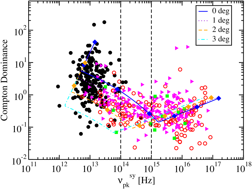
Our modeling results are shown in Figures 6 and 7. The curves show the sources at at constant angle, according to the model, so that along the curve only $B$ and $u_{ext}$ vary according to Equation 11. The model parameters are shown in Table 2, and are fairly close to the values used by Böttcher & Dermer (2002). The sources with low $B$ and low $u_{ext}$ have high $\nu_{pk}^{sy}$, due to the small amount of cooling. As $B$ and $u_{ext}$ increase, the cooling increases, and hence $\gamma_{c}$ decreases. Since $\nu_{pk}^{sy}\propto\epsilon_{pk}\propto\gamma_{c}^{2}B$ (Equation [17]), and $\gamma_{c}$ decreases faster than $B$ increases, $\nu_{pk}^{sy}$ will decrease. If the cooling is great enough, and $\gamma_{c}<\gamma_{1}$, the curves enter the fast cooling regime, and $\nu_{pk}^{sy}$ is associated with $\gamma_{1}$ instead of $\gamma_{c}$ (again Equation [17]). The transition between the fast and slow cooling regimes leads to the sharp break at $\lesssim 10^{13}$ Hz (the exact location depends on the angle) seen in the curves in Figures 6 and 7. In Figure 7, there is also a break in the curves between $\approx 10^{14}$ and $\approx 10^{15}$ Hz caused by the transition between SSC and EC. Note that for SSC, $A_{C}$ does not depend on angle, while for EC, it does. The curves reproduce almost all of the objects in Figures 6 and 7, although there are objects with $A_{C}\lesssim 0.1$ and $\nu_{pk}^{sy}>10^{15}$ Hz that are not reproduced. A possible explanation is if there exist structures within the jet, so that as one views a jet more and more off axis, one views a different region of the jet (Meyer et al., 2011). This would only work if $B$, $Q_{0}$, and/or $R_{b}^{{}^{\prime}}$ also varied not just $\delta_{D}$, since $A_{C}$ is independent of $\delta_{D}$ in the case of SSC.

According to this simple model, all sources have $\Gamma=30$. Of course, in reality, sources will not have jets moving at the same speed, as shown by very long baseline interferometry (VLBI; e.g., Jorstad et al., 2005; Lister et al., 2009; Piner et al., 2008, 2010), which also typically show slower values for $\Gamma$. However, the main emitting regions could be on smaller size scales than is possible to resolve with VLBI, and so may have different speeds, although note that much lower (e.g., Piner et al., 2008) and much higher (e.g., Marscher et al., 2010) Lorentz factors have been observed. It has also been suggested that the jet of a single source may have velocity gradients (e.g., Chiaberge et al., 2000; Stawarz & Ostrowski, 2002; Georganopoulos & Kazanas, 2003; Ghisellini et al., 2005; Meyer et al., 2011). However, we assume a gradient in $\Gamma$ is not necessary to reproduce the general trends (cf. Meyer et al., 2011), and this value may represent an average value for the main emitting region. The magnetic field strength values, which span from $B=0.050$ G to $B=8.6$ G, are consistent with those found from spectral modeling of blazars (e.g., Ghisellini et al., 1998, 2010). These values are also consistent in that the modeling generally shows higher $B$ for FRSQs than BL Lacs.

Blazar SED modeling also indicates that the $\gamma$-ray emission from FSRQs is likely from Compton scattering of an external radiation source, while for HSP BL Lacs SSC is able to provide a good fit to the $\gamma$-ray emission (e.g., Ghisellini et al., 1998, 2010). A correlation between $A_{C}$ and core dominance, a proxy for $\theta$, found in FSRQs, is also evidence that EC dominates in these sources (Meyer et al., 2012). BL Lacs tend to have less prominent “blue bumps” from accretion disks and weaker broad lines, two of the leading contenders for the seed photon source for external Compton scattering. The presumed parent population of BL Lacs, FR I radio galaxies, also seem less likely to have dust tori (Donato et al., 2004), another leading contender for the external photon source. Wide Field Infrared Survey Explorer observations of BL Lacs do not show any evidence for dust tori (Plotkin et al., 2012). So whatever the source is, it seems reasonable to assume it is greater for more FSRQs, and weaker for BL Lacs. This is similar to Böttcher & Dermer (2002) but in contrast to Ghisellini et al., who use a “binary” $u_{ext}$ where the external radiation field is either “on” or “off” above and below a certain accretion rate (e.g., Ghisellini & Tavecchio, 2008a). They justify this from reverberation mapping campaigns, which show the disk luminosity is proportional to the square of the BLR distance from the disk (e.g., Bentz et al., 2006), which would result in the same energy density observed, as long as the emitting region is inside the BLR, and the same fraction of disk emission is reprocessed by the BLR. However, there is no guarantee that this fraction is the same in all sources, or that if the external radiation source is a dust torus that it follows the same relation as the BLR. It seems more likely that $u_{ext}$ can have a range of values, rather than just one. Whether the external photon source is a dust torus or BLR, its luminosity should be less than the Eddington limit for a black hole with mass $M=10^{9}M_{\odot}$, or $L_{Edd}=1.3\times 10^{47}M_{9}\ \mathrm{erg}\ \mathrm{s}^{-1}$ where $M_{9}=M/(10^{9}M_{\odot})$. If the radius of the external source is $R_{ext}=10^{18}\ \mathrm{cm}\approx 1/3\ \mathrm{pc}$, then the maximum energy density will be

$$u_{ext}=\frac{L_{Edd}}{4\pi cR_{ext}^{2}}=0.35\ \mathrm{erg}\ \mathrm{cm}^{-3}\ M_{9}R_{18}^{-2}$$ (23)

where $R_{18}=R_{ext}/(10^{18}\ \mathrm{cm})$. It is unlikely though that the external photon source will be radiating all of the black hole’s accretion luminosity, so $u_{ext}$ should be lower than this by at least a factor 10. We have thus chosen our parameters so that the maximum external energy density is $u_{ext}=0.035\ \mathrm{erg}\ \mathrm{cm}^{-3}$.

We have also computed the jet powers in Poynting flux and electrons, respectively, by

$$P_{j,B}=2\pi R_{b}^{\prime}\Gamma^{2}c\beta u^{\prime}_{B}$$ (24)

and

$$P_{j,e}=2\pi R_{b}^{\prime}\Gamma^{2}c\beta u^{\prime}_{e}\$$ (25)

(Celotti & Fabian, 1993; Celotti et al., 2007; Finke et al., 2008). These results are also shown in Table 3. The jet powers are consistent with those found previously by other authors for spectral modeling (e.g., Ghisellini et al., 2009, 2010). For sources with high $B$, naturally $P_{j,B}$ is higher. In the slow cooling regime, $P_{j,e}$ is nearly independent of $B$ and $u_{ext}$, decreasing with increasing $B$ and $u_{ext}$ only slightly. In the fast cooling regime (Equation [6]), $N_{e}(\gamma)$, and hence $u_{e}$, is directly proportional to $\gamma_{c}$, so that as $B$ and $u_{ext}$ increase, $\gamma_{c}$ decreases, leading to lower $u_{e}$.

Figure 6.— Same as Figure 2, with curves showing our model plotted at various angles, shown in the legend. Along the curves only $B$ and $u_{ext}$ are varied. Model parameters are found in Table 2. Diamond symbols show the location of the model SEDs plotted in Figures 8 and 9, with the numbers indicating the location of the SEDs in Figure 8.

Figure 7.— Same as Figure 5 with curves showing our model plotted at various angles, shown in the legend. Along the curves only $B$ and $u_{ext}$ are varied. Model parameters are found in Table 2. Diamond symbols show the location of the model SEDs plotted in Figures 8 and 9.

Table 2 Parameters (described in the text) for theoretical curves in Figures 6 and 7.

Parameter	Value
$\gamma_{1}$	$10^{2}$
$\gamma_{2}$	$10^{6}$
$R_{b}$	$10^{16}\ \mathrm{cm}$
$\eta$	$1.0$
$L_{inj}$	$2.0\times 10^{42}\ \mathrm{erg}\ \mathrm{s}^{-1}$
$Q_{0}$	$6\times 10^{48}\ \mathrm{s}^{-1}$
$q$	2.5
$u_{0}$	$4.0\times 10^{-11}\ \mathrm{erg}\ \mathrm{cm}^{-3}$
$\Gamma$	$30$
$B_{0}$	$0.05$ G

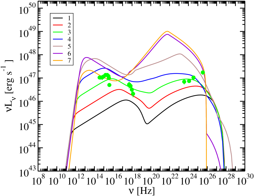
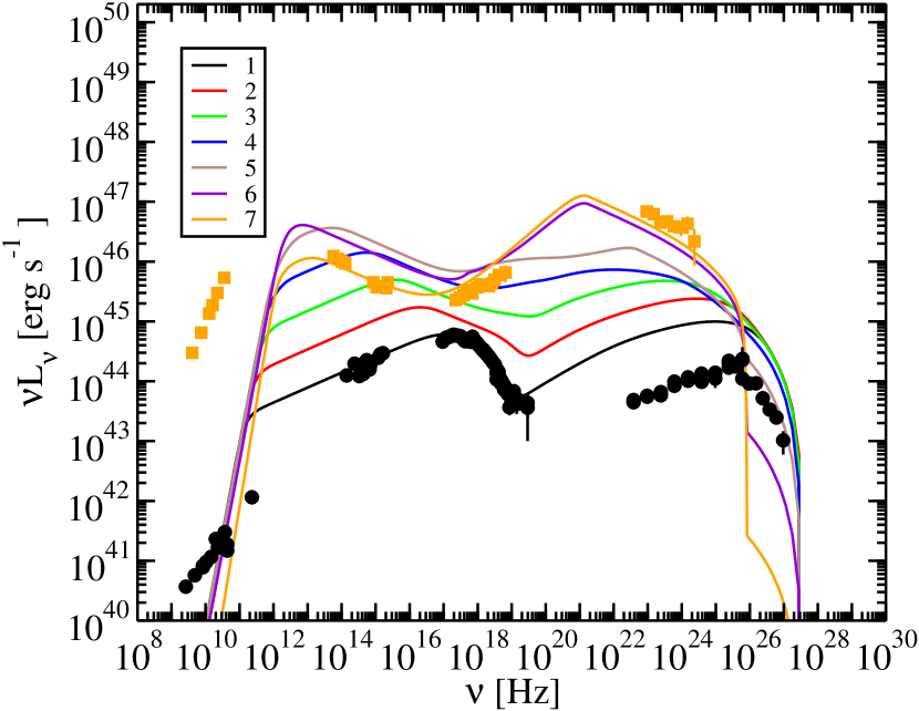
The SEDs of several blazars along the sequence, seen at an angle to the line of sight $\theta=0$ and $\theta=2\arcdeg$ can be seen in Figures 8 and 9, respectively. These SEDs correspond to the diamonds in Figures 6 and 7. The parameters for these curves can be found in Table 3. The external radiation field is assumed to be isotropic in the galaxy’s frame and monochromatic, with dimensionless seed photon energy $\epsilon_{0}=5\times 10^{-7}$ in the galaxy’s frame, which is around what one would expect for the peak emission from a dust torus with temperature $T_{dust}\sim 10^{3}\ \mathrm{K}$. The calculations were performed using the exact synchrotron emissivity and the full Compton cross section, accurate in the Thomson through Klein-Nishina regimes. The details of these calculations can be found in Finke et al. (2008) and Dermer et al. (2009). Since exact expressions are used, the parameters $L_{pk}^{sy}$, $\nu_{pk}^{sy}$, and $A_{C}$ differ slightly from the values found in Figures 6 and 7. Note that synchrotron-self absorption is included in these curves as well, and that it is more apparent for the higher power blazars, where the magnetic field is larger and the emitting region becomes self-absorbed at higher frequencies. A contribution from an underlying accretion disk is not included, although this has been shown to dominate the optical continuum for FSRQs and some BL Lacs. These curves appear similar to SEDs observed from blazars. Similar to Böttcher et al. (2002), we do not attempt to reproduce any individual blazar. However, to demonstrate the similarity to actual blazar SEDs, we plot data for several blazars on these Figures as well. These include the CRATES 0630$-$2406 from Padovani et al. (2012) in Figure 8, and the Mrk 421 SED from Abdo et al. (2011) and the low state 3C 279 from Hayashida et al. (2012), in Figure 9. The symbols have the same color as the curve which is the closest match. The curves are not a perfect fit to the SED data, although they are a reasonable representation.

The scenario described here predicts that a large fraction of FSRQs are emitting in the fast-cooling regime. In this regime ($\gamma_{c}<\gamma_{1}$), one expects the electron index below the peak (associated with $\gamma_{1}$) to be $p=2$, as shown in Equation (6). For FSRQs, Compton scattering by these electrons should make hard X-rays ($\sim$ 10 – 100 keV) and the spectral index from Thomson scattering would then be $\Gamma_{i}=(p+1)/2=1.5$, assuming one is observing reasonably far below the break. In the Swift-BAT spectra from 36 months of observations (Ajello et al., 2009), almost every FSRQ has an X-ray spectral index consistent with $\Gamma_{i}=1.5$ within the error bars, and the mean for the sample is $1.6\pm 0.3$. The BeppoSAX six year catalog (Donato et al., 2005) has a large number of sources are near $\Gamma_{i}\approx 1.5$ with a mean spectral index of $1.59\pm 0.05$, although not all sources in that catalog are consistent with $\Gamma_{i}=1.5$. The diversity of hard X-ray spectral indices could be explained by the location of the Compton component within the BAT or BeppoSAX bandpass. Softer spectra ($\Gamma_{i}>1.5$) could be those with their Compton peak being in or near the BAT or BeppoSAX bandpass, or by a contribution from SSC emission. Harder spectra ($\Gamma_{i}<1.5$) could be caused by the photons scattered by electrons below $\gamma_{c}$ being in the hard X-ray bandpass.

Figure 8.— SEDs for the sequence seen in Figures 6 and 7 as observed at $\theta=0$. The numbers correspond to the numbered diamonds in Figure 6. The circles are the SED data for CRATES 0630$-$2406 from Padovani et al. (2012).

Figure 9.— SEDs for the sequence (diamonds) seen in Figures 6 and 7 as observed at $\theta=2\arcdeg$. The circles are the SED data for Mrk 421 from Abdo et al. (2011), and the squares are the SED data for 3C 279 from Hayashida et al. (2012).

Table 3 Parameters (described in the text) for curves shown in Figures 8 and 9.

Parameter	1	2	3	4	5	6	7
$B$ [G]	$0.050$	$0.12$	$0.28$	$0.67$	$1.6$	$3.8$	$8.6$
$u_{ext}$ [$\mathrm{erg}\ \mathrm{cm}^{-3}$]	$4\times 10^{-11}$	$1.3\times 10^{-9}$	$4.1\times 10^{-8}$	$1.3\times 10^{-6}$	$4.2\times 10^{-5}$	$1.4\times 10^{-3}$	$3.5\times 10^{-2}$
$\gamma_{c}$	$1.4\times 10^{5}$	$3.9\times 10^{4}$	$1.1\times 10^{4}$	$2.7\times 10^{3}$	$5.4\times 10^{2}$	$50$	$2.7$
$P_{j,B}$ [$\mathrm{erg}\ \mathrm{s}^{-1}$]	$1.7\times 10^{42}$	$9.6\times 10^{42}$	$5.4\times 10^{43}$	$3.1\times 10^{44}$	$1.7\times 10^{45}$	$9.8\times 10^{45}$	$5.0\times 10^{46}$
$P_{j,e}$ [$\mathrm{erg}\ \mathrm{s}^{-1}$]	$1.3\times 10^{45}$	$1.3\times 10^{45}$	$1.2\times 10^{45}$	$1.2\times 10^{45}$	$9.5\times 10^{44}$	$4.5\times 10^{44}$	$7.6\times 10^{43}$

4. Summary and Discussion

In Section 2 we have found anti-correlations in the 2LAC that were found previously by many authors in other samples. The plot and correlation with $A_{C}$ in particular is novel, since the 2LAC allows for a larger sample of the Compton component than any previous catalog. We include on this plot for the first time a large number of blazars without known $z$, and showed that the anti-correlation with $\nu_{pk}^{sy}$ is not a relic of ignoring blazars which lack spectroscopic redshifts. This relationship seems to have a physical origin.

Both Meyer et al. (2012) and Ghisellini et al. (2012) plot the LAT $\gamma$-ray luminosity ($L_{\gamma}$) versus the LAT spectral index ($\Gamma_{\gamma}$; a proxy for $\nu_{pk}^{C}$), and showed that the four sources from Padovani et al. (2012) with high $\nu_{pk}^{sy}$, high $L_{pk}^{sy}$ do not have excessively large $L_{\gamma}$ or excessively small $\Gamma_{\gamma}$, and are consistent with other LAT blazars. However, it is possible that the redshifts of many BL Lacs in the future could be measured, and they could be found with high $L_{\gamma}$ and low $\Gamma_{\gamma}$. So it is not possible to assess this selection effect with a plot of $L_{\gamma}$ versus $\Gamma_{\gamma}$.

In Section 3 we developed a simple model to explain the plots and anti-correlations from Section 2. This shape is explained by the increased external radiation field energy density and magnetic field strength, where $\nu_{pk}^{sy}$ is associated with either $\gamma_{c}$ (the Lorentz factor of the break in the electron spectrum due to cooling) for sources in the slow-cooling regime, and $\gamma_{1}$ (the lowest Lorentz factor of the injected electrons) for sources in the fast-cooling regime.

This theory is quite simple, and neglects numerous important effects. Perhaps most importantly, blazars are highly variable, and we treat them with a steady-state solution to the electron continuity equation. In any study of a large population of blazars, however, this is almost unavoidable. In developing this theory, approximate expressions were used, neglecting the exact synchrotron emissivity and Compton cross section, especially Klein-Nishina effects. However, a comparison between the predictions and exact calculations (Figure 8) shows that these approximations seem reasonable.

Despite its simplicity, this model makes a number of predictions. It predicts that the single most important parameter in determining the luminosity ($L_{pk}^{sy}$) of blazars is $\theta$, mostly independent of the frequency of their synchrotron peak (Figure 6). This also means that as fainter sources are found, these sources will not have excessively large values for $A_{C}$, since large values for this quantity are due to EC, and $A_{C}$ is strongly dependent on $\theta$ if EC is dominant. There should not be any sources found with $L_{pk}^{sy}\lesssim 10^{45}\ \mathrm{erg}\ \mathrm{s}^{-1}$ and $A_{C}\gtrsim$ a few. This model also predicts that no “blue FSRQs”, that is, no HSPs with significant BLR or dust torus luminosity will be found. It predicts that any source with high $A_{C}$ ($\gtrsim$ a few) will be an LSP and it will be in the fast cooling regime, so that the spectral index of the EC emission below the $\gamma$-ray peak will be $\Gamma_{i}\sim 1.5$. For most sources, this will be in the soft $\gamma$-rays ($\lesssim 10$ MeV) down to the hard X-ray regime, perhaps as low as 10 keV in some cases.

This model predicts that if the BL Lacs sources become more redshift-complete, more sources with high $L_{pk}^{sy}$ and $\nu_{pk}^{sy}$ (“bright HSPs”) will be found, although these sources will not be as bright as the brightest LSPs (Figure 6). These sources will have their jets highly aligned with our line of sight. Note that our scenario differs somewhat from the one of Ghisellini et al. (2012). They also predict that bright HSP sources will be found, but in their case, these sources are “blue FSRQs”, with the primary emitting region found outside the BLR, avoiding an EC component and a large $A_{C}$, since the $\gamma$-ray emission will be due only to SSC. Their scenario and ours would produce essentially identical SEDs for bright HSPs, so distinguishing them is not possible based on SEDs alone. If it could be found that these sources have their jets highly aligned, that they do not have significant BLRs or dust tori, or that the BLRs are not the seed photon sources for EC in “red” (i.e., LSP) FSRQs, it would favor our scenario. All of these things are difficult to determine observationally, however. The nonthermal synchrotron makes broad emission lines or a dust component nearly impossible to observe, although jet alignment may be possible to determine with VLBI observations (e.g., Jorstad et al., 2005).

Our model can also be contrasted with the Monte Carlo simulations of Giommi et al. (2012a). In their simulations, they randomly draw for each blazar several properties including $\gamma_{pk}$ (the peak of the electron distribution) $\delta_{D}$, and the strength of the broad emission lines, all independent of each other. Although they do not explore the Compton dominance in their paper, if these properties are in reality independent of each other, and if the BLR is the seed photon source for Compton scattering, the scenario of Giommi et al. (2012a) would not produce a correlation between $A_{C}$ and $\nu_{pk}^{sy}$, and would produce objects with high $A_{C}$ and high $\nu_{pk}^{sy}$. Since no such objects are found (Figure 5) and a correlation between $A_{C}$ and $\nu_{pk}^{sy}$ is found (Table 1), their scenario does not seem to be in agreement with observations.

Our simple model assumes the primary emitting region has a single Lorentz factor. Based on optical (Chiaberge et al., 2000) and $\gamma$-ray (Abdo et al., 2010b, a) observations of radio galaxies, it seems highly likely that jets are stratified in speed either perpendicular (Stawarz & Ostrowski, 2002; Ghisellini et al., 2005) or parallel to the jet’s direction of motion (Georganopoulos & Kazanas, 2003). Indeed, Meyer et al. (2011) have an explanation for an “L” shape in a plot of $L_{pk}^{sy}$ versus $\nu_{pk}^{sy}$, based on sources with varying Lorentz factors within a source. In our study we neglect radio galaxies and stratified jets. However, modeling of radio galaxies (Chiaberge et al., 2001; Abdo et al., 2009c, 2010c; Migliori et al., 2011) indicates that these types of structures almost certainly exist. Whether they can explain the properties of blazars as well as radio galaxies remains to be seen.

Another possible way to decipher the correct model could involve estimating the power injected into the jet. This power can be related to the power needed to create a cavity in the hot X-ray emitting ICM surrounding radio galaxies (Bîrzan et al., 2004, 2008; Cavagnolo et al., 2010). This power seems to be correlated with the extended lobe’s radio power, and Meyer et al. (2011) have used the radio power as a proxy for jet kinetic power. This angle-independent measure of the jet kinetic power may provide a way of distinguishing viewing angle effects from intrinsic power effects.

As a redshift-independent quantity, the Compton dominance is a useful tool for exploring blazar properties, including the large number of BL Lacs without known redshifts. The large new blazar catalog from the Fermi-LAT is able to characterize the Compton component for a larger number of objects than previously possible, making it valuable for determining its relationship to the blazar sequence.

References

- Abdo et al. (2009a) Abdo, A. A., et al. 2009a, ApJ, 700, 597
- Abdo et al. (2009b) —. 2009b, ApJ, 699, 817
- Abdo et al. (2009c) —. 2009c, ApJ, 707, 55
- Abdo et al. (2010a) —. 2010a, ApJ, 720, 912
- Abdo et al. (2010b) —. 2010b, ApJ, 719, 1433
- Abdo et al. (2010c) —. 2010c, ApJ, 710, 1271
- Abdo et al. (2011) —. 2011, ApJ, 736, 131
- Ackermann et al. (2011) Ackermann, M., et al. 2011, ApJ, 743, 171
- Aharonian et al. (2007) Aharonian, F., et al. 2007, ApJ, 664, L71
- Ajello et al. (2009) Ajello, M., et al. 2009, ApJ, 699, 603
- Bentz et al. (2006) Bentz, M. C., Peterson, B. M., Pogge, R. W., Vestergaard, M., & Onken, C. A. 2006, ApJ, 644, 133
- Bîrzan et al. (2008) Bîrzan, L., McNamara, B. R., Nulsen, P. E. J., Carilli, C. L., & Wise, M. W. 2008, ApJ, 686, 859
- Bîrzan et al. (2004) Bîrzan, L., Rafferty, D. A., McNamara, B. R., Wise, M. W., & Nulsen, P. E. J. 2004, ApJ, 607, 800
- Blandford & Znajek (1977) Blandford, R. D., & Znajek, R. L. 1977, MNRAS, 179, 433
- Böttcher & Dermer (2002) Böttcher, M., & Dermer, C. D. 2002, ApJ, 564, 86
- Böttcher et al. (1997) Böttcher, M., Mause, H., & Schlickeiser, R. 1997, A&A, 324, 395
- Böttcher et al. (2002) Böttcher, M., Mukherjee, R., & Reimer, A. 2002, ApJ, 581, 143
- Cavagnolo et al. (2010) Cavagnolo, K. W., McNamara, B. R., Nulsen, P. E. J., Carilli, C. L., Jones, C., & Bîrzan, L. 2010, ApJ, 720, 1066
- Cavaliere & D’Elia (2002) Cavaliere, A., & D’Elia, V. 2002, ApJ, 571, 226
- Celotti & Fabian (1993) Celotti, A., & Fabian, A. C. 1993, MNRAS, 264, 228
- Celotti et al. (2007) Celotti, A., Ghisellini, G., & Fabian, A. C. 2007, MNRAS, 375, 417
- Chen & Bai (2011) Chen, L., & Bai, J. M. 2011, ApJ, 735, 108
- Chiaberge et al. (2001) Chiaberge, M., Capetti, A., & Celotti, A. 2001, MNRAS, 324, L33
- Chiaberge et al. (2000) Chiaberge, M., Celotti, A., Capetti, A., & Ghisellini, G. 2000, A&A, 358, 104
- Costamante et al. (2001) Costamante, L., et al. 2001, A&A, 371, 512
- Dermer (1995) Dermer, C. D. 1995, ApJ, 446, L63+
- Dermer et al. (2000) Dermer, C. D., Chiang, J., & Mitman, K. E. 2000, ApJ, 537, 785
- Dermer et al. (2009) Dermer, C. D., Finke, J. D., Krug, H., & Böttcher, M. 2009, ApJ, 692, 32
- Dermer & Menon (2009) Dermer, C. D., & Menon, G. 2009, High Energy Radiation from Black Holes: Gamma Rays, Cosmic Rays, and Neutrinos, ed. Dermer, C. D. & Menon, G.
- Dermer & Schlickeiser (2002) Dermer, C. D., & Schlickeiser, R. 2002, ApJ, 575, 667
- Donato et al. (2004) Donato, D., Sambruna, R. M., & Gliozzi, M. 2004, ApJ, 617, 915
- Donato et al. (2005) —. 2005, A&A, 433, 1163
- Fanaroff & Riley (1974) Fanaroff, B. L., & Riley, J. M. 1974, MNRAS, 167, 31P
- Finke et al. (2008) Finke, J. D., Dermer, C. D., & Böttcher, M. 2008, ApJ, 686, 181
- Fossati et al. (1998) Fossati, G., Maraschi, L., Celotti, A., Comastri, A., & Ghisellini, G. 1998, MNRAS, 299, 433
- Fossati et al. (2000) Fossati, G., et al. 2000, ApJ, 541, 166
- Georganopoulos & Kazanas (2003) Georganopoulos, M., & Kazanas, D. 2003, ApJ, 594, L27
- Georganopoulos et al. (2001) Georganopoulos, M., Kirk, J. G., & Mastichiadis, A. 2001, ApJ, 561, 111
- Ghisellini et al. (1998) Ghisellini, G., Celotti, A., Fossati, G., Maraschi, L., & Comastri, A. 1998, MNRAS, 301, 451
- Ghisellini & Tavecchio (2008a) Ghisellini, G., & Tavecchio, F. 2008a, MNRAS, 386, L28
- Ghisellini & Tavecchio (2008b) —. 2008b, MNRAS, 387, 1669
- Ghisellini et al. (2005) Ghisellini, G., Tavecchio, F., & Chiaberge, M. 2005, A&A, 432, 401
- Ghisellini et al. (2010) Ghisellini, G., Tavecchio, F., Foschini, L., Ghirlanda, G., Maraschi, L., & Celotti, A. 2010, MNRAS, 402, 497
- Ghisellini et al. (2012) Ghisellini, G., Tavecchio, F., Foschini, L., Sbarrato, T., Ghirlanda, G., & Maraschi, L. 2012, MNRAS, in press, arXiv:1205.0808
- Ghisellini et al. (2009) Ghisellini, G., Tavecchio, F., & Ghirlanda, G. 2009, MNRAS, 399, 2041
- Giommi et al. (2002) Giommi, P., Padovani, P., Perri, M., Landt, H., & Perlman, E. 2002, in Blazar Astrophysics with BeppoSAX and Other Observatories, ed. P. Giommi, E. Massaro, & G. Palumbo, 133–+
- Giommi et al. (2012a) Giommi, P., Padovani, P., Polenta, G., Turriziani, S., D’Elia, V., & Piranomonte, S. 2012a, MNRAS, 420, 2899
- Giommi et al. (2005) Giommi, P., Piranomonte, S., Perri, M., & Padovani, P. 2005, A&A, 434, 385
- Giommi et al. (2012b) Giommi, P., et al. 2012b, A&A, 541, A160
- Hardcastle et al. (2007) Hardcastle, M. J., Evans, D. A., & Croston, J. H. 2007, MNRAS, 376, 1849
- Hayashida et al. (2012) Hayashida, M., et al. 2012, ApJ, 754, 114
- Jorstad et al. (2005) Jorstad, S. G., et al. 2005, AJ, 130, 1418
- Landt et al. (2004) Landt, H., Padovani, P., Perlman, E. S., & Giommi, P. 2004, MNRAS, 351, 83
- Lister et al. (2009) Lister, M. L., et al. 2009, AJ, 138, 1874
- Lister et al. (2011) —. 2011, ApJ, 742, 27
- Marcha et al. (1996) Marcha, M. J. M., Browne, I. W. A., Impey, C. D., & Smith, P. S. 1996, MNRAS, 281, 425
- Marscher et al. (2010) Marscher, A. P., et al. 2010, ApJ, 710, L126
- Meyer et al. (2011) Meyer, E. T., Fossati, G., Georganopoulos, M., & Lister, M. L. 2011, ApJ, 740, 98
- Meyer et al. (2012) —. 2012, ApJ, 752, L4
- Migliori et al. (2011) Migliori, G., et al. 2011, A&A, 533, A72
- Nieppola et al. (2006) Nieppola, E., Tornikoski, M., & Valtaoja, E. 2006, A&A, 445, 441
- Padovani (2007) Padovani, P. 2007, Ap&SS, 309, 63
- Padovani et al. (2002) Padovani, P., Costamante, L., Ghisellini, G., Giommi, P., & Perlman, E. 2002, ApJ, 581, 895
- Padovani et al. (2012) Padovani, P., Giommi, P., & Rau, A. 2012, MNRAS, 422, L48
- Padovani et al. (2003) Padovani, P., Perlman, E. S., Landt, H., Giommi, P., & Perri, M. 2003, ApJ, 588, 128
- Piner et al. (2008) Piner, B. G., Pant, N., & Edwards, P. G. 2008, ApJ, 678, 64
- Piner et al. (2010) —. 2010, ApJ, 723, 1150
- Plotkin et al. (2012) Plotkin, R. M., Anderson, S. F., Brandt, W. N., Markoff, S., Shemmer, O., & Wu, J. 2012, ApJ, 745, L27
- Rau et al. (2012) Rau, A., et al. 2012, A&A, 538, A26
- Schlickeiser (2009) Schlickeiser, R. 2009, MNRAS, 398, 1483
- Schlickeiser et al. (2010) Schlickeiser, R., Böttcher, M., & Menzler, U. 2010, A&A, 519, A9+
- Sikora et al. (2009) Sikora, M., Stawarz, Ł., Moderski, R., Nalewajko, K., & Madejski, G. M. 2009, ApJ, 704, 38
- Stawarz & Ostrowski (2002) Stawarz, Ł., & Ostrowski, M. 2002, ApJ, 578, 763
- Urry & Padovani (1995) Urry, C. M., & Padovani, P. 1995, PASP, 107, 803
- Zacharias & Schlickeiser (2010) Zacharias, M., & Schlickeiser, R. 2010, A&A, 524, A31+
- Zacharias & Schlickeiser (2012) —. 2012, MNRAS, 420, 84