SLAC-PUB-15306 Dichromatic Dark Matter

Abstract

Both the robust INTEGRAL 511 keV gamma-ray line and the recent tentative hint of the 135 GeV gamma-ray line from Fermi-LAT have similar signal morphologies, and may be produced from the same dark matter annihilation. Motivated by this observation, we construct a dark matter model to explain both signals and to accommodate the two required annihilation cross sections that are different by more than six orders of magnitude. In our model, to generate the low-energy positrons for INTEGRAL, dark matter particles annihilate into a complex scalar that couples to photon via a charge-radius operator. The complex scalar contains an excited state decaying into the ground state plus an off-shell photon to generate a pair of positron and electron. Two charged particles with non-degenerate masses are necessary for generating this charge-radius operator. One charged particle is predicted to be long-lived and have a mass around 3.8 TeV to explain the dark matter thermal relic abundance from its late decay. The other charged particle is predicted to have a mass below 1 TeV given the ratio of the two signal cross sections. The 14 TeV LHC will concretely test the main parameter space of this lighter charged particle.

1 Introduction

Although dark matter serves as the dominant component of matter in our universe, its various properties remain unknown. From astrophysical evidence, there is no doubt that dark matter can interact with the Standard Model (SM) particles through gravitational interaction. However, whether there are additional interactions between dark matter and SM particles is still a mystery to us. Among several approaches to search for dark matter particles, measuring the cosmic ray spectrum provides the indirect detection of dark matter. Observing a high-energy gamma-ray line has long been believed to be the “smoking gun” of the dark matter detection [1, 2, 3, 4, 5, 6]. Furthermore, the propagation of energetic photons in our Galaxy is less affected by the interstellar gas or Galactic magnetic field. The gamma-ray line signal can even provide the dark matter geometrical profile in our Galaxy.

The detection of celestial gamma-ray line at $511$ keV from the inner galaxy, which is believed to be caused by $e^{+}e^{-}$ annihilations, was first reported by [7] and later confirmed by [8, 9, 10, 11]. The total flux of the 511 keV line has been estimated to be around $2\times 10^{-3}~{}{\rm cm^{-2}~{}s^{-1}}$ [12]. About $97\%$ $e^{+}e^{-}$ annihilations proceed through the intermediate state of a positronium atom, and 25$\%$ of these annihilations with opposite spin of $e^{+}$ and $e^{-}$ can produce 511 keV line emission [13, 14]. Although this gamma-ray line has been known for decades, the identification of the positron source remains undetermined. Different astrophysical sources have been suggested during the years, but each of the models faces various challenge to explain the observations consistently. The relatively high ratio of the bulge to disk 511 keV emission towards the inner Galaxy seems against its origin from hypernovae and gamma ray bursts, while the constraints on the production rate of high energy positrons also disfavors millisecond pulsars, as well as proton-proton collisions from e.g. microquasars, low luminosity X-ray binary jets, and the central supermassive black hole. Furthermore, pulsars, magnetars, and Galactic cosmic rays are not favored as major sources to the observed 511 keV from the bulge, and stringent constraints on these origin of the 511 keV line was suggested [15, 16].

Besides these astrophysical suggestions, the possibility that dark matter may create the 511 keV gamma-ray line has been widely discussed, mainly motivated by the rather spheroidal, symmetric, bulge-centered morphology. The lack of higher energy gamma ray requires the injection energy of positrons to be below $\sim$ 3 MeV [15]. This motivates studies for both MeV-scale dark matter models [17, 18, 19, 20, 21, 22] and TeV-scale dark matter models with a MeV mass splitting among different dark matter states [23, 24, 25, 26]. Since TeV-scale dark matter with electroweak interaction strength can naturally gives correct thermal relic abundance, those models are more favored. Interestingly, the morphology of the 511 keV signal profile has a peaked structure around the Galactic center, and the sharpness of the peak prefers to have dark matter annihilation rather than decaying as an explanation [12]. Thus we focus on the heavy dark matter scenario, and try to explain the $511$ keV INTEGRAL signal via dark matter annihilation.

One popular dark matter model to explain the INTEGRAL signal is the excited dark matter model with an MeV mass splitting [24]. This class of models suffer from the requirement of a large kinematic energy of dark matter to excite the ground state, hence relying on the Boltzmann tail of dark matter velocity distribution. It is under a debate whether the excited dark matter model can generate enough positrons to explain the large gamma-ray flux for the INTEGRAL data [27, 28]. For the 100 GeV dark matter mass region that we will consider in this paper, the situation is worse, because it requires a higher velocity to obtain enough kinematic energy comparing to a TeV mass dark matter. In our paper, we will address this problem and propose a new scenario of the Down-scattering excited Dark Matter (DeDM) to solve the Boltzmann suppression problem of the vanilla excited dark matter models.

More recently, the hint for another gamma-ray line around 130 GeV from the Galactic center has been suggested by analyzing the public data from Fermi Gamma-ray Space Telescope (Fermi-LAT) [29, 30]. The hint becomes even stronger with the template fitting approach, which takes into account the spatial distribution of the LAT events towards the inner Galaxy along with the spectral information [31]. Fermi-LAT Collaboration has confirmed the hint of the peak at $\sim 130$ GeV using Pass 7 data. The peak shifts to a higher mass at $\sim 135$ GeV and the significance becomes weaker using the reprocessed Pass 7 data [32]. Such high energy gamma-ray line emission has been considered as a clean signature from dark matter annihilations. Many dark matter models have been constructed to explain the 130(135) GeV gamma-ray line feature (see [33] and references therein).

The morphology of the INTEGRAL 511 keV and Fermi-LAT 130(135) GeV line shares similar structures: (1) the signal events concentrate at the center of the Galaxy with non-disk like distributions; (2) after smoothing Fermi-LAT signal with INTEGRAL’s angular resolution, they have comparable full widths at half maximum (FWHM) in both the longitudinal and latitude directions. This motivates us to explain both signals using same dark matter particle in our universe. The fittings for both signals prefer annihilation rather than decaying [12, 34]. Having worked out the required annihilation cross sections, we find that the INTEGRAL 511 keV cross section is six to seven orders of magnitude larger than that of the Fermi-LAT 130 GeV line. This large hierarchy of cross sections sets a challenge when constructing a detailed model. However, the order of magnitude is comparable with an electromagnetic loop factor of ${\cal O}(\alpha^{2}/\pi^{2})$ if the INTEGRAL and Fermi-LAT signals are coming from tree-level and loop-level processes, respectively. This serves as a clue for our model building.

Our paper is organized as following. In $\S$2, we emphasize the similarities of morphologies for both signals and work out the required cross sections. In $\S$3, we propose our model, Down-scattering excited Dark Matter model, to explain both signals. In section $\S$3.1, we first provide a general operator analysis to illustrate the essence of our model and calculate the scales of cutoffs of the effective operators. Then we build up a concrete UV-completion for the operator analysis in $\S$3.2. In $\S$3.3, we discuss the thermal history of our model. One charged particle needs to be long-lived in our UV model, so that we have a semi-natural model to explain the final dark matter relic abundance.

2 Experimental Data

In this section, we discuss the INTEGRAL and Fermi-LAT oberservations in more detail. Since photon is not much affected during its propagation in the Galaxy, photon coming from dark matter annihilation can be used to determine the dark matter distribution in our Galaxy. However, there are subtleties on how to map the INTEGRAL 511 keV gamma-ray line signal profile to the dark matter distribution profile. This is because the low-energy positrons that are generated from dark matter particles can propagate through the interstellar medium and annihilate with electrons to photons away from the production site and bias the inferred dark matter distribution from the 511 keV line morphology. In this paper, we assume that the positron propagation is negligible comparing to the spatial resolution of the INTEGRAL, thus the dark matter profile can be estimated by measuring 511 keV emission morphology. On the other hand, the Fermi-LAT 130(135) GeV photons could directly be generated from dark matter particles, and its morphology can therefore tell us the dark matter profile.

We first compare the morphologies of the INTEGRAL $511$ keV and Fermi-LAT 130(135) GeV lines. After smoothing the Fermi-LAT 130(135) GeV line using the angular resolution of INTEGRAL, we find the spatial distributions are comparable to each other. Furthermore, assuming that both signals are generated by dark matter annihilation, we estimate the annihilation cross sections for the two processes. They will serve as inputs for our model building in the rest of the paper.

2.1 Experimental Data

Thanks to a coded mask located $1.7$ m above the detector plane and a specific dithering observational strategy, the spectrometer (SPI) onboard the INTEGRAL observatory can image the sky with a spatial resolution of $\sim$ 2.6^∘ (FWHM). Based on observations recorded from February $22nd$, 2003 to January, 2$nd$ 2009, the study in [35] has obtained the morphology of the 511 keV line towards the inner Galaxy. In Figure 1, we compare the intensity of the 511 keV gamma-ray line as a function of Galactic longitude and latitude with the 130 GeV line profile obtained by fitting 3.7 years Fermi-LAT observations [36]. Especially, the dark green line shows the 130 GeV line profile further smoothed by SPI 2.6^∘ FWHM beam.

Interestingly, both longitudinal and latitude distributions of INTEGRAL are comparable to those of Fermi-LAT after smoothing. Furthermore, both distributions show the tendency to be off-center in the negative longitudinal direction[31, 35]. These similarities motivate the attempts to build one dark matter model to explain both these two signals.

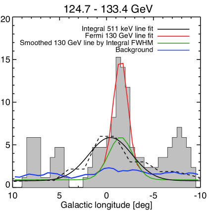
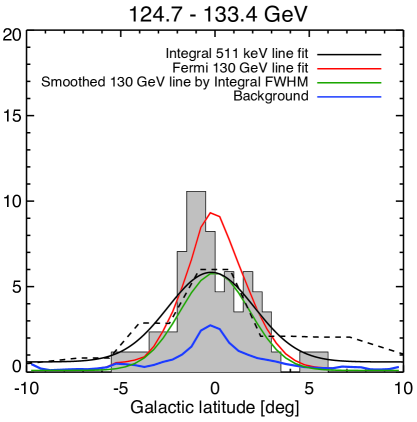
Figure 1: Comparison of the INTEGRAL 511 keV line profile [35] and Fermi-LAT 130 GeV line profile [36] from the Galacitc center, on longitudinal (left) and latitudinal (right) projections. The black dashed line shows the 511 keV line profile measured by INTEGRAL, and the black solid line shows the fitted Gaussian. The shaded histogram shows the 130 GeV line profile from 3.7 years of Fermi-LAT data. The red solid line shows the best fitted Gaussian of the 130 GeV line, which is the same as Fig. 15 in [31]. The green solid line illustrates the 130 GeV line profile smoothed by SPI 2.6^∘ FWHM beam. For the INTEGRAL data, the vertical axis has an arbitrary scale in this plot.

2.2 Dark matter annihilation cross sections for INTEGRAL and Fermi-LAT

As discussed in the previous section, both the 511 keV line and the Fermi-LAT 130(135) GeV line could potentially be explained by dark matter annihilation. In this section, we estimate the required annihilation cross sections for both experiments.

The gamma-ray line intensity in a given direction provided by dark matter annihilation is the line-of-sight integral of the squared dark matter number density along that given direction

$$\frac{d\Phi_{\gamma}}{dE_{\gamma}}=d_{\rm\chi}\,N_{\rm conv}\,\frac{N_{e^{+}/\gamma}\,\langle\sigma v_{r}\rangle_{e^{+}/\gamma}}{2}\,\frac{R_{\odot}\,\rho_{\odot}^{2}\,J}{4\pi\,m_{\chi}^{2}}\,\delta(E-E_{\gamma})\,,$$ (1)

with the $J$-factor defined as:

$$J=\int db\int d\ell\int\frac{ds}{R_{\odot}}\,\cos{b}\,\left[\frac{\rho(r)}{\rho_{\odot}}\right]^{2},$$ (2)

where $l$ and $b$ are longitude and latitude, and the integral of $s$ is along the line of sight. Here, $R_{\odot}\simeq 8.5$ kpc is the distance from the Sun to the galactic center; $\rho(r)$ is the dark matter halo profile; $\rho_{\odot}\simeq 0.4$ GeV cm^-3 is the often-used dark matter density in the Solar system [37]; the relation between $r$ and $s$ is $r^{2}=s^{2}+R_{\odot}^{2}-2sR_{\odot}\cos\ell\cos b$; $N_{\gamma}$ ($N_{e^{+}}$) is the number of photons (positrons) generated from each dark matter annihilation hard process; $m_{\chi}$ is the dark matter mass; $\langle\sigma v_{r}\rangle_{e^{+}}$ and $\langle\sigma v_{r}\rangle_{\gamma}$ are the annihilation cross sections. We define $d_{\rm\chi}=1$ for self-conjugated dark matter, e.g. a real scalar or a Majorana fermion, and $d_{\rm\chi}=\frac{1}{2}$ for a complex scalar or a Dirac fermion. $N_{\rm conv}$ is the number of monochromatic photons that the final states could convert to. For Fermi-LAT, $N_{\rm conv}=1$, since we assume that only monochromatic photons are produced in the hard process. For INTEGRAL, observations suggest that about $97\%$ of positrons annihilate through positronium formation [38]. Only 1/4 of annihilation takes place in the parapositronium state, which produces two 511 keV photons. So, we have $N_{\rm conv}\approx 0.55$ for INTEGRAL.

We consider both the Einasto and the Navarro-Frenk-White (NFW) dark matter profile

$$\rho_{\rm{}_{Ein}}(r)=\rho_{\odot}\,e^{-\frac{2}{\alpha}\left[\left(\frac{r}{r_{s}}\right)^{\alpha}-\left(\frac{r_{\odot}}{r_{s}}\right)^{\alpha}\right]}\,,\qquad\qquad\rho_{\rm{}_{NFW}}(r)=\rho_{\odot}\,\left(\frac{r_{\odot}}{r}\right)^{\alpha}\,\left[\frac{1+r_{\odot}/r_{s}}{1+r/r_{s}}\right]^{3-\alpha}\,,$$ (3)

with $r_{s}=20$ kpc and $\alpha=0.17$ for Einasto [39] and $\alpha=1$ for NFW [40]. Using the fitted fluxes for the INTEGRAL signal (the dark matter+disk ones) in Ref. [41], we obtain the annihilation cross sections as 

$$\langle\sigma v_{r}\rangle_{\gamma,\rm 511,Ein(NFW)}=\,\frac{1}{d_{\rm\chi}N_{e^{+}}}\,\times\,1.5(0.28)\,\times 10^{5}\times\left(\frac{m_{\chi}}{100~{}{\rm GeV}}\right)^{2}~{}\mbox{pb}\cdot{c}\,.$$ (4)

For the Fermi-LAT 130(135) GeV gamma line, we use the fitted fluxes from Ref. [29] for both profiles to calculate the cross sections,

$$\langle\sigma v_{r}\rangle_{\gamma,\rm 135,Ein(NFW)}=\,\frac{1}{d_{\rm\chi}N_{\gamma}}\,\times\,0.42(0.76)\,\times 10^{-1}\times\left(\frac{m_{\chi}}{100~{}{\rm GeV}}\right)^{2}~{}\mbox{pb}\cdot{c}\,.$$ (5)

To quantify the ratio of the required cross sections for two experimental results, we define $R^{135}_{511}\equiv\langle\sigma v_{r}\rangle_{\gamma,\rm 135}/\langle\sigma v_{r}\rangle_{\gamma,\rm 511}$. Taking $N_{e^{+}}=N_{\gamma}=2$, we have the experimentally measured ratios as

$$(R^{135}_{511})_{\rm exp,Ein}\approx 2.9\times 10^{-7}\,,\qquad\quad(R^{135}_{511})_{\rm exp,NFW}\approx 2.7\times 10^{-6}\,,$$ (6)

where clearly show a large hierarchy for the two required cross sections. We want to also stress that the astrophysical uncertainties are fairly large and a global fit by combining the INTEGRAL and Fermi-LAT might bring the uncertainty down. The cross section ratio between these two expertiments is ${\cal O}(10^{-6}\sim 10^{-7})$. This will be the input for model building in latter sections. Interestingly, this ratio is comparable to the square of the electromagnetic loop factor $(\alpha^{2}/\pi^{2})\sim 6\times 10^{-6}$, which implies these two experimental results may be related by a loop with two electromagnetic vertices. It serves as a clue for model building.

3 Down-scattering excited Dark Matter

There are several interesting features required to construct dark matter models if both signatures are to be explained by the same dark matter particle with a mass at the 100 GeV scale.

• The required cross section for the INTEGRAL data is amazingly large. For a simplest estimation on the annihilation rate, we get $\sigma v\sim 1/(4\pi\,m^{2}_{\chi})\sim 3\times 10^{3}$ $\mbox{pb}\cdot{c}$ for $m_{\chi}$ around 100 GeV. This estimation is three orders of magnitude smaller than the required one. Additional mechanisms are therefore required to increase the annihilation rate. There are several ways to achieve this and we pay special attention on the resonance enhancement [42, 43, 44, 45, 46, 47].

• To explain the INTEGRAL data, primary positron injections from dark matter are required. Since we don’t see any excess for other cosmic rays, the underlying dark matter model should be arranged to treat positron/electron differently from other particles. In principle, this can be achieved either from kinematic constraints or symmetry reasons.

• The ratio of the two cross sections is $\langle\sigma v_{r}\rangle_{\rm 135}/\langle\sigma v_{r}\rangle_{\rm 511}\sim 10^{-7}\$or$\ 10^{-6}$. The dark matter model should also provide a natural explanation for this hierarchy of two cross sections.

• The model should provide correct amount of dark matter relic abundance to be consistent with observation.

In the following, we will provide a particle physics model to incorporate all above four ingredients. Specifically, we will use a resonance particle in the $s$-channel to increase the dark matter annihilation cross section required for 511 keV gamma-ray line. The kinematic constraints from a small mass splitting will be used in this paper to select positron/electron as the signals from dark matter annihilation. Instead of introducing a light mediator, e.g. dark photon, for the dark matter sector connecting to the positron/electron, we use photon as a more natural mediator to achieve this goal. Noticing that a neutral scalar field cannot decay into another neutral scalar field plus one on-shell photon, which is the reason why $\Upsilon[(n+1)S]\nrightarrow\Upsilon[nS]+\gamma$, a neutral scalar coupling to photon with the charge-radius operator can naturally induce $e^{\pm}$ without generating a photon signal in the meanwhile. The mass difference of the two scalar fields is chosen to be small such that the kinematic energy of $e^{\pm}$ is small enough to be consistent with observation. To explain the ratio of the cross sections, we will have the cross section for INTEGRAL to be controlled by coefficients of renormalizable operators, while loop-generated higher-dimensional operators for Fermi-LAT. We will first perform an operator analysis and then provide a UV-complete model.

3.1 Operator analysis

We introduce one Dirac fermion $\chi$ and one complex scalar field $\Phi\equiv(\phi_{1}+i\phi_{2})/\sqrt{2}$ in the dark matter sector. Both $\chi$ and $\phi_{1}$ are stable particles and coexist in our current Universe. In our study, we will assume that the dark matter component $\chi$ occupies the majority of the dark matter energy, but we will come back to discuss the relative relic abundances of them later. The interactions of the dark matter sector to the SM particles are described by the following set of effective operators

$$-{\cal L}\supset i\,\lambda_{\chi}\,\overline{\chi}\gamma^{5}\chi\,S+\mu\,S\,\Phi^{\dagger}\Phi\,+\,\frac{\lambda_{S}\,\alpha}{4\pi\,M}\,S\,F_{\mu\nu}F^{\mu\nu}\,+\,\frac{\lambda_{\Phi}\,e}{16\pi^{2}\,M^{2}}\,\partial_{\mu}\Phi\partial_{\nu}\Phi^{\dagger}F^{\mu\nu}\,,$$ (7)

where we implicitly assume that the higher-dimensional operators can be generated at one-loop level. The annihilation of $\chi$’s is through exchanging the real scalar $S$ in the $s$-channel. For the INTEGRAL data, a small mass scale at around 1 MeV is required to generate positrons almost at rest. In our model, we introduce this small mass scale as the mass splitting of $\phi_{1}$ and $\phi_{2}$ from $\Phi=(\phi_{1}+\phi_{2})/\sqrt{2}$ such that $\delta\equiv m_{\phi_{2}}-m_{\phi_{1}}\ll m_{\phi_{1}}$ and $\delta\sim 1$ MeV. Noticing that the parameter $\delta$ explicitly breaks the global $U(1)_{\phi}$, so the smallness of $\delta$ is technically natural. Expanding the last operator in terms of $\phi_{1}$ and $\phi_{2}$, we have

$$\frac{\lambda_{\Phi}\,e}{16\pi^{2}\,M^{2}}\,i\,\partial_{\mu}\phi_{2}\partial_{\nu}\phi_{1}F^{\mu\nu}\,.$$ (8)

Using the equation of motion, one can rewrite the above operator as $\phi_{2}\partial{{}_{\nu}}\phi_{1}\partial_{\mu}F^{\mu\nu}=\phi_{2}\partial{{}_{\nu}}\phi_{1}j^{\nu}$. This indicates that $\phi_{2}$ cannot decay to a mass-on-shell photon. For $2\,m_{e}<\delta<2\,m_{\mu}$, we have the leading decay channel of $\phi_{2}$ as

$$\phi_{2}\rightarrow\phi_{1}\,+\,\gamma^{*}\rightarrow\phi_{1}\,+\,e^{+}\,+\,e^{-}\,.$$ (9)

Photon, naturally, behaves as a mediator for the dark matter sector to generate positrons.

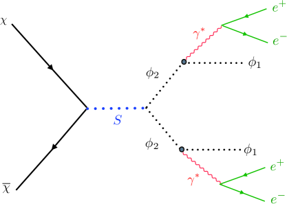
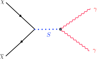
Figure 2: The Feynman diagrams for INTEGRAL (left) and Fermi-LAT (right).

The processes to generate positrons for INTEGRAL and photons for Fermi-LAT are shown in Fig. 2, where the solid thick points indicate higher-dimensional operators for those vertices. Although it looks like that the relative cross sections for those two processes are unrelated to each other, we will show in a concrete renormalizable model that the overall cross sections could have a relation in §3.2. In order to generate slowly moving positron from dark matter annihilation, as preferred from the INTEGRAL data, there are two conditions required: (1) the mass splitting $\delta$ should be close to $2m_{e}$; (2) $\phi_{2}$ cannot have a large boost. The first condition can be satisfied by choosing $\delta\gtrsim 2m_{e}$. The second condition can be arranged by choosing $m_{\phi_{2}}\lesssim m_{\chi}$.

We first calculate the annihilation cross section for INTEGRAL. Using the interactions of $\phi_{2}$ in Eq. (7), one gets the annihilation cross section of $\chi\bar{\chi}\rightarrow\phi_{2}\phi_{2}$ at leading order in $v_{r}$ as

$$(\sigma v_{r})_{\phi_{2}\phi_{2}}=\frac{\lambda_{\chi}^{2}\mu^{2}}{32\pi}\frac{1}{(4m_{\chi}^{2}+m_{\chi}^{2}v_{r}^{2}-m^{2}_{S})^{2}+m_{S}^{2}\Gamma_{S}^{2}}\,\sqrt{1-\frac{m_{\phi_{2}}^{2}}{m_{\chi}^{2}}}\,,$$ (10)

We are interested in the parameter space with $2m_{\chi}>m_{S}>2m_{\phi_{2}}$. The decay width of $S$ is calculated to be $\Gamma_{S}\approx 2\,\Gamma^{\phi_{2}}_{S}+\Gamma^{\gamma}_{S}$ with

$$\Gamma^{\phi_{2}}_{S} = \frac{\mu^{2}}{32\pi\,m_{S}}\sqrt{1\,-\,\frac{4m_{\phi_{2}}^{2}}{m_{S}^{2}}}\,,$$ (11)

$$\Gamma^{\gamma}_{S} = \frac{\lambda_{S}^{2}\,\alpha^{2}\,m_{S}^{3}}{64\,\pi^{3}\,M^{2}}\,.$$ (12)

Here we treat the decay width of $S\rightarrow\phi_{1}\phi_{1}$ to be approximately the same as $\Gamma^{\phi_{2}}_{S}$.

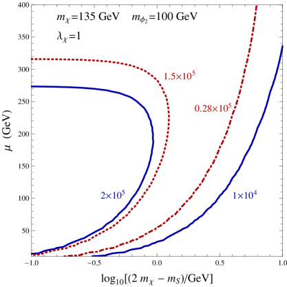
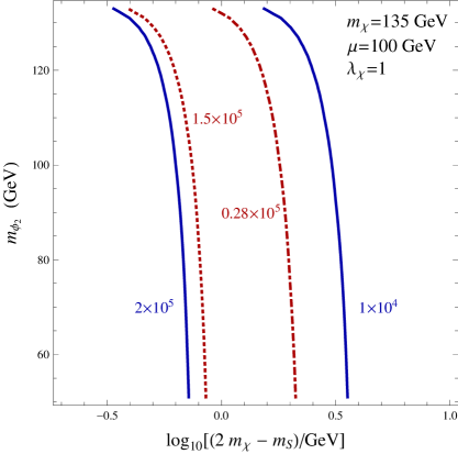
Figure 3: Left panel: the contour plots of the annihilation rates in pb$\cdot$c for $\mu$ and the mass difference $(2m_{\chi}-m_{S})$. The red and dotted line is the required cross section to explain the INTEGRAL data for the Einasto profile, while the red and dotdashed line is for the NFW profile in Eq. (4). Right panel: the same as the left one but in terms of $m_{\phi_{2}}$ and $(2m_{\chi}-m_{S})$.

For INTEGRAL, we need to calculate the velocity-averaged annihilation rate, which is given by

$$\langle\sigma v_{r}\rangle_{511}=\left\langle(\sigma v_{r})_{\phi_{2}\phi_{2}}(v_{r})\right\rangle=\frac{x^{3/2}}{\sqrt{4\pi}}\int v_{r}^{2}dv_{r}e^{-xv_{r}^{2}/4}(\sigma v_{r})_{\phi_{2}\phi_{2}}(v_{r})\,,$$ (13)

where $x=m_{\chi}/T=v_{0}^{-2}$ with $v_{0}$ determining the variance of the Gaussian dark matter velocity distribution. In our numerical calculation, we neglect the upper limit of the integration, which is controlled by the escaping velocity of dark matter in the galaxy and has only a small effect on our final results.

In Fig. 3, we show the contours of the annihilation rates of $\langle\sigma v_{r}\rangle_{511}$ in terms of $\mu$ and $(2m_{\chi}-m_{S})$ in the left panel, also $m_{\phi_{2}}$ and $(2m_{\chi}-m_{S})$ in the right panel. To obtain a large annihilation rate around $10^{5}$ pb to explain the INTEGRAL data, the resonance mass has to be very close to twice of the dark matter mass. The mass splitting should be a few GeV for the parameter $\mu\sim 100$ GeV. In Fig. 3, we only presented the results for $m_{S}\lesssim 2m_{\chi}$. The case with $m_{S}\gtrsim 2m_{\chi}$ has an additional contribution to the total width of $S$ from $S\rightarrow\chi\bar{\chi}$, and has similar results. From the right panel of Fig. 3, we can see that the annihilation rate is insensitive to $m_{\phi_{2}}$ except for the region with $m_{\phi_{2}}\sim m_{\chi}$. One might think that $\phi_{2}$ can be as light as possible. However, a light $\phi_{2}$ generated from dark matter annihilation can have a large Lorentz boost. As a consequence, $e^{+}$ from $\phi_{2}$ decays is also boosted and too energetic to explain the INTEGRAL data [12]. Therefore, we restrict the parameter space in our later study to have $m_{\phi_{2}}$ at least above 50 GeV.

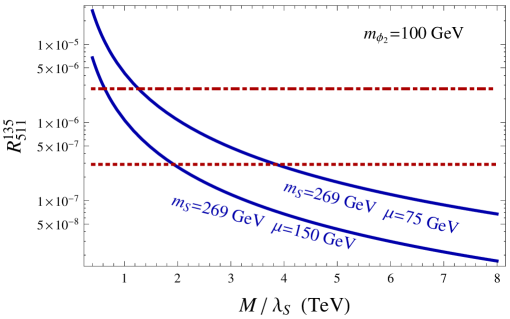
Figure 4: The ratio of annihilation rates for the Fermi-LAT and INTEGRAL signals as a function of the cutoff of the higher-dimensional operators. Here, we choose $m_{\phi_{2}}=100$ GeV. The dotted and dot-dashed lines (red) indicate the approximate value from experimental measurements for two different dark matter profiles.

For the Fermi-LAT signal, instead of obtaining the absolute annihilation rate, we calculate the ratio of the required signal strengths for Fermi-LAT and INTEGRAL. The ratio is equal to the branching ratio of the two decay channels of $S$ in Eq. (12), assuming that the additional contribution from the process $\phi_{1}\phi_{1}\rightarrow\gamma\gamma$ is small. By taking the ratio, the dependence on the resonance propagator is cancelled and we have

$$R^{135}_{511}=\frac{\lambda_{S}^{2}\,\alpha^{2}\,m_{S}^{4}}{2\,\pi^{2}\,M^{2}\,\mu^{2}}\,\left(1\,-\,\frac{4m_{\phi_{2}}^{2}}{m_{S}^{2}}\right)^{-1/2}\,.$$ (14)

We show this ratio of the annihilation rates in Fig. 4 by fixing $m_{\phi_{2}}=100$ GeV. From Fig. 4, we can find that the cutoff of the operators in Eq. (7) should be several TeV.

From the effective operator analysis in this section, we have seen that it is possible to explain the required annihilation rates for both INTEGRAL and Fermi-LAT. Our model is economical in a sense that only a few operators and a small number of degrees of freedom are required to explain the data. On the other hand, we should also admit that the resonance requirement of $(2m_{\chi}-m_{S})\ll m_{S}$ is a tuning point of the parameter space of the current model. Additional ingredients are therefore required to explain this delicate mass relation. We leave this direction of exploration to a future study. Here we emphasize that the ratio of INTEGRAL and Fermi-LAT signals are independent on the way we enhance the annihilation cross sections. Thus one can attach the rest of the model to any other ways of enhancement, e.g. a light mediator in the $t$-channel plus the Sommerfeld enhancement [48]. In the next section, we construct a renormalizable model to UV complete the Lagrangian in Eq. (7) and explain the common origin of the last two operators in Eq. (7).

3.2 Renormalizable model

One way to UV complete the effective Lagrangian in the previous section is to introduce electromagnetic charged states to connect the dark matter sector to photon. In order to have the state $\phi_{1}$ stable, at least two charged particles are required to preserve the discrete symmetry associated with $\phi_{1}$. As one example, we introduce two charged complex scalar fields, $X_{1}$ and $X_{2}$. One could also study fermionic charged states in the same procedure. Under $U(1)_{Y}$ or $U(1)_{em}$ after electroweak symmetry breaking, $X_{1}$ and $X_{2}$ have charge one. The global symmetries that we introduce contain a ${\cal Z}_{2}$ symmetry responsible for the stability of the dark matter particles and a $U(1)_{\phi}$ protecting the mass degeneracy of $\phi_{1}$ and $\phi_{2}$. We show the field content and symmetries in Table 1.

spin $U(1)_{Y}$ $U(1)_{\phi}$ $\mathbb{Z}_{2}$ $\chi$ $\frac{1}{2}$ 0 0 $-$ $S$ 0 0 0 $+$ $\Phi=\frac{1}{\sqrt{2}}(\phi_{1}+i\phi_{2})$ 0 0 1 $-$ $X_{1}$ 0 1 1 $-$ $X_{2}$ 0 1 0 $+$

Table 1: Matter content and corresponding charge assignments. The global symmetry $U(1)_{\phi}$ is only an approximate one. The small mass splitting of $\phi_{1}$ and $\phi_{2}$ breaks it.

Based on the symmetries in Table 1, we have the following subset of operators allowed by the symmetries,

$$-{\cal L} \supset i\,\lambda_{\chi}\,\overline{\chi}\gamma^{5}\chi\,S+\mu\,S\,\Phi^{\dagger}\Phi\,+\,\mu_{1}(\Phi X_{1}X_{2}^{\dagger}+\Phi^{\dagger}X_{1}^{\dagger}X_{2})\,+\,\mu_{2}\,S\,X_{1}X_{1}^{\dagger}\,+\,\mu_{3}\,S\,X_{2}X_{2}^{\dagger}\,+\lambda_{1}\,\Phi\Phi^{\dagger}HH^{\dagger}$$ (15)

$$\,+\,\frac{1}{2}m_{S}^{2}\,S^{2}\,+\,m_{\phi}^{2}\Phi\Phi^{\dagger}\,+\,\frac{1}{2}m_{\phi}\,\delta\,(\Phi^{2}+\Phi^{\dagger\,2})\,+\,m_{X_{1}}^{2}X_{1}X_{1}^{\dagger}\,+\,m_{X_{2}}^{2}X_{2}X_{2}^{\dagger}$$

$$\,+\,\lambda^{i}_{e}\,X_{1}\,\overline{\chi}\,e_{R}^{i}+h.c.\,.$$

Here we only list the operators which are relevant to the processes we concern in this paper. Especially the operator $SHH^{\dagger}$ is neglected, which is assumed to have a small coefficient. The last operator generically introduces lepton flavor violation processes, so the couplings $\lambda^{i}_{e}$ ($i$ is the flavor index) should be small.

We first note that the vertices $(\Phi X_{1}X_{2}^{\dagger}+\Phi^{\dagger}X_{1}^{\dagger}X_{2})$ could generate the charge radius operator for the $\Phi$ field as shown in the last operator in Eq. (7). After a calculation of the triangle diagram with $X_{1}$ and $X_{2}$ propagating in the loop, we get the Feynman rule of the following operator $\partial_{\mu}\Phi\partial_{\nu}\Phi^{\dagger}F^{\mu\nu}=i\,\partial_{\mu}\phi_{2}\partial_{\nu}\phi_{1}F^{\mu\nu}$

$$\frac{e\,\mu_{1}^{2}}{32\,\pi^{2}}\int^{1}_{0}dx\int^{1-x}_{0}dy\left[\frac{(1-2x)\,k_{1}^{\alpha}+(1-2y)\,k_{2}^{\alpha}}{(1-x-y)m_{X_{2}}^{2}+(x+y)\,m_{X_{1}}^{2}+(x\,k_{1}+y\,k_{2})^{2}-x\,k_{1}^{2}-y\,k_{2}^{2}}-(m_{X_{1}}\leftrightarrow m_{X_{2}})\right]\,,$$ (16)

where $k_{1}$ and $k_{2}$ are momenta of $\phi_{1}$ and $\phi_{2}$ with opposite directions towards the vertex. In the limit $m^{2}_{X_{1,2}}\gg k_{1}^{2},k_{2}^{2}$, we can match to the coefficient of the effective operator in Eq. (7) as

$$\frac{\lambda_{\Phi}}{M^{2}} = \,\frac{\mu_{1}^{2}\left[3(m_{X_{1}}^{4}-m_{X_{2}}^{4})-2(m_{X_{1}}^{4}+4m_{X_{1}}^{2}m_{X_{2}}^{2}+m_{X_{2}}^{4})\log{(m_{X_{1}}/m_{X_{2}})}\right]}{6(m_{X_{1}}^{2}-m_{X_{2}}^{2})^{4}}\,.$$ (17)

We notice that the above formula vanishes when $m_{X_{1}}=m_{X_{2}}$. This can be understood by the enhanced discrete symmetry, $\Phi\rightarrow\Phi^{\dagger},X_{1}\leftrightarrow X_{2}$, in the Lagrangian when $X_{1}$ and $X_{2}$ have degenerate masses. The charge-radius operator violates this discrete symmetry, thus cannot be generated when $m_{X_{1}}=m_{X_{2}}$. Another more intuitive explanation is to think $\Phi$ as a composite particle of $X_{1}^{+}$ and $X_{2}^{-}$. If the mass of $X_{2}^{-}$ is much heavier than $X_{1}^{+}$, one can treat $X_{1}^{+}$ as a particle rotating around $X_{2}^{-}$ and have a nonzero charge radius. However, for the mass degenerate case, $X_{1}^{+}$ and $X_{2}^{-}$ should be treated with equal foot and rotate around the center with the same radius. As a result, for each orbit the net charge is zero and the charge radius is zero.

Similarly, we can integrate out $X_{1}$ and $X_{2}$ to generate the effective operator coupling $S$ to two photons. To match the coefficient in Eq. (7), we have

$$\frac{\lambda_{S}}{M} = \frac{1}{12}\left(\frac{\mu_{2}}{m_{X_{1}}^{2}}+\frac{\mu_{3}}{m_{X_{2}}^{2}}\right)\,.$$ (18)

In the limit $m^{2}_{X_{2}}/\mu_{3}\ll m^{2}_{X_{1}}/\mu_{2}$, we have

$$m_{X_{2}}\approx 410~{}\mbox{GeV}\times\left(\frac{M/\lambda_{S}}{2~{}\mbox{TeV}}\right)^{1/2}\,\left(\frac{\mu_{3}}{1~{}\mbox{TeV}}\right)^{1/2}\,.$$ (19)

Using the values of $M/\lambda_{S}$ in Fig. 4, we anticipate at least the charged particle $X_{2}$ to have a mass below 1 TeV. This charged particle $X_{2}$ can decay into one lepton plus one neutrino, for example via the higher dimensional operator $X_{2}\tilde{H}\bar{L}\,e_{R}$.

3.3 Dark Matter Relic Abundance

In our DeDM model, we have two stable particles in our spectrum: $\chi$ and $\phi_{1}$. In our previous analysis, we have assumed that the majority of dark matter in our universe is mainly composed of $\chi$. To justify our assumption, it is important to study the thermal history of $\chi$ and $\phi_{1}$. In this section, we demonstrate that our setup contains enough ingredients to induce a right relic abundance for $\chi$, thus it could be the dominant part of the dark matter in our current Universe.

The thermal relic abundance of $\phi_{1}$ is controlled by the parameter $\lambda_{1}$ in Eq. (15), which is similar to the “Higgs portal” dark matter models [49, 50]. For $m_{\phi_{1}}<m_{h}$, the main annihilation cross section is [51]

$$\sigma v_{r}(\phi_{1}) = \frac{2\,\lambda_{1}^{2}\,v_{\rm EW}^{2}}{(4\,m_{\phi_{1}}^{2}-m_{h}^{2})^{2}+m_{h}^{2}\,\Gamma_{h}^{2}(m_{h})}\,\frac{\Gamma_{h}(2m_{\phi_{1}})}{2\,m_{\phi_{1}}}\,,$$ (20)

where $v_{\rm EW}=246$ GeV is the electroweak vacuum expectation value. The function $\Gamma_{h}(m)$ is the width of a Higgs boson in the SM with a mass at $m$. For $\lambda_{1}=1$, $m_{\phi_{1}}=100$ GeV and $m_{h}=125$ GeV, we have $\sigma v_{r}(\phi_{1})\approx 581$ pb and $\Omega_{\phi_{1}}h^{2}\approx 1.4\times 10^{-3}\times\Omega_{\rm DM}h^{2}$. Thus the relic abundance of $\phi_{1}$ can be naturally small.

To satisfy the dark matter relic abundance, a non-trivial thermal history of $\chi$ is needed. This is because a large annihilation cross section in Eq. (10) is needed to explain the INTEGRAL data. The thermal relic abundance of $\chi$ is very small compared to the required dark matter energy density. Noticing that the last operator in Eq. (15) can introduce the decay channel, $X_{1}^{+}\rightarrow\chi\,e^{+}$, the late decay of thermally abundant $X^{+}_{1}$ particles can generate enough $\chi$, and therefore explain why $\chi$ could be the majority of dark matter.

We first calculate the thermal relic abundance of the charged particle $X^{\pm}_{1}$ before it decays into $\chi$ and a positron/electron. There are two classes of annihilation channels for $X^{\pm}_{1}$. The first class has a photon or $Z$ boson exchanging in the $s$-channel with final states as a pair of the SM fermions, $W^{+}\,W^{-}$ gauge bosons, and $h\,Z$. The second class includes the $t$-channel diagrams, interfering with seagull diagrams. Assuming that the mass $X_{1}^{\pm}$ is far above the SM particle masses and neglecting the SM particle masses, we have

$$\sigma v_{r}(X_{1}^{+}X_{1}^{-}\rightarrow\gamma\,\gamma) = \frac{e^{4}}{8\,\pi\,m_{X_{1}}^{2}}\,,\qquad\sigma v_{r}(X_{1}^{+}X_{1}^{-}\rightarrow Z\,Z)=\frac{e^{4}\,s_{W}^{4}}{8\,\pi\,c_{W}^{4}\,m_{X_{1}}^{2}}\,,\;$$ (21)

$$\sigma v_{r}(X_{1}^{+}X_{1}^{-}\rightarrow\gamma\,Z) = \frac{3\,e^{4}\,s_{W}^{2}}{4\,\pi\,c_{W}^{2}\,m_{X_{1}}^{2}}\,,\qquad\sigma v_{r}(X_{1}^{+}X_{1}^{-}\rightarrow h\,Z)=\frac{e^{4}}{1536\,\pi\,c_{W}^{4}\,m_{X_{1}}^{2}}\,v_{r}^{2}\,,$$ (22)

$$\sigma v_{r}(X_{1}^{+}X_{1}^{-}\rightarrow W^{+}W^{-}) = \frac{e^{4}}{1536\,\pi\,c_{W}^{4}\,m_{X_{1}}^{2}}\,v_{r}^{2}\,,\;$$ (23)

$$\sigma v_{r}(X_{1}^{+}X_{1}^{-}\rightarrow\bar{f}f) = \frac{e^{4}\,n^{f}_{c}\,\left[c_{W}^{2}-2c_{W}s_{W}\,q^{f}\,g_{V}^{f}+s_{W}^{2}(g_{A}^{f\,2}\,+\,g_{V}^{f\,2})\right]}{96\,\pi\,c_{W}^{2}\,m_{X_{1}}^{2}}\,v_{r}^{2}\,,$$ (24)

Here, $q^{f}$ is the electric charge of the SM fermion; $g_{A}^{f}\,(g_{V}^{f})$ is the axi-vector (vector) couplings of the $Z$ to the SM fermion up to the electric coupling $e$; $n^{f}_{c}=3$ for quarks and 1 for leptons. To derive the above formulas, we have only included the leading terms in $v_{r}$ for each equation. If the charged particle could occupy the total energy of dark matter in our universe, $\Omega_{\rm DM}h^{2}=0.11$, the required mass is calculated to be $m_{X_{1}}\approx 750$ GeV. To derive this mass, we have found that the $p$-wave suppressed annihilation cross section or the terms at ${\cal O}(v_{r}^{2})$ is subdominant compared to the total annihilation cross section.

For a lifetime of $X_{1}^{\pm}$ not too long in the cosmological time scale, we should anticipate that $X_{1}^{+}$ has already decayed into its daughter particle and the final dark matter in our current universe is composed of $\chi$. On the other hand, the lifetime of $X_{1}^{\pm}$ can not be too short. Otherwise, the produced $\chi$ particles from $X_{1}^{\pm}$ decays in the early universe can easily annihilate away and do not provide enough dark matter energy density. To calculate the thermal history of the $\chi$ field, one needs to solve for the following coupled Boltzmann equations between $\chi$ and $X_{1}^{\pm}$

$$\frac{dn_{X_{1}}}{dt}\,+\,3\,H\,n_{X_{1}} = -\langle\sigma v\rangle_{X_{1}}\left(n_{X_{1}}^{2}-n_{X_{1}}^{{\rm eq}\,2}\right)\,-\,n_{X_{1}}\,\Gamma_{X_{1}}\,,$$ (25)

$$\frac{dn_{\chi}}{dt}\,+\,3\,H\,n_{\chi} = \,-\,\langle\sigma v\rangle_{\chi}\left(n_{\chi}^{2}-n_{\chi}^{{\rm eq}\,2}\right)\,+\,n_{X_{1}}\,\Gamma_{X_{1}}\,.$$ (26)

Here, in the radiation dominated era, $H=(8\pi\rho/3M_{\rm Pl})^{1/2}$, $t=1/(2H)$, $\rho(T)=g_{*}\,\pi^{2}\,T^{4}/30$, and $n^{{\rm eq}}_{i}(T)=g_{i}(m_{i}T/2\pi)^{3/2}e^{-m_{i}/T}$, where $g_{*}=86.25$ is the number of degrees of relativistic freedom and $g_{\chi}=4$ and $g_{X_{1}}=2$. It is convenient to rescale the number density by the entropy and to define the quantity $Y_{i}\equiv n_{i}/s$ with $s=2\pi^{2}g_{*}T^{3}/45$. The coupled equations become

$$\frac{dY_{X_{1}}}{dx} = -\frac{s\,\langle\sigma v\rangle_{X_{1}}}{Hx}\,\left(Y_{X_{1}}^{2}-Y_{X_{1}}^{{\rm eq}\,2}\right)\,-\,\frac{\Gamma_{X_{1}}Y_{X_{1}}}{Hx}\,,$$ (27)

$$\frac{dY_{\chi}}{dx} = \,-\,\frac{s\,\langle\sigma v\rangle_{\chi}}{Hx}\left(Y_{\chi}^{2}-Y_{\chi}^{{\rm eq}\,2}\right)\,+\,\frac{\Gamma_{X_{1}}Y_{X_{1}}}{Hx}\,,$$ (28)

where $x\equiv m_{\chi}/T$ and $dx/dt=Hx$. The final $\chi$ relic abundance is given by $\Omega_{\chi}=\rho_{\chi}/\rho_{c}$, where $\rho_{c}=3H_{0}^{2}M^{2}_{\rm Pl}/8\pi=1.0539\times 10^{-5}h^{2}~{}\mbox{GeV\,cm}^{-3}$ is the critical density corresponding to a flat universe and $\rho_{\chi}=m_{\chi}s_{0}Y_{\chi}({\infty})$ with $s_{0}=2889.2\,\mbox{cm}^{-3}$ being the entropy today.

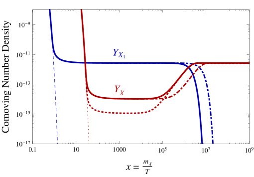
Figure 5: The comoving number density as a function of the temperature. Here, we choose $m_{\chi}=135$ GeV and $m_{X_{1}}=3.8$ TeV. The annihilation cross section of $X_{1}$, approximately 0.03 pb, is determined by its interactions with electroweak gauge bosons. The solid lines are for $\langle\sigma v_{r}\rangle_{\chi}=10$ pb and $\tau_{X_{1}}=10$ s; the dotdashed lines are for $\langle\sigma v_{r}\rangle_{\chi}=10$ pb and $\tau_{X_{1}}=100$ s; the dotted and red line is for $\langle\sigma v_{r}\rangle_{\chi}=100$ pb and $\tau_{X_{1}}=10$ s. The relic abundance of $\chi$ satisfies the observed dark matter energy density, $\Omega_{\chi}h^{2}=0.11$.

At the temperature region with ${\cal O}(20)<x<1000$, the decaying terms in Eq. (27) and (28) are not important. The number densities of $X_{1}$ and $\chi$ reach their separate freeze-out values. Since the cross section of $\chi$ is much larger than $X_{1}$, the freeze-out number density for $\chi$ is much below the one of $X_{1}$. At a later time, only the last terms in Eq. (27) and (28) become important. One can easily show that the quantity $Y_{X_{1}}+Y_{\chi}$ is a conserved number. As a result, the final number density of $\chi$ should just match to the number density of $X_{1}$ at ${\cal O}(20)$. So, approximately we have the relic abundance of $\chi$ as

$$\Omega_{\chi}h^{2}\approx 0.11\times\frac{m_{\chi}}{135~{}\mbox{GeV}}\,\times\frac{m_{X_{1}}}{3.8~{}\mbox{TeV}}\,,$$ (29)

So, the charged particle $X_{1}$ is predicted to be 3.8 TeV and the other charged particle $X_{2}$ should be below around 1 TeV to explain the ratio of INTEGRAL and Fermi-LAT cross sections in Eq. (18).

We solve the coupled equations in Eq. (28) numerically and show both comoving number densities of $\chi$ and $X_{1}$ in Fig. 5. We find that if the mass of $X_{1}$ is 3.8 TeV, it generates the relic abundance for $\chi$ which satisfies the total dark matter energy density, $\Omega_{\chi}h^{2}=0.11$. In the blue solid and the red solid lines, for $\langle\sigma v_{r}\rangle_{\chi}=10$ pb  and $\tau_{X_{1}}=10$ s we show the evolutions of the $X_{1}$ and $\chi$ comoving number densities as a function of temperature. As can be seen from Fig. 5 and at $x\approx 20$, both $X_{1}$ and $\chi$ have reached ordinary relic abundances according to their respective annihilation cross sections. At $x\approx 10^{5}-10^{6}$, $X_{1}$ starts to decay and its number density drops rapidly. Meanwhile, the stable $\chi$ particle number density increases and reaches a plateau at around $10^{7}$. The final number density of the $\chi$ field is found to be independent on the lifetime $\tau_{X_{1}}$, as long as the decay happens late enough so that the annihilation of $\chi$ is not important any more. The actual time for $\chi$ to reach its eventual number density is proportional to $\sqrt{\tau_{X_{1}}}$.

To satisfy the dark matter relic abundance, the lifetime of the charged particle $X_{1}$ can be $\leq 100\,s$ . For such a late decayed particle, we need to worry about its modification on the Big Bang nucleosynthesis (BBN) history. Since the main decaying product of $X_{1}$ is into leptons plus the stable $\chi$, the BBN constrains are fairly weak. From Ref. [52], the ${}^{6}\mbox{Li}/^{7}\mbox{Li}$ ratio constrains the lifetime of $X_{1}$ to be $\tau_{X_{1}}<10^{5}\,s$ for $\Omega_{X_{1}}h^{2}\approx 0.1$ if it would have not decayed. As pointed in Ref. [53, 54], the long-lived charged particle, with a lifetime $\tau_{X_{1}}>10^{3}\,s$, can form a bound state with nuclei and enhance the ⁶Li production. The parameter space in our model can indeed satisfy the BBN constraints.

4 Discussion and conclusions

The charged particle $X_{1}$ in our model behaves as a heavy stable charged particle (HSCP) at colliders. The current searches from CMS at $\sqrt{s}=7$ TeV and 5.0 fb^-1 have set a lower limit on the mass of $X_{1}$ to be 223 GeV at 95% C.L. [55]. For the predicted mass of $X_{1}$ around 3.8 TeV, the existing studies have shown that the 14 TeV LHC with 100 fb^-1 can reach the HSCP up to a mass around 1 TeV. So, unlikely the stable charged particle can be discovered at the 14 TeV LHC. However, for the other charged particle $X_{2}$ its mass should be below 1 TeV and could be a long-lived particle or decay into SM particles, for instance $X_{2}^{+}\rightarrow e^{+}\nu_{e}$. The parameter space of the $X_{2}$ particle will be well explored at the LHC 14 TeV running.

One feature of our model is directly using photon as a mediator to link the dark matter sector to positron/electron. Unfortunately, other than searching for the charged particles responsible for the charge radius operator, in the near future there is no additional observable dark matter direct or indirect signatures for the $\chi$ field, which has interactions with SM particles suppressed by the TeV scale cutoff of the effective operators. The minor component of dark matter, $\phi_{1}$, may have detectable effects. However, that highly relies on the parameters one chooses, thus we do not pursue that in detail here. Another ingredient that we utilize is the $s$-channel resonance particle to increase the annihilation cross section. We want to stress that this option is not a unique one and is introduced just for convenience. One can also introduce a light mediator in the $t$-channel plus the Sommerfeld enhancement to achieve the same goal [48].

In summary, we have constructed a realistic model to have the same dark matter particle responsible for both the INTEGRAL 511 keV and Fermi-LAT 135 GeV lines. Through an $s$-channel resonance, the dark matter particles annihilate into a complex scalar, which couples to photon via a charge-radius operator. For a few MeV mass splitting between the real and imaginary parts of the complex scalar, two pairs of electron and positron are the main visible particles from dark matter annihilation. We have worked out the parameter space and have found that both the large cross section required for INTEGRAL and the small cross section for Fermi-LAT can be simultaneously accommodated in our model. The thermal relic abundance of dark matter is achieved by the late decay of a charged particle, which also generates the charge-radius operator. The other charged particle responsible for the charge-radius operator is predicted to have a mass below 1 TeV. The 14 TeV LHC will concretely test the scenario presented in this paper.

Acknowledgments

We would like to thank James Cline, Tim Cohen, Douglas Finkbeiner, JoAnne Hewett, Dan Hooper, Jessie Shelton, Tracy Slatyer, Aaron Vincent and Jay Wacker for useful discussions and comments. YB is supported by start-up funds from the University of Wisconsin, Madison. YB thanks SLAC for their warm hospitality. SLAC is operated by Stanford University for the US Department of Energy under contract DE-AC02-76SF00515. We also thank the Aspen Center for Physics, under NSF Grant No. 1066293, where part of this work was completed. Support for the work of M.S. was provided by NASA through Einstein Postdoctoral Fellowship grant number PF2-130102 awarded by the Chandra X-ray Center, which is operated by the Smithsonian Astrophysical Observatory for NASA under contract NAS8-03060.

References

- [1] L. Bergstrom and P. Ullio, Full one loop calculation of neutralino annihilation into two photons, Nucl.Phys. B504 (1997) 27–44, [hep-ph/9706232].
- [2] Z. Bern, P. Gondolo, and M. Perelstein, Neutralino annihilation into two photons, Phys.Lett. B411 (1997) 86–96, [hep-ph/9706538].
- [3] L. Bergstrom, P. Ullio, and J. H. Buckley, Observability of gamma-rays from dark matter neutralino annihilations in the Milky Way halo, Astropart.Phys. 9 (1998) 137–162, [astro-ph/9712318].
- [4] P. Ullio and L. Bergstrom, Neutralino annihilation into a photon and a Z boson, Phys.Rev. D57 (1998) 1962–1971, [hep-ph/9707333].
- [5] M. Perelstein and A. Spray, Indirect Detection of Little Higgs Dark Matter, Phys.Rev. D75 (2007) 083519, [hep-ph/0610357].
- [6] G. Bertone, C. Jackson, G. Shaughnessy, T. M. Tait, and A. Vallinotto, Gamma Ray Lines from a Universal Extra Dimension, JCAP 1203 (2012) 020, [arXiv:1009.5107].
- [7] W. N. Johnson, III, F. R. Harnden, Jr., and R. C. Haymes, The Spectrum of Low-Energy Gamma Radiation from the Galactic-Center Region., Astrophys. J. Lett. 172 (Feb., 1972) L1.
- [8] W. N. Johnson, III and R. C. Haymes, Detection of a Gamma-Ray Spectral Line from the Galactic-Center Region, Astrophys. J. 184 (Aug., 1973) 103–126.
- [9] R. C. Haymes, G. D. Walraven, C. A. Meegan, R. D. Hall, F. T. Djuth, and D. H. Shelton, Detection of nuclear gamma rays from the galactic center region, Astrophys. J. 201 (Nov., 1975) 593–602.
- [10] M. Leventhal, C. J. MacCallum, and P. D. Stang, Detection of 511 keV positron annihilation radiation from the galactic center direction, Astrophys. J. Lett. 225 (Oct., 1978) L11–L14.
- [11] R. W. Bussard, R. Ramaty, and R. J. Drachman, The annihilation of galactic positrons, Astrophys. J. 228 (Mar., 1979) 928–934.
- [12] Y. Ascasibar, P. Jean, C. Boehm, and J. Knoedlseder, Constraints on dark matter and the shape of the Milky Way dark halo from the 511-keV line, Mon.Not.Roy.Astron.Soc. 368 (2006) 1695–1705, [astro-ph/0507142].
- [13] E. Churazov, R. Sunyaev, S. Sazonov, M. Revnivtsev, and D. Varshalovich, Positron annihilation spectrum from the Galactic Center region observed by SPI/INTEGRAL, Mon.Not.Roy.Astron.Soc. 357 (2005) 1377–1386, [astro-ph/0411351].
- [14] G. Weidenspointner, C. Shrader, J. Knoedlseder, P. Jean, V. Lonjou, et. al., The sky distribution of positronium annihilation continuum emission measured with spi/integral, Astron.Astrophys. (2006) [astro-ph/0601673].
- [15] J. F. Beacom and H. Yuksel, Stringent constraint on galactic positron production, Phys.Rev.Lett. 97 (2006) 071102, [astro-ph/0512411].
- [16] N. Prantzos, C. Boehm, A. M. Bykov, R. Diehl, K. Ferriere, N. Guessoum, P. Jean and J. Knoedlseder et al., arXiv:1009.4620 [astro-ph.HE].
- [17] C. Picciotto and M. Pospelov, Unstable relics as a source of galactic positrons, Phys.Lett. B605 (2005) 15–25, [hep-ph/0402178].
- [18] D. Hooper and L.-T. Wang, Possible evidence for axino dark matter in the galactic bulge, Phys.Rev. D70 (2004) 063506, [hep-ph/0402220].
- [19] C. Boehm, D. Hooper, J. Silk, M. Casse, and J. Paul, MeV dark matter: Has it been detected?, Phys.Rev.Lett. 92 (2004) 101301, [astro-ph/0309686].
- [20] M. Pospelov, A. Ritz, and M. Voloshin, Secluded WIMP dark matter, Physics Letters B 662 (Apr., 2008) 53–61, [arXiv:0711.4866].
- [21] D. Hooper and K. M. Zurek, Natural supersymmetric model with MeV dark matter, Phys. Rev. D 77 (Apr., 2008) 087302, [arXiv:0801.3686].
- [22] J.-H. Huh, J. E. Kim, J.-C. Park, and S. C. Park, Galactic 511 keV line from MeV millicharged dark matter, Phys. Rev. D 77 (June, 2008) 123503, [arXiv:0711.3528].
- [23] M. Pospelov and A. Ritz, The galactic 511 keV line from electroweak scale WIMPs, Phys.Lett. B651 (2007) 208–215, [hep-ph/0703128].
- [24] D. P. Finkbeiner and N. Weiner, Exciting Dark Matter and the INTEGRAL/SPI 511 keV signal, Phys.Rev. D76 (2007) 083519, [astro-ph/0702587].
- [25] N. Arkani-Hamed, D. P. Finkbeiner, T. R. Slatyer, and N. Weiner, A theory of dark matter, Phys. Rev. D 79 (Jan., 2009) 015014, [arXiv:0810.0713].
- [26] F. Chen, J. M. Cline, and A. R. Frey, New twist on excited dark matter: Implications for INTEGRAL, PAMELA/ATIC/PPB-BETS, DAMA, Phys. Rev. D 79 (Mar., 2009) 063530, [arXiv:0901.4327].
- [27] F. Chen, J. M. Cline, A. Fradette, A. R. Frey, and C. Rabideau, Exciting dark matter in the galactic center, Phys.Rev. D81 (2010) 043523, [arXiv:0911.2222].
- [28] R. Morris and N. Weiner, Low Energy INTEGRAL Positrons from eXciting Dark Matter, arXiv:1109.3747.
- [29] C. Weniger, A Tentative Gamma-Ray Line from Dark Matter Annihilation at the Fermi Large Area Telescope, arXiv:1204.2797.
- [30] T. Bringmann, X. Huang, A. Ibarra, S. Vogl, and C. Weniger, Fermi LAT Search for Internal Bremsstrahlung Signatures from Dark Matter Annihilation, arXiv:1203.1312.
- [31] M. Su and D. P. Finkbeiner, Strong Evidence for Gamma-ray Line Emission from the Inner Galaxy, arXiv:1206.1616.
- [32] F.-L. Collaboration, Search for GammSearch Gamma-ray Spectral Lines in the Milky Way Diffuse with the Fermi Large Area Telescope, .
- [33] T. Bringmann and C. Weniger, Gamma Ray Signals from Dark Matter: Concepts, Status and Prospects, arXiv:1208.5481.
- [34] W. Buchmuller and M. Garny, Decaying vs Annihilating Dark Matter in Light of a Tentative Gamma-Ray Line, JCAP 1208 (2012) 035, [arXiv:1206.7056].
- [35] L. Bouchet, J.-P. Roques, and E. Jourdain, On the morphology of the electron-positron annihilation emission as seen by SPI/INTEGRAL, Astrophys.J. 720 (2010) 1772–1780, [arXiv:1007.4753].
- [36] M. Su and D. P. Finkbeiner, Double Gamma-ray Lines from Unassociated Fermi-LAT Sources, ArXiv e-prints (July, 2012) [arXiv:1207.7060].
- [37] G. Jungman, M. Kamionkowski, and K. Griest, Supersymmetric dark matter, Phys.Rept. 267 (1996) 195–373, [hep-ph/9506380].
- [38] P. Jean, J. Knodlseder, W. Gillard, N. Guessoum, K. Ferriere, et. al., Spectral analysis of the galactic e+ e- annihilation emission, Astron.Astrophys. 445 (2006) 579–589, [astro-ph/0509298].
- [39] J. F. Navarro, E. Hayashi, C. Power, A. Jenkins, C. S. Frenk, et. al., The Inner structure of Lambda-CDM halos 3: Universality and asymptotic slopes, Mon.Not.Roy.Astron.Soc. 349 (2004) 1039, [astro-ph/0311231].
- [40] J. F. Navarro, C. S. Frenk, and S. D. White, A Universal density profile from hierarchical clustering, Astrophys.J. 490 (1997) 493–508, [astro-ph/9611107].
- [41] A. C. Vincent, P. Martin, and J. M. Cline, Interacting dark matter contribution to the Galactic 511 keV gamma ray emission: constraining the morphology with INTEGRAL/SPI observations, JCAP 1204 (2012) 022, [arXiv:1201.0997].
- [42] M. Ibe, H. Murayama, and T. Yanagida, Breit-Wigner Enhancement of Dark Matter Annihilation, Phys.Rev. D79 (2009) 095009, [arXiv:0812.0072].
- [43] H. M. Lee, M. Park, and W.-I. Park, Fermi Gamma Ray Line at 130 GeV from Axion-Mediated Dark Matter, ArXiv e-prints (May, 2012) [arXiv:1205.4675].
- [44] M. R. Buckley and D. Hooper, Implications of a 130 GeV Gamma-Ray Line for Dark Matter, ArXiv e-prints (May, 2012) [arXiv:1205.6811].
- [45] H. M. Lee, M. Park, and W.-I. Park, Axion-mediated dark matter and Higgs diphoton signal, arXiv:1209.1955.
- [46] Y. Bai and J. Shelton, Gamma Lines without a Continuum: Thermal Models for the Fermi-LAT 130 GeV Gamma Line, arXiv:1208.4100.
- [47] G. Chalons, M. J. Dolan, and C. McCabe, Neutralino dark matter and the Fermi gamma-ray lines, arXiv:1211.5154.
- [48] N. Arkani-Hamed, D. P. Finkbeiner, T. R. Slatyer, and N. Weiner, A Theory of Dark Matter, Phys.Rev. D79 (2009) 015014, [arXiv:0810.0713].
- [49] R. E. Shrock and M. Suzuki, INVISIBLE DECAYS OF HIGGS BOSONS, Phys.Lett. B110 (1982) 250.
- [50] V. Barger, P. Langacker, M. McCaskey, M. J. Ramsey-Musolf, and G. Shaughnessy, LHC Phenomenology of an Extended Standard Model with a Real Scalar Singlet, Phys.Rev. D77 (2008) 035005, [arXiv:0706.4311].
- [51] C. Burgess, M. Pospelov, and T. ter Veldhuis, The Minimal model of nonbaryonic dark matter: A Singlet scalar, Nucl.Phys. B619 (2001) 709–728, [hep-ph/0011335].
- [52] K. Jedamzik, Big bang nucleosynthesis constraints on hadronically and electromagnetically decaying relic neutral particles, Phys.Rev. D74 (2006) 103509, [hep-ph/0604251].
- [53] M. Pospelov, Particle physics catalysis of thermal Big Bang Nucleosynthesis, Phys.Rev.Lett. 98 (2007) 231301, [hep-ph/0605215].
- [54] K. Kohri and F. Takayama, Big bang nucleosynthesis with long lived charged massive particles, Phys.Rev. D76 (2007) 063507, [hep-ph/0605243].
- [55] CMS Collaboration, S. Chatrchyan et. al., Search for heavy long-lived charged particles in pp collisions at sqrt(s)=7 TeV, Phys.Lett. B713 (2012) 408–433, [arXiv:1205.0272].