Exploiting the shift of baryonic acoustic oscillations as a dynamical probe for dark interactions

Abstract

The baryonic acoustic peak in the correlation function of galaxies and galaxy clusters provides a standard ruler to probe the space-time geometry of the Universe, jointly constraining the angular diameter distance and the Hubble expansion rate. Moreover, non-linear effects can systematically shift the peak position, giving us the opportunity to exploit this clustering feature also as a dynamical probe. We investigate the possibility of detecting interactions in the dark sector through an accurate determination of the baryonic acoustic scale. Making use of the public halo catalogues extracted from the CoDECS simulations – the largest suite of N-body simulations of interacting dark energy models to date – we determine the position of the baryonic scale fitting a band-filtered correlation function, specifically designed to amplify the signal at the sound horizon. We analyze the shifts due to non-linear dynamics, redshift-space distortions and Gaussian redshift errors, in the range $0\leq z\leq 2$. Since the coupling between dark energy and dark matter affects in a particular way the clustering properties of haloes and, specifically, the amplitude and location of the baryonic acoustic oscillations, the cosmic evolution of the baryonic peak position might provide a direct way to discriminate interacting dark energy models from the standard $\Lambda$CDM framework. To maximize the efficiency of the baryonic peak as a dynamic probe, the correlation function has to be measured in redshift-space, where the baryonic acoustic shift due to non-linearities is amplified. The typical redshift errors of spectroscopic galaxy surveys do not significantly impact these results.

1 Introduction

Understanding the physical origin of the accelerated expansion of the Universe is one of the main drivers of the current cosmological research activity. The so-called $\Lambda$-Cold Dark Matter ($\Lambda$CDM) model is to date the most reliable cosmological scenario to explain such acceleration, due to its success in matching the observed properties of the large scale structure (LSS) of the Universe. However, there are still some observational tensions at small and intermediate scales, like the lack of luminous satellites in cold dark matter (CDM) haloes (see e.g. Navarro et al., 1996; Boylan-Kolchin et al., 2011), the observed low baryon fraction in galaxy clusters (see e.g. Ettori, 2003; McCarthy et al., 2007) and the high velocities detected in the large-scale bulk motion of galaxies (see e.g. Watkins et al., 2009) or in systems of colliding galaxy clusters, as the famous “Bullet Cluster” (see e.g. Lee & Komatsu, 2010). It is still unclear whether the above apparent disagreements are a consequence of some not well understood astrophysical phenomena at small scales, or if they really represent a signature of an underlying cosmological scenario different from the standard $\Lambda$CDM model. In any case, this provides an obvious motivation to explore alternative cosmological models that could explain these astrophysical anomalies. Furthermore, the nature of the dark sector of the Universe, made of dark energy (DE) – the component responsible for the late time acceleration – and dark matter (DM) – a kind of matter that negligibly interacts with radiation and can only be detected by its gravitational influence, is still unknown, even if it constitutes more than 95% of the total energy of the Universe.

In the last fifteen years, after the detection of the accelerated expansion of the Universe (Riess et al., 1998; Perlmutter et al., 1999; Schmidt et al., 1998), widespread theoretical and observational efforts have been made to clarify whether the observed DE component is just a cosmological constant $\Lambda$, or if its origin comes from other sources that can dynamically change in time. In this work, we investigate the LSS of the Universe in the so-called coupled (or interacting) DE models (cDE hereafter). This kind of cosmological scenarios are based on the dynamical evolution of a classical scalar field, $\phi$, that plays the role of the DE and interacts with the CDM particles by exchanging energy-momentum (see e.g. Wetterich, 1995; Amendola, 2000, 2004). Interestingly, cDE models can alleviate some observational tensions at small scales, that are presently not well understood in the $\Lambda$CDM cosmology, as mentioned above (see e.g. Baldi et al., 2010; Baldi & Pettorino, 2011; Lee & Baldi, 2011).

Baryonic Acoustic Oscillations (BAO) are the relic imprints left over by the primordial density perturbations in the early Universe, when the photon pressure was counteracting the gravitational collapse of baryons, generating acoustic waves in the baryon-photon plasma. When the Universe became cool enough to allow the electrons and protons to recombine, at $z\sim 1000$, baryons and photons decoupled and the acoustic waves became frozen in the baryon distribution. Baryons then progressively fell into CDM potential wells and CDM was, in turn, also attracted to baryon overdensities (see e.g. Peebles & Yu, 1970). The BAO feature, corresponding to the scale of the comoving “sound horizon”, can be detected in the matter distribution as a small excess in the number of galaxy pairs at $\sim$100 $h^{-1}\,\mbox{Mpc}$ , that creates either a single peak in the correlation function, $\xi(r)$, in configuration space, or a series of peaks in the power spectrum, $P(k)$, in Fourier space. As the sound horizon scale is well constrained by the cosmic microwave background (CMB) observations, the BAO location at different redshifts provides a standard ruler to measure the expansion history of the Universe and to constrain the DE equation of state, $w(z)$ (see e.g. Seo & Eisenstein, 2003; Albrecht et al., 2006; Amendola et al., 2012b). The BAO provide a powerful probe to investigate the nature of the late time acceleration, as they depend only slightly on the still uncertain astrophysical phenomena that could introduce systematic bias in the cosmological constraints.

Several independent measurements of the BAO feature in galaxy redshift surveys contributed to the great success of the concordance $\Lambda$CDM model (see e.g. Eisenstein et al., 2005; Cole et al., 2005; Hütsi, 2006; Percival et al., 2007; Padmanabhan et al., 2007; Okumura et al., 2008; Sánchez et al., 2009; Gaztañaga et al., 2009; Percival et al., 2010; Kazin et al., 2010; Blake et al., 2011; Beutler et al., 2011), and a number of future experiments are planned to use these features for precision cosmology, such as Euclid (Laureijs et al., 2011; Amendola et al., 2012b), BigBOSS (Schlegel et al., 2011), and the Wide-Field Infrared Survey Telescope (WFIRST).

In order to exploit the BAO as a robust standard ruler, all the systematic effects have to be kept under control and the position of the BAO peak has to be measured with high precision. The traditional estimators, $\xi(s)$ and $P(k)$, have some disadvantages that can affect the measure of the BAO at different redshifts. The former can be affected by the integral constraint at large-scale, if the cosmic number density of the population of mass tracers is not accurately known. The latter is instead affected by the uncertainty in the small-scale power, that is difficult to model due to non-linear effects. To reduce these possible systematics, Xu et al. (2010) proposed a new robust estimator to analyze LSS and BAO, band-filtering the information in the two-point correlation function. The above estimator has been recently used to extract cosmological constraints from the BAO feature in the WiggleZ data (Blake et al., 2011).

Non-linearities also affect the BAO as a standard ruler. According to linear perturbation theory, the sound horizon scale imprinted in the early Universe remains unaltered as a function of time. However, non-linearities cause a slight shift of the peak position relative to the linear prediction (see e.g. Seo & Eisenstein, 2005; Crocce & Scoccimarro, 2008; Angulo et al., 2008; Padmanabhan & White, 2009), and redshift-space distortions (RSD) further exacerbate this effect (see e.g. Smith et al., 2008). As a consequence, to calibrate the BAO as an unbiased standard ruler, the non-linear effects have to be accurately quantified in real- and redshift-space. Moreover, as we will discuss extensively in the next sections, the way that non-linearities and RSD affect the BAO feature depends on the assumed cosmological model. As a consequence, the BAO peak provides also a dynamical probe that could be of some help in discriminating between the $\Lambda$CDM model and alternative DE scenarios characterized by a different non-linear regime of structure evolution.

In this paper, we will focus our investigation on configuration space and extend to larger scales the work presented in Marulli et al. (2012a), analyzing the BAO feature in cDE models with the band-filtered correlation function of Xu et al. (2010). In particular, we focus on the shift of the BAO position due to non-linearities and RSD, in the redshift range $0\leq z\leq 2$. Moreover, we quantify the impact of Gaussian redshift errors on the BAO feature. To properly describe all the linear and non-linear effects at work, we employ a series of state-of-the-art N-body simulations for a wide range of different cDE scenarios – the COupled Dark Energy Cosmological Simulation project (CoDECS) (Baldi, 2012c) – that are used to investigate the impact that DE interactions can have on LSS, and in particular on BAO, with respect to the $\Lambda$CDM case.

The structure of the paper is as follows. In §2 and §3, we describe the cDE models and the exploited set of N-body experiments analyzed in this work to simulate the LSS in these cosmologies. In §4, we review our theoretical tools, describing the new statistic, $\omega_{0}(r_{s})$, used in our investigation. Our results are described in §5, where we analyze the CDM halo clustering at large scales, focusing on the shift of the BAO signal position through cosmic time. Finally, in §6 we draw our conclusions.

Table 1: List of cosmological models considered in the CoDECS project and their specific parameters (see text for details).

Model	Potential	$\alpha$	$\eta_{0}$	$\eta_{1}$	$w_{\phi}(z=0)$	$\sigma_{8}(z=0)$
$\Lambda$CDM	$V(\phi)=A$	–	–	–	$-1.0$	$0.809$
EXP001	$V(\phi)=Ae^{-\alpha\phi}$	0.08	0.05	0	$-0.997$	$0.825$
EXP002	$V(\phi)=Ae^{-\alpha\phi}$	0.08	0.1	0	$-0.995$	$0.875$
EXP003	$V(\phi)=Ae^{-\alpha\phi}$	0.08	0.15	0	$-0.992$	$0.967$
EXP008e3	$V(\phi)=Ae^{-\alpha\phi}$	0.08	0.4	3	$-0.982$	$0.895$
SUGRA003	$V(\phi)=A\phi^{-\alpha}e^{\phi^{2}/2}$	2.15	-0.15	0	$-0.901$	$0.806$

2 The Coupled Dark Energy models

The cosmological scenarios investigated in the present work belong to the class of inhomogeneous DE models with species-dependent couplings (Damour et al., 1990). They have been indroduced as a possible alternative to the standard $\Lambda$CDM cosmology to explain the accelerated expansion of the Universe and to alleviate the “fine-tuning” problems that affect the scenario with a cosmological constant (Wetterich, 1995; Amendola, 2000). These models are based on the dynamical evolution of a DE scalar field, $\phi$, that interacts with the other components of the Universe by exchanging energy-momentum during cosmic evolution. In particular, the case of a coupling between DE and massive neutrinos has been proposed by Amendola et al. (2008), while an interaction between DE and CDM particles has been considered by e.g. Wetterich (1995); Amendola (2000, 2004); Farrar & Peebles (2004); Brookfield et al. (2008); Koyama et al. (2009); Caldera-Cabral et al. (2009); Baldi (2011, 2012b). Such DE-CDM interaction gives rise to a “fifth-force” between CDM particles, mediated by the DE scalar field, that significantly modifies the gravitational instability processes through which cosmic structures develop, both in the linear and in the non-linear regimes (see e.g. Farrar & Rosen, 2007; Macciò et al., 2004; Baldi et al., 2010).

The background evolution of cDE cosmologies is described by the following set of dynamic equations:

$$\ddot{\phi}+3H\dot{\phi}+\frac{dV}{d\phi} = \sqrt{\frac{2}{3}}\eta_{c}(\phi)\frac{\rho_{c}}{M_{{\rm Pl}}}\,,$$ (1)

$$\dot{\rho}_{c}+3H\rho_{c} = -\sqrt{\frac{2}{3}}\eta_{c}(\phi)\frac{\rho_{c}\dot{\phi}}{M_{{\rm Pl}}}\,,$$ (2)

$$\dot{\rho}_{b}+3H\rho_{b} = 0\,,$$ (3)

$$\dot{\rho}_{r}+4H\rho_{r} = 0\,,$$ (4)

$$3H^{2} = \frac{1}{M_{{\rm Pl}}^{2}}\left(\rho_{r}+\rho_{c}+\rho_{b}+\rho_{\phi}\right)\,,$$ (5)

where an overdot represents a derivative with respect to the cosmic time $t$, $H\equiv\dot{a}/a$ is the Hubble function, $V(\phi)$ is the scalar field self-interaction potential, $M_{\rm Pl}\equiv 1/\sqrt{8\pi G}$ is the reduced Planck mass, and the subscripts $b\,,c\,,r$ indicate baryons, CDM and radiation, respectively. The “coupling function” $\eta_{c}(\phi)$ sets the strength of the interaction between the DE scalar field and CDM particles, while the quantity $\dot{\phi}\eta_{c}(\phi)$ indicates the direction of the energy-momentum flow between the two fields. If $\dot{\phi}\eta_{c}(\phi)>0$, the transfer of energy momentum occurs from CDM to DE, while the opposite happens when $\dot{\phi}\eta_{c}(\phi)<0$, due to the convention assumed in Eqs. (1) and (2). This implies that the CDM particle masses, $M_{c}$, change in time, according to the following equation:

$$\frac{d\ln M_{c}}{dt}=-\sqrt{\frac{2}{3}}\eta_{c}(\phi)\dot{\phi}\,.$$ (6)

Following Amendola (2004), the coupling function can be expressed as:

$$\eta_{c}(\phi)=\eta_{0}e^{\eta_{1}\phi}\,.$$ (7)

According to this equation, two different cases are possible: if $\eta_{1}=0$, the coupling is constant, i.e. $\eta_{c}(\phi)=\eta_{0}$; otherwise, the interaction strength changes in time due to the dynamical evolution of the DE scalar field $\phi$ (see Baldi, 2011). Both possibilities will be investigated in the present work. We will also consider two possible forms for the scalar field self-interaction potential, $V(\phi)$:

• a “runaway” function given by the exponential potential (Lucchin & Matarrese, 1985; Wetterich, 1988):

  $$V(\phi)=Ae^{-\alpha\phi}\,,$$ (8)

• and a confining function given by the SUGRA potential (Brax & Martin, 1999):

  $$V(\phi)=A\phi^{-\alpha}e^{\phi^{2}/2}\,,$$ (9)

where the field $\phi$ is expressed in units of the reduced Planck mass. The exponential model has a scalar field that always rolls down the potential with positive velocity $\dot{\phi}>0$, reaching the normalization value, $\phi=0$, at the present time. The SUGRA model is instead assumed to start with the scalar field at rest in the potential minimum $\phi_{0}=\sqrt{\alpha}$ in the early Universe, and the dynamics induced by the coupling allows for an inversion of the direction of motion of the field during the cosmic expansion history. This determines a “bounce” of the DE equation of state, $w_{\phi}$, on the cosmological constant barrier, $w_{\phi}=-1$, at relatively recent times, that significantly impacts the number density of massive CDM haloes at different cosmic epochs. Due to this peculiar feature, this kind of model has been termed the bouncing cDE scenario (see Baldi, 2012a, for a detailed discussion).

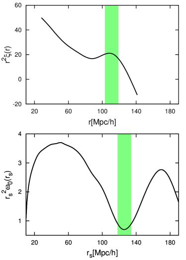
Figure 1: The standard two-point correlation function of DM haloes, $\xi(r)$ (upper panel), compared to the band-filtered correlation, $\omega_{0}(r_{s})$ (lower panel). Both statistics are computed in the $\Lambda$CDM scenario, at $z=0$. The green shaded bands mark the regions where the BAO feature is localized: a peak at $\sim 110$$h^{-1}\,\mbox{Mpc}$ in the $\xi(s)$ correlation function, a dip at $\sim 130$$h^{-1}\,\mbox{Mpc}$ in $\omega_{0}(r_{s})$.

The time evolution of linear density perturbations in the coupled CDM fluid and in the uncoupled baryonic component ($\delta_{c,b}\equiv\delta\rho_{c,b}/\rho_{c,b}$) is described at sub-horizon scales and in Fourier space by the following equations:

$$\ddot{\delta}_{c} = -2H\left[1-\eta_{c}\frac{\dot{\phi}}{H\sqrt{6}}\right]\dot{\delta}_{c}+4\pi G\left[\rho_{b}\delta_{b}+\rho_{c}\delta_{c}\Gamma_{c}\right]\,,$$ (10)

$$\ddot{\delta}_{b} = -2H\dot{\delta}_{b}+4\pi G\left[\rho_{b}\delta_{b}+\rho_{c}\delta_{c}\right]\,,$$ (11)

where, for simplicity, the dependence of the coupling function $\eta(\phi)$ has been omitted. The factor $\Gamma_{c}\equiv 1+4\eta_{c}^{2}(\phi)/3$ in Eq. (10) represents the fifth-force mediated by the DE scalar field, while the second term in the first square bracket at the right-hand-side of Eq. (10) is the extra-friction on CDM fluctuations arising as a consequence of momentum conservation (see e.g. Amendola, 2004; Pettorino & Baccigalupi, 2008; Baldi et al., 2010, 2011). A detailed description of the background and of the evolution of linear perturbations of all the cosmologies considered in this work can be found in Baldi (2012c) and Baldi (2012a).

3 The N-body simulations

Similarly to all the other DE models proposed in the last decades, the cDE scenarios investigated in this work are barely distinguishable from the $\Lambda$CDM model from their background expansion history. Furthermore, despite the fact that such cosmologies determine a different growth of linear density perturbations as compared to the concordance $\Lambda$CDM scenario, such effect is highly degenerate with standard cosmological parameters like $\Omega_{M}$ and, most importantly, $\sigma_{8}$. Hence, to discriminate between these cosmologies and the $\Lambda$CDM one, it is useful to exploit also the non-linear regime of structure formation, which requires to rely on large numerical simulations to accurately model all the non-linearities involved. The analysis described in the following sections is based on the public halo catalogues of the CoDECS simulations (Baldi, 2012c), the largest N-body runs for cDE cosmologies to date. The range of cosmological models considered in the CoDECS project, which includes the $\Lambda$CDM model as fiducial reference, and the constant, exponential and bouncing cDE cosmologies, are summarized in Table 1 along with their respective parameters. The viability of these models in terms of CMB observables has yet to be properly investigated, in particular for what concerns the impact of variable-coupling and bouncing cDE models on the large-scale power of CMB anisotropies. Although such analysis might possibly lead to tighter bounds on the coupling and on the potential functions than the ones allowed in the present work, here we are mainly interested in understanding the impact of cDE scenarios on the statistical properties of large-scale structures at late times, with a particular focus on the role played by non-linear effects, and we deliberately choose quite extreme values of the models parameters in order to maximize the effects under investigation.

The simulation suite considered in this work is the L-CoDECS series, a set of collisionless N-body runs in a cosmological box of 1 $h^{-1}\,\mbox{Gpc}$ on a side, with $1024^{3}$ CDM particles and $1024^{3}$ baryonic particles, a mass resolution of $m_{c}(z=0)=5.84\times 10^{10}$ M${}_{\odot}/h$ and $m_{b}=1.17\times 10^{10}$ M${}_{\odot}/h$ for CDM and baryons, respectively, and a force resolution of $\epsilon_{g}=20$ kpc$/h$. The simulations have been carried out with a modified version of the widely used parallel Tree-PM N-body code GADGET (Springel, 2005; Baldi et al., 2010).

The set of cosmological parameters at $z=0$ assumed in the CoDECS project are: $H_{0}=70.3\rm\,km\,s^{-1}\,Mpc^{-1}$, $\Omega_{\rm CDM}=0.226$, $\Omega_{\rm DE}=0.729$, $\sigma_{8}=0.809$, $\Omega_{b}=0.0451$ and $n_{s}=0.966$, consistent with the “CMB-only Maximum Likelihood” results of WMAP7 (Komatsu et al., 2011). All the L-CoDECS simulations are normalized at $z=z_{\rm CMB}$, using the same initial linear power spectrum, and then rescaling the resulting displacements to the starting redshift of the simulations, $z_{i}=99$, with the specific growth factor $D_{+}(z)$ obtained for each cosmological model by numerically solving Eqs. (10, 11).

The CDM haloes have been identified with a standard Friends-of-Friends (FoF) algorithm (Davis et al., 1985), using a linking length $\lambda=0.2\times\bar{d}$, where $\bar{d}$ is the mean interparticle separation. The results presented in this paper have been obtained using mass-selected sub-halo catalogues, composed by the gravitationally bound substructures that the algorithm SUBFIND (Springel et al., 2001) identifies in each FoF halo. For all the simulations, we adopted the following mass range: $M_{\rm min}<M<M_{\rm max}$, where $M_{\rm min}=2.5\cdot 10^{12}M_{\odot}/h$ and $M_{\rm max}=3.6\cdot 10^{15},1.1\cdot 10^{15},4.9\cdot 10^{14},2.6\cdot 10^{14},1.8\cdot 10^{14}M_{\odot}/h$ at $z=0,0.55,1,1.6,2$, respectively. In this paper, we only use mock subhalo catalogues and do not investigate which type of galaxies or clusters are more suited to achieve the highest accuracy and optimize our results. We defer a detailed discussion on this topic to a future paper.

Figure 2: The survey geometry function $\Phi(r)$ computed with Eq. (17). The bin used for its computation is d$r=0.5$ $h^{-1}\,\mbox{Mpc}$ and $N_{R}=5N_{D}$, where $N_{D}$ and $N_{R}$ are the number of haloes and random points, respectively. As can be seen, $0\leq\Phi(r)\leq 1$ and $\Phi(r)\rightarrow 1$ when $r\rightarrow 0$.

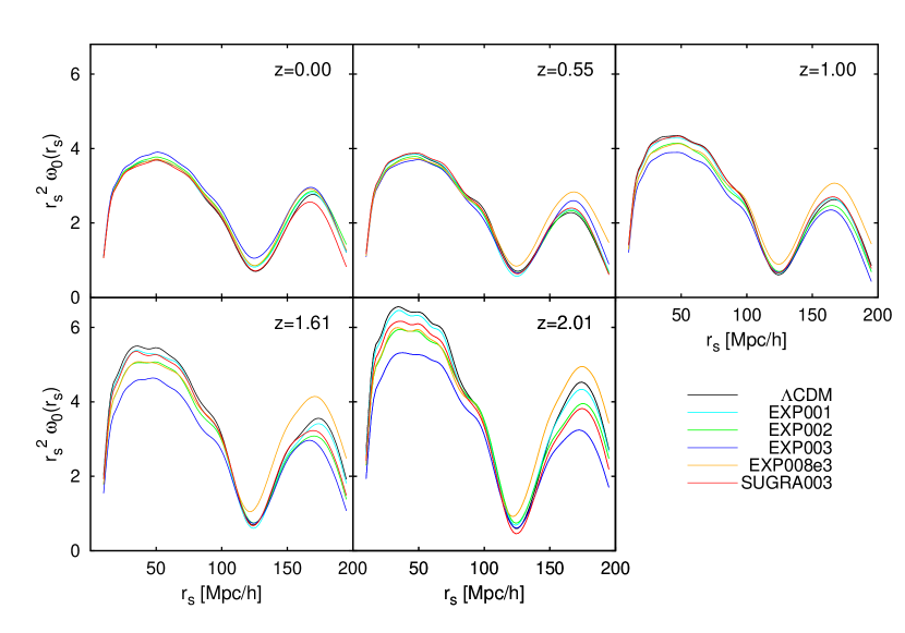
Figure 3: The band-filtered correlation function $\omega_{0}(r_{s})$ for the different cosmological models considered in the CoDECS simulations, measured in real-space. The BAO signal is clearly seen as a single dip. Different panels refer to different redshifts, as labelled.

4 The band-filtered correlation function

The simplest way to analyze the spatial properties of the LSS of the Universe is to use two-points statistics. The probability, $dP$, of finding a pair with one object in the volume $dV_{1}$ and the other in the volume $dV_{2}$, separated by a co-moving distance $r$, is given by:

$$dP=n^{2}[1+\xi(r)]dV_{1}dV_{2}\,,$$ (12)

where $\xi(r)$ is the two-point correlation function and $n$ is the number density of the objects. Xu et al. (2010) introduced a new statistic, $\omega_{l}(r_{s})$, to analyze the LSS and, in particular, the BAO, that presents some good advantages with respect to the traditional estimators, $\xi(r)$, and its Fourier transform, $P(k)$. In this paper, we will focus on the monopole $\omega_{l=0}(r_{s})$, that is directly linked to the traditional $\xi(r)$ and dominates the signal with respect to all higher-order terms (see Xu et al., 2010, for more details). The basic idea of this new statistic is to band-filter the acoustic information in the correlation function as follows:

$$\omega_{0}(r_{s})=4\pi\int_{0}^{r_{s}}\frac{dr}{r_{s}}\left(\frac{r}{r_{s}}\right)^{2}\xi(r)W(r,r_{s})\,.$$ (13)

The two-parameter filter function, $W(r,r_{s})$, must be compact and compensated ($\int r^{2}W(r,r_{s})dr=0$) with a characteristic scale $r_{s}$ (Padmanabhan et al., 2007). A convenient choice is to use the following analytical expression:

$$\left\{\begin{array}[]{ll}W(x)=4x^{2}(1-x)\left(\frac{1}{2}-x\right)&0<x<1\,,\\ W(x)=0&\textrm{otherwise}.\end{array}\right.$$ (14)

where $x=(r/r_{s})^{3}$. Figure 1 compares the standard two-point correlation function of DM haloes (upper panel) with the band-filtered correlation (lower panel). Both statistics are computed in the $\Lambda$CDM model, at $z=0$. While the BAO appears as a single peak, at $\sim 110$$h^{-1}\,\mbox{Mpc}$ , in the traditional $\xi(r)$, it is instead a single dip, at $\sim 130$$h^{-1}\,\mbox{Mpc}$ , in the new statistic $\omega_{0}(r_{s})$. It has been shown that $\omega_{0}(r_{s})$ combines the advantages of both the correlation function and the power spectrum approaches, at the same time (Xu et al., 2010; Blake et al., 2011). Indeed, $\omega_{0}(r_{s})$ is insensitive to small-scale power, which is difficult to model due to non-linear effects, and it is also insensitive to large-scale power, where it is slightly affected by the integral constraint. It is also easy to measure, as it only requires to weight the pair counts, without having to bin the data. If we adopt the natural estimator for the two-point correlation function:

$$\hat{\xi}(r,\mu)=\frac{DD(r,\mu)}{RR(r,\mu)}-1\,,$$ (15)

where $DD(r,\mu)$ and $RR(r,\mu)$ are the number of galaxy-galaxy and random-random pairs with separation $r$, and line-of-sight angle $\arccos(\mu)$, then from Eqs. (14) and (15) we can convert the integral given by Eq. (13) into the following expression:

$$\omega_{0}(r_{s})=\frac{2}{n_{D}N_{D}}\sum_{i=1}^{N}\frac{W(r_{i}/r_{s})}{\Phi(r_{i},\mu_{i})}\,,$$ (16)

where $N_{D}$ and $n_{D}$ are the number and number density of objects, respectively, and $\Phi(r,\mu)$ is a normalization function that encodes the geometry of the survey and depends on the number of data points. In general, $0\leq\Phi(r,\mu)\leq 1$ and when $r,\mu\rightarrow 0$, $\Phi(r,\mu)\rightarrow 1$. For simulations with periodic boundary conditions, $\Phi(r,\mu)=1$, as the volume is effectively infinite. The factor 2 appears because every pair is counted twice. The survey geometry function, $\Phi(r,\mu)$, can be estimated by filling the survey volume with randomly distributed points, taking into account that their number has to be much larger than the number of data points, in order to keep the shot noise in the random pairs smaller than in the object pairs. Hence, the function $\Phi(r,\mu)$ can be derived counting the random pairs, $RR$, and using the following equation:

$$RR(r,\mu)=2\pi n_{D}N_{D}r^{2}\Phi(r,\mu)\textrm{d}r\textrm{d}\mu\,,$$ (17)

where d$r$ and d$\mu$ are the bins used to count the $RR$ pairs in the survey. Notice that only the RR pairs, used to estimate the function $\Phi(r,\mu)$, are measured in finite bins, while the data are not binned, unlike the traditional correlation function measurements.

5 Results

5.1 Measuring the BAO scale in $\omega_{0}(r_{s})$

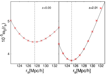
Figure 4: The band-filtered correlation function, $\omega_{0}(r_{s})$, in the $\Lambda$CDM cosmology, at $z=0$ and $z\sim 2$. Red stars show the measured $\omega_{0}(r_{s})$, while the black lines are the best-fit polynomial model. The vertical dotted lines mark the position of the BAO scale.

To construct mock halo catalogues from the snapshots of the CoDECS simulations, we locate virtual observers at $z=0$ and put each simulation box at a comoving distance corresponding to its output redshifts (see Marulli et al., 2012b; Bianchi et al., 2012, for a detailed discussion). With the above method, each snapshot box represents a finite volume of the Universe, and the survey geometry function, $\Phi(r,\mu)$, is not constant, as it would be if we measured the distances relying on the periodic boundary conditions. However, our simple mock geometry guarantees that $\Phi(r,\mu)$ is almost independent of $\mu$, as we have explicilty verified. We use Eq. (17) to estimate this survey geometry function, generating random catalogues five times larger than the halo ones and counting the number of random pairs in bins of d$r=0.5$ $h^{-1}\,\mbox{Mpc}$ . The result is shown in Fig. 2. We measure the band-filtered correlation function, $\omega_{0}(r_{s})$, using Eqs. (16) and (17), and linearly interpolating the function $\Phi(r)$ that we computed as just discussed. Fig. 3 shows the real-space $\omega_{0}(r_{s})$ of DM haloes, as a function of redshift ($z=\{0.00,\,0.55,\,1.00,\,1.61,\,2.01$}), measured in the range $10\leq r_{s}[$$h^{-1}\,\mbox{Mpc}$ $]\leq 190$. The black solid lines show the $\Lambda$CDM predictions, while the other curves refer to the cDE models of the CoDECS simulations, as reported by the labels. At small scales, $r_{s}\lesssim 50$ $h^{-1}\,\mbox{Mpc}$ , we confirm the results found by Marulli et al. (2012a) using the standard two-point correlation function. More specifically, we find that, at $z=0$, the small-scale halo spatial properties predicted by the cDE models are very similar to the $\Lambda$CDM ones. Going to higher redshifts, it is easier to discriminate between our DE models that predict different shapes of $\omega_{0}(r_{s})$. Future experiments, such as Euclid, will be able to accurately constrain the spatial properties of high redshift objects, thus helping in discriminating between alternative cosmological scenarios.

However, in this paper we are more interested in the horizontal shift of the BAO peak due to cDE non-linear dynamics, as this is not degenerate with $\sigma_{8}$, nor with the linear galaxy bias. So we will focus on low redshifts, where this effect is larger. To accurately localize the sound horizon scale in $r_{s}$-space, with the band-filtered correlation function (i.e the scale $r_{s}$ corresponding to the minimum value of $\omega_{0}(r_{s})$), we fitted the function $\omega_{0}(r_{s})$ around the dip using a polynomial function. As we are only interested in the position of the BAO feature, it is not necessary to model the shape of $\omega_{0}(r_{s})$ at all scales. Instead, we restrict our analyisis around the BAO dip: $|r_{s0}-r|\lesssim 5$$h^{-1}\,\mbox{Mpc}$ where $r_{s0}$ is the scale corresponding to the minimum value of $\omega_{0}(r_{s0})$. In the above range, the shape of band-filtered correlation function can be accurately modeled with a polynomial function of third order:

$$P_{3}(r_{s})=\sum_{i=0}^{4}a_{i}.r_{s}^{i}\,,$$ (18)

where $a_{i}$ are the coefficients of the polynomial. We estimate the $r_{s0}$ values for all the cosmological models considered in the CoDECS simulations and at different redshifts, fitting $\omega_{0}(r_{s})$ with the model given by Eq. (18) and finding the local minimum of the best-fit polynomials. As a case study, Fig. 4 shows the band-filtered correlation function around the dip, measured in the $\Lambda$CDM halo mock catalogues at $z=0$ and $z\sim 2$: red stars are the computed $\omega_{0}(r_{s})$, while the black lines show the best-fit polynomials. The vertical dotted lines mark the position of the BAO scale. As clearly shown in Fig. 4, the polynomial function is an excellent model for $\omega_{0}(r_{s})$ around the minimum.

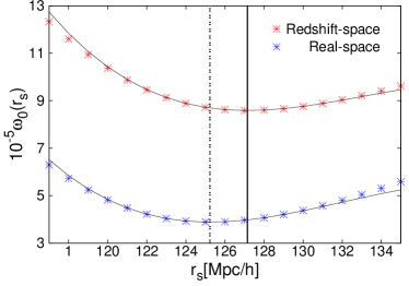
Figure 5: The band-filtered correlation functions in real- (blue stars) and redshift-space (red stars), for the $\Lambda$CDM cosmological model at $z=1$. Black lines are their fitting polynomials. The dotted (solid) vertical black line indicates the position of the BAO scale in real-space (redshift-space).

5.2 The shift of the BAO scale

5.2.1 The impact of non-linear dynamics

The BAO position changes slightly through cosmic time, as can be directly observed using numerical simulations. This shift is mainly driven by physical effects, as non-linear structure formation at large scales, that moves the position of the BAO signal to smaller scales relative to CMB-calibrated predictions. This occurs as a consequence of gravitational instability being non local (see e.g. Crocce & Scoccimarro, 2008). Therefore, at higher redshifts, where non-linearities have a small influence, the BAO peak in the two-point correlation function is located at larger scales than at lower redshifts. This effect can also be noticed in the band-filtered correlation function, with the difference that the BAO feature in $r_{s}$-space, i.e $r_{s0}$, is now located at smaller scales for higher redshifts, due to the effect of the filter, given by Eq.(14). This can be clearly seen in Fig. 4: the position of the BAO scale changes in time, from $r_{s0}\simeq 127.5$ at $z=0$ to $r_{s0}\simeq 125$ at $z=2$. In $r_{s}$-space, both the scale and the amplitude of the BAO feature increase as redshifts decrease.

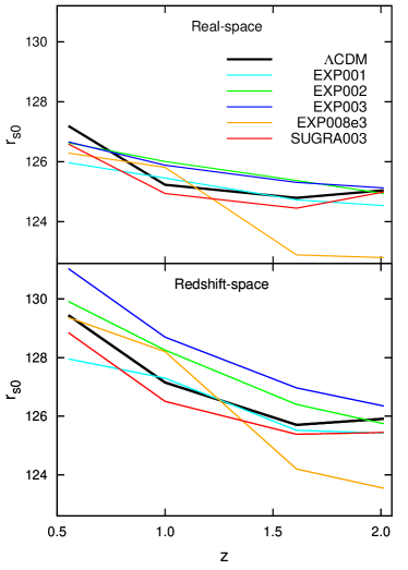
Figure 6: Evolution of the BAO scale in the band-filtered correlation function, due to non-linearities for real- (upper panel) and redshift-space (lower panel) from $z\sim 0.5$ to $z=2$.

5.2.2 The impact of redshift-space distortions

RSD induced by galaxy peculiar motions further shift the position of the BAO scale (Smith et al., 2008). To construct redshift-space halo mock catalogues, we estimate the observed redshift of each object via the following equation:

$$z_{obs}=z_{c}+\frac{\nu_{\|}}{c}(1+z_{c})\,,$$ (19)

where $z_{c}$ is the cosmological redshift due to the Hubble recession velocity at the comoving distance of the halo, $\nu_{\|}$ is the line-of-sight component of its centre of mass velocity and $c$ is the speed of light. Fig. 5 shows the effect of RSD on the BAO feature, for the $\Lambda$CDM model at $z=1$. Blue and red stars show the real- and redshift-space band-filtered correlation functions, respectively. The vertical dotted and solid black lines indicate the position of the BAO scale in real- and redshift-space, respectively. The amplitude enhancement of $\omega_{0}(r_{s})$ in redshift-space is caused by the Kaiser effect and is directly proportional to the linear growth rate of cosmic structures (Marulli et al., 2012a). Here, we are more interested in the horizontal shift, as this is not degenerate with $\sigma_{8}$, allowing to break the degeneracy between the effects arising as a consequence of the DE-CDM interactions and standard cosmological parameters. As shown in Fig. 5, the BAO scale is shifted by $\sim 2$ $h^{-1}\,\mbox{Mpc}$ from real- to redshift-space.

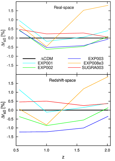
Figure 7: The percentage difference between cDE and $\Lambda$CDM model predictions of the evolution of the BAO scale in the band-filtered correlation function, due to non-linearities for real- and redshift-space from $z\sim 0.5$ to $z=2$.

5.3 The BAO scale as a dynamical probe

The shift of the BAO scale due to non-linearities and RSD depends directly on the underlying cosmology. When the BAO feature is used as a geometric standard ruler, it is necessary to accurately correct for the shift, to avoid systematics when constraining cosmological parameters. Most importantly, the correction should be different for each cosmological model to test. On the other hand, if the sound horizon scale is measured with sufficient accuracy, the BAO shift can provide a dynamical probe to discriminate between different cosmological models.

The interaction between DE and CDM shifts the matter-radiation equality to higher redshifts, as CDM dilutes faster relative to the $\Lambda$CDM case and there was more CDM in the past (see e.g. Amendola et al., 2012a). Moreover, in cDE models the evolution of linear and non-linear density perturbations is significantly altered, as compared to the standard $\Lambda$CDM scenario. Specifically, as discussed in §2, the DE coupling induces a time evolution of the mass of CDM particles as well as a modification of the growth of structures, determined by the combined effect of a long-range fifth-force, mediated by the DE scalar degree of freedom, and of an extra-friction, arising as a consequence of momentum conservation. At large scales, these effects change the location and the amplitude of the BAO scale. Therefore, the clustering properties of CDM haloes at the sound horizon scale, in particular the combination of the BAO shifts due to non-linearities and RSD, might show specific signatures, allowing to distinguish a cDE Universe from the $\Lambda$CDM scenario.

5.3.1 The cDE BAO in real- and redshift-space

Using our mock halo catalogues, we can quantify the effect of non-linear dynamics in the band-filtered correlation function, for the different cDE models of the CoDECS project. Fig. 6 shows the evolution of the position of the BAO scale, $\mathrm{r_{s0}}$, in real- (upper panel) and redshift-space (lower panel), as a function of redshift and cosmological model. In both panels we can see that $\mathrm{r_{s0}}$ increases, due to non-linearities, as redshift decreases. Comparing the upper and lower panel, we can see the impact of the RSD on the position of $\mathrm{r_{s0}}$ for every cosmological model from $z\sim 0$ to $z\sim 2$, i.e. the shifts of $\mathrm{r_{s0}}$ to higher scales from real- to redshift-space as described in §5.2.2.

In Fig. 7, we show the percentage difference between cDE and $\Lambda$CDM predictions, $\mathrm{\Delta r_{s0}=100\cdot(r_{s0,cDE}-r_{s0,\Lambda CDM})/r_{s0,\Lambda CDM}}$, where $\mathrm{r_{s0,\Lambda CDM}}$ is the $\Lambda$CDM BAO scale, and $\mathrm{r_{s0,cDE}}$ its counterpart for every cDE model. The percentage differences between the values of $\mathrm{r_{s0}}$ in $\Lambda$CDM and cDE models are quite small, $\lesssim 2\%$ in the whole redshift range. The EXP008e3 model predicts the largest difference, that rises from $\sim 1\%$ to $\sim 2\%$ at $z\sim 1.5$ and $z\sim 2$, respectively. The $\mathrm{r_{s0}}$ difference in the SUGRA003 scenario is always positive ($\lesssim 0.5\%$) and almost constant up to $z\sim 0.5$.

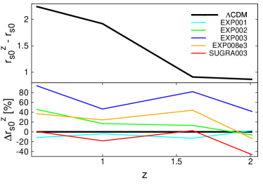
Figure 8: Upper panel: The evolution of the difference between the sound horizon scale in redshift- and real-space for the $\Lambda$CDM scenario. Bottom panel: Percentage difference between cDE models and $\Lambda$CDM model predictions obtained from the Eq. (20).

The most interesting result of Fig. 6 is the amplification effect of RSD. While, in real-space, $\mathrm{\Delta r_{s0}}$ is small for all the cDE models considered (except for EXP008e3, at high redshifts), the predictions of the different cDE models are much more clearly distinguishable in redshift-space. To better quantify this effect, in Fig. 8 we show the difference between the sound horizon scale in redshift- and real-space. RSD move the sound horizon at larger scales (as highlighted by the black line in the upper panel, that shows the $\Lambda$CDM prediction), an effect that monotonically increases at low redshifts. More interestingly, the effect of RSD is strongly model-dependent, as can be clearly seen in the lower panel of Fig. 8, that shows the percentage difference between $\mathrm{\Delta r_{s0}}$ in $\Lambda$CDM and cDE models:

$$\mathrm{\Delta r^{z}_{s0}=100\cdot\frac{(r^{z}_{s0,cDE}-r_{s0,cDE})-(r^{z}_{s0,\Lambda CDM}-r_{s0,\Lambda CDM})}{{(r^{z}_{s0,\Lambda CDM}-r_{s0,\Lambda CDM})}}}\,,$$ (20)

where $\mathrm{r^{z}_{s0,\Lambda CDM}}$ and $\mathrm{r_{s0,\Lambda CDM}}$ are the positions of the BAO feature in redshift- and real-space respectively, in the $\Lambda$CDM scenario, while $\mathrm{r^{z}_{s0,cDE}}$ and $\mathrm{r_{s0,cDE}}$ are their respective counterparts for every cDE scenario.

For constant coupling models, the RSD effect is directly proportional to the coupling strength, $\beta$: the larger is $\beta$, the most the BAO scale is shifted to large scales. Indeed, the strongest effect is found for the EXP003 model, over the whole redshift range, for which the BAO shift due to RSD is up to $\sim 90\%$. On the other hand, the impact of RSD is almost negligible for the EXP001 and SUGRA003 models. We note that $\mathrm{\Delta r_{s0}}$ can be negative for these models, but the effect is small considering the statistical uncertainties.

5.3.2 The impact of redshift errors

As we have seen in the previous sections, non-linear small-scale effects can “propagate” to larger scales, significantly shifting the sound horizon in a cosmology-dependent way. Hence, it is mandatory to investigate how redshift errors can impact the BAO feature. Here we consider only Gaussian redshift errors, typical of both spectroscopic and photometric galaxy surveys, and do not investigate the impact of the so-called catastrophic errors (the ones caused by the misidentification of one or more spectral features). Indeed, pure catastrophic outliers with a flat distribution simply reduce the amplitude of $\omega_{0}(r_{s})$ at all scales, not affecting the position of $r_{s0}$. On the other hand, BAO shifts possibly induced by systematic misidentifications of spectral features need to be estimated with mock galaxy catalogues, taking into account the specific observational effects of the survey under investigation.

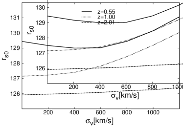
Figure 9: The impact of redshift errors on the position of the BAO scale, for the $\Lambda$CDM model at different reshifts ($z=0.55$ - solid line, $z=1$ - dotted line, $z=2$ - dot-dashed line).

We estimate the redshift of each mock halo with a modified version of Eq. 19:

$$z_{obs}=z_{c}+\frac{\nu_{\|}}{c}(1+z_{c})+\frac{\sigma_{v}}{c}\,,$$ (21)

where the new term $\sigma_{v}$ is the random error in the measured redshift (expressed in km/s). To assess the impact of redshift errors on the position of $\mathrm{r_{s0}}$, we measure the band-filtered correlation in halo mock catalogues with the following Gaussian redshift errors: $\sigma_{v}=\{0,200,400,600,800,1200\}$ km/s. In Fig 9, we show our results only for the $\Lambda$CDM scenario, as the effect of redshift errors does not depend on the cosmological model. The impact of Gaussian errors results to be negligible for $\sigma_{v}\lesssim 600$ km/s and, at high redshifts ($z\gtrsim 1.5$), even for larger values of $\sigma_{v}$. On the other hand, for $z\lesssim 1$ and $\sigma_{v}\gtrsim 600$ km/s, the sound horizon systematically shifts to larger scales as redshift errors increase. Typical spectroscopic galaxy surveys have quite accurate redshift measurements ($\sigma_{v}<100$ km/s), hence the systematic effect of redshift errors at the BAO scale is tiny in these cases. However, larger redshift errors, typical of photometric surveys, could introduce a non-negligible shift in the sound horizon scale, that should be accurately corrected when extracting cosmological constraints from the BAO feature. Interestingly, if we consider the required redshift error limits of the Euclid surveys, i.e. $\sigma_{z}\leq 0.001(1+z)$, which corresponds to 600 km/s at $z=1$ (Laureijs et al., 2011), the error on the location of $\mathrm{r_{s0}}$ is $\sim 0.5$%, i.e. small enough to distinguish cDE models from the $\Lambda$CDM scenario.

6 Conclusions

In this paper, we quantified the impact of DE interactions on the clustering of CDM haloes at large scales, using the band-filtered correlation function $\omega_{0}(r_{s})$. We used the public halo catalogues from the CoDECS simulations, a suite of large N-body runs for cDE models. We accurately estimated the sound horizon scale in our mock halo catalogues, fitting the function $\omega_{0}(r_{s})$ with third order polynomials around the BAO scale. We investigated the effects of non-linear dynamics both in real- and redshift-space, in the ranges $10\lesssim r_{s}\lesssim 190$ and $0\leq z\leq 2$. The main results of our analysis are the following.

• We detected BAO shifts in $\omega_{0}(r_{s})$, relative to the linear predictions, for $\Lambda$CDM and cDE cosmologies: non-linear effects shift the sound horizon to larger scales, an effect that monotonically increases moving to lower redshifts.

• RSD significantly amplify the non-linear BAO shift, at all redshifts. On the other hand, Gaussian redshift errors $\lesssim 600$ km/s have a negligible impact at the BAO scale.

• The combined BAO shift due to non-linearities and RSD is strongly model dependent. Thus, if the BAO scale is accurately measured, it can provide a tool to distinguish between $\Lambda$CDM and cDE models.

To conclude, besides the common use as a standard ruler, the BAO feature can be exploited also as a dynamical probe to disentangle between cosmological scenarios characterized by different non-linear dynamics. The BAO shift due to cDE dynamics is generally small, but RSD significantly amplify the effect, expecially at low redshifts. Moreover, the shift of the BAO scale is not degenerate with $\sigma_{8}$ and, consequently, with the other paratemeters degenerate in turn with $\sigma_{8}$, like the linear galaxy bias and the total mass of neutrinos (La Vacca et al., 2009; Kristiansen et al., 2010; Marulli et al., 2011). Thus, the BAO feature provides a strong and unbiased probe for detecting new dark interactions, and can be of great help in removing the $\sigma_{8}$-degeneracy of other intependent observables, like the halo mass function (Cui et al., 2012) and the clustering anisotropies (Marulli et al., 2012a).

References

- Albrecht et al. (2006) Albrecht A., et al., 2006
- Amendola (2000) Amendola L., 2000, Phys. Rev. D, 62, 043511
- Amendola (2004) Amendola L., 2004, Phys. Rev., D69, 103524
- Amendola et al. (2008) Amendola L., Baldi M., Wetterich C., 2008, Phys. Rev. D, 78, 023015
- Amendola et al. (2012a) Amendola L., Pettorino V., Quercellini C., Vollmer A., 2012a, Phys. Rev. D, 85, 103008
- Amendola et al. (2012b) Amendola L., et al., 2012b, ArXiv e-prints
- Angulo et al. (2008) Angulo R. E., Baugh C. M., Frenk C. S., Lacey C. G., 2008, Mon. Not. R. Astron. Soc., 383, 755
- Baldi (2011) Baldi M., 2011, Mon. Not. R. Astron. Soc., 411, 1077
- Baldi (2012a) Baldi M., 2012a, Mon. Not. R. Astron. Soc., 420, 430
- Baldi (2012b) Baldi M., 2012b, Annalen der Physik, 524, 602
- Baldi (2012c) Baldi M., 2012c, Mon. Not. R. Astron. Soc., 422, 1028
- Baldi & Pettorino (2011) Baldi M., Pettorino V., 2011, Mon. Not. R. Astron. Soc., 412, L1
- Baldi et al. (2011) Baldi M., Pettorino V., Amendola L., Wetterich C., 2011, Mon. Not. R. Astron. Soc., 1444
- Baldi et al. (2010) Baldi M., Pettorino V., Robbers G., Springel V., 2010, Mon. Not. R. Astron. Soc., 403, 1684
- Beutler et al. (2011) Beutler F., et al., 2011, Mon. Not. R. Astron. Soc., 416, 3017
- Bianchi et al. (2012) Bianchi D., Guzzo L., Branchini E., Majerotto E., de la Torre S., Marulli F., Moscardini L., Angulo R. E., 2012, ArXiv e-prints
- Blake et al. (2011) Blake C., et al., 2011, Mon. Not. R. Astron. Soc., 415, 2892
- Boylan-Kolchin et al. (2011) Boylan-Kolchin M., Bullock J. S., Kaplinghat M., 2011, arXiv:1111.2048
- Brax & Martin (1999) Brax P. H., Martin J., 1999, Physics Letters B, 468, 40
- Brookfield et al. (2008) Brookfield A. W., van de Bruck C., Hall L. M. H., 2008, Phys. Rev., D77, 043006
- Caldera-Cabral et al. (2009) Caldera-Cabral G., Maartens R., Urena-Lopez L. A., 2009, Phys. Rev., D79, 063518
- Cole et al. (2005) Cole S., et al., 2005, Mon. Not. R. Astron. Soc., 362, 505
- Crocce & Scoccimarro (2008) Crocce M., Scoccimarro R., 2008, Phys. Rev. D, 292, 023533
- Cui et al. (2012) Cui W., Baldi M., Borgani S., 2012, Mon. Not. R. Astron. Soc., 424, 993
- Damour et al. (1990) Damour T., Gibbons G. W., Gundlach C., 1990, Phys. Rev. Lett., 64, 123
- Davis et al. (1985) Davis M., Efstathiou G., Frenk C. S., White S. D. M., 1985, Astrophys. J., 292, 371
- Eisenstein et al. (2005) Eisenstein D. J., et al., 2005, Astrophys. J., 633, 560
- Ettori (2003) Ettori S., 2003, Mon. Not. R. Astron. Soc., 344, L13
- Farrar & Peebles (2004) Farrar G. R., Peebles P. J. E., 2004, Astrophys. J., 604, 1
- Farrar & Rosen (2007) Farrar G. R., Rosen R. A., 2007, Physical Review Letters, 98, 171302
- Gaztañaga et al. (2009) Gaztañaga E., Cabré A., Hui L., 2009, Mon. Not. R. Astron. Soc., 399, 1663
- Hütsi (2006) Hütsi G., 2006, Astron. Astrophys., 449, 891
- Kazin et al. (2010) Kazin E. A., et al., 2010, Astrophys. J., 710, 1444
- Komatsu et al. (2011) Komatsu E., et al., 2011, Astrophys. J. Suppl., 192, 18
- Koyama et al. (2009) Koyama K., Maartens R., Song Y.-S., 2009, JCAP, 0910, 017
- Kristiansen et al. (2010) Kristiansen J. R., La Vacca G., Colombo L. P. L., Mainini R., Bonometto S. A., 2010, New Astron., 15, 609
- La Vacca et al. (2009) La Vacca G., Kristiansen J. R., Colombo L. P. L., Mainini R., Bonometto S. A., 2009, J. Cosm. Astro-Particle Phys., 4, 7
- Laureijs et al. (2011) Laureijs R., et al., 2011, ArXiv e-prints
- Lee & Baldi (2011) Lee J., Baldi M., 2011, ArXiv e-prints
- Lee & Komatsu (2010) Lee J., Komatsu E., 2010, Astrophys. J., 718, 60
- Lucchin & Matarrese (1985) Lucchin F., Matarrese S., 1985, Phys. Rev. D, 32, 1316
- Macciò et al. (2004) Macciò A. V., Quercellini C., Mainini R., Amendola L., Bonometto S. A., 2004, Phys. Rev., D69, 123516
- Marulli et al. (2012a) Marulli F., Baldi M., Moscardini L., 2012a, Mon. Not. R. Astron. Soc., 420, 2377
- Marulli et al. (2012b) Marulli F., Bianchi D., Branchini E., Guzzo L., Moscardini L., Angulo R. E., 2012b, Mon. Not. R. Astron. Soc., 426, 2566
- Marulli et al. (2011) Marulli F., Carbone C., Viel M., Moscardini L., Cimatti A., 2011, Mon. Not. R. Astron. Soc., 418, 346
- McCarthy et al. (2007) McCarthy I. G., Bower R. G., Balogh M. L., 2007, Mon. Not. R. Astron. Soc., 377, 1457
- Navarro et al. (1996) Navarro J. F., Frenk C. S., White S. D. M., 1996, Astrophys. J., 462, 563
- Okumura et al. (2008) Okumura T., Matsubara T., Eisenstein D. J., Kayo I., Hikage C., Szalay A. S., Schneider D. P., 2008, Astrophys. J., 676, 889
- Padmanabhan & White (2009) Padmanabhan N., White M., 2009, Phys. Rev. D, 80, 063508
- Padmanabhan et al. (2007) Padmanabhan N., et al., 2007, Mon. Not. R. Astron. Soc., 378, 852
- Peebles & Yu (1970) Peebles P., Yu J. T., 1970, Astrophys. J., 162, 815
- Percival et al. (2007) Percival W. J., Cole S., Eisenstein D. J., Nichol R. C., Peacock J. A., Pope A. C., Szalay A. S., 2007, Mon. Not. R. Astron. Soc., 381, 1053
- Percival et al. (2010) Percival W. J., et al., 2010, Mon. Not. R. Astron. Soc., 401, 2148
- Perlmutter et al. (1999) Perlmutter S., et al., 1999, Astrophys. J., 517, 565
- Pettorino & Baccigalupi (2008) Pettorino V., Baccigalupi C., 2008, Phys. Rev. D, 77, 103003
- Riess et al. (1998) Riess A. G., et al., 1998, Astron. J., 116, 1009
- Sánchez et al. (2009) Sánchez A. G., Crocce M., Cabré A., Baugh C. M., Gaztañaga E., 2009, Mon. Not. R. Astron. Soc., 400, 1643
- Schlegel et al. (2011) Schlegel D., et al., 2011, ArXiv e-prints
- Schmidt et al. (1998) Schmidt B. P., et al., 1998, Astrophys.J., 507, 46
- Seo & Eisenstein (2003) Seo H.-J., Eisenstein D. J., 2003, Astrophys. J., 598, 720
- Seo & Eisenstein (2005) Seo H.-J., Eisenstein D. J., 2005, Astrophys. J., 633, 575
- Smith et al. (2008) Smith R., Scoccimarro R., Sheth R., 2008, Phys. Rev. D, 77, 043525
- Springel (2005) Springel V., 2005, Mon. Not. R. Astron. Soc., 364, 1105
- Springel et al. (2001) Springel V., Yoshida N., White S. D. M., 2001, New Astronomy, 6, 79
- Watkins et al. (2009) Watkins R., Feldman H. A., Hudson M. J., 2009, Mon. Not. R. Astron. Soc., 392, 743
- Wetterich (1988) Wetterich C., 1988, Nuclear Physics B, 302, 668
- Wetterich (1995) Wetterich C., 1995, Astron. Astrophys., 301, 321
- Xu et al. (2010) Xu X., et al., 2010, Astrophys. J., 718, 1224