Framed link presentations of 3-manifolds by an ${O}(n^{2})$ algorithm, III: geometric complex $\mathcal{H}_{n}^{\star}$ embedded into $\mathbb{R}^{3}$

Abstract

In this final part of a 3-part paper we introduce the pair of “wings” of the abstract PL-colored complexes $\mathcal{H}_{m}^{\star}$, described in the second paper. The wings, via a weight enhanced Tutte’s barycentric embedding of a planar map, produce the unexpected reformutation of a 3-dimensionl problem into a 2-dimensional one. The total number of edges in each one of the pair of final wings is less than $8n-5$. Tutte’s method is applied $O(n)$ times to each one of the 2 wings in the final pair to assure rectilinearity of the embeddings of the planar maps, which include the final wings. A cone construction over the final wings provides a PL-complex $\mathcal{H}_{1}^{\diamond}$, which contain the set of 0-simplices $\{a_{1},a_{2},\ldots,a_{f}\}\cup\{b_{1},b_{2},\ldots,b_{g}\}$ (as defined in the second part of the article) properly fixed in $\mathbb{R}^{3}$. The other 0-simplices are obtained by bisections of segments linking previously defined points. This implies that $\mathcal{H}_{n}$ is PL-embedded into $\mathbb{R}^{3}$. We then conclude the surgery description of the 3-manifold induced by the gem with its resolution by defining some disjoint cylinders contained in $\mathcal{H}_{n}^{\star}$, directly from the hinges (dual of the twistors of the resolution), in a 1-1 correspondence. The medial curves of the cylinders define the link we seek. The framing of a medial curve is the linking number of the boundary components of the corresponding cylinder. The analysis of the whole proccess shows that the memory and time requirement to complete the algorithm is $O(n^{2})$. Data for the Weber-Seifert 3-manifold, which answers Jeffrey Weeks’s question is given in the appendix. It consists of a link with 142 crossings but it admits simplifications.

1 Wings as seeds for obtaining the dual PL-complex $\mathcal{H}_{n}^{\star}$

This is the third of 3 closely related articles. References for the companion papers are [6] and [7].

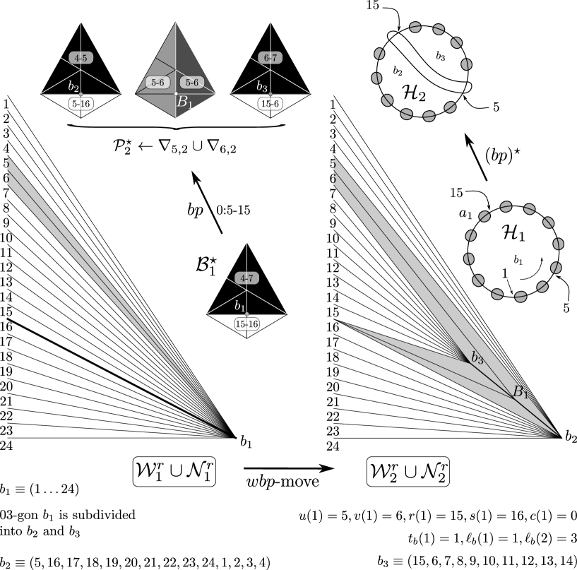
Figure 19: $\mathcal{H}^{\star}_{2}\leftarrow\mathcal{H}^{\star}_{1}\cup(\mathcal{P}_{2}^{\star}\backslash\mathcal{B}_{1}^{\star})$. Pillow $\mathcal{P}_{2}^{\star}\leftarrow\nabla_{5,12}\cup\nabla_{6,12}$ ($r^{24}_{5}$-example).

Let $\Pi_{\ell}$ ($\Pi_{r}$) be the half plane limited by the $z$-axis which contains $a_{1}=z_{0}z_{2}/2$ $(b_{1}=z_{1}z_{2}/2)$. The construction of the wings and nervures of the next section are exemplified in Figs. 19 to 29.

1.1 Wings: reformulating a difficult 3D-problem into an easy planar one

At some point in our research it became evident that what was needed to obtain the PL-complex $\mathcal{H}_{n}^{\star}$ was a proper embedding into $\mathbb{R}^{3}$ of the set of 0-simplices $\{a_{1},a_{2},\ldots,a_{f}\}\cup\{b_{1},b_{2},\ldots,b_{g}\}$. The other 0-simplices are obtained by bisections of segments linking previously defined points. It came as a surprise to discover that this apparently difficult 3D problem was reformulated as a plane problem for which we had at hand an easy solution, namely Tutte’s barycentric method.

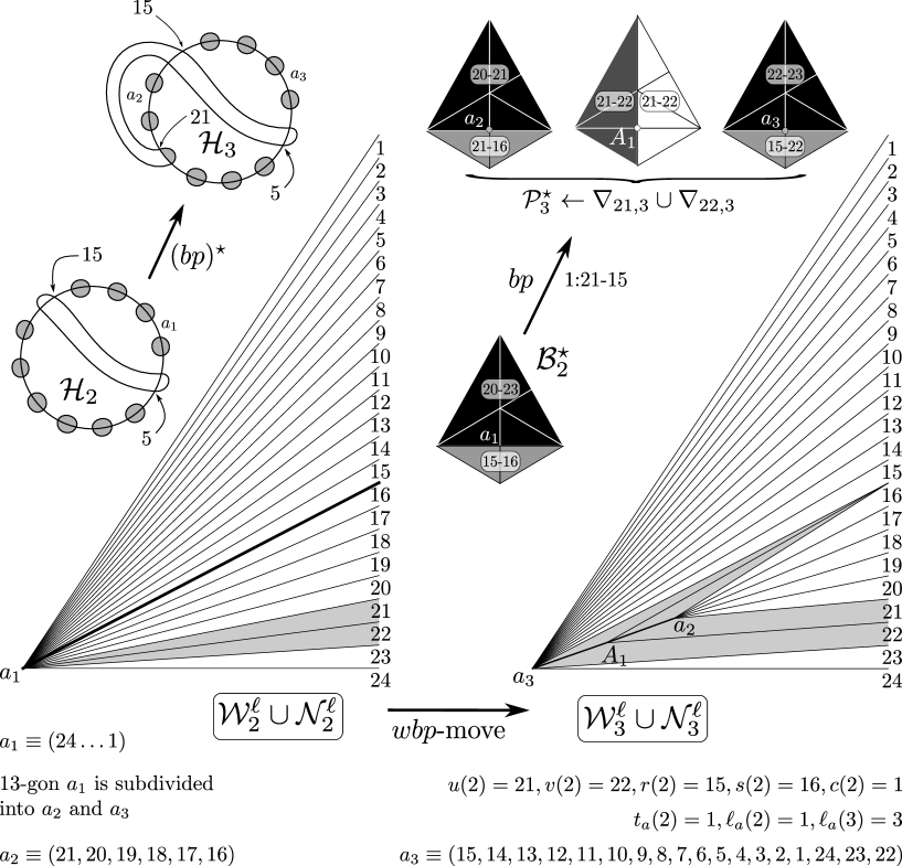
Figure 20: $\mathcal{H}^{\star}_{3}\leftarrow\mathcal{H}^{\star}_{2}\cup(\mathcal{P}_{3}^{\star}\backslash\mathcal{B}_{2}^{\star})$. Pillow $\mathcal{P}_{3}^{\star}\leftarrow\nabla_{21,12}\cup\nabla_{22,12}$ ($r^{24}_{5}$-example).

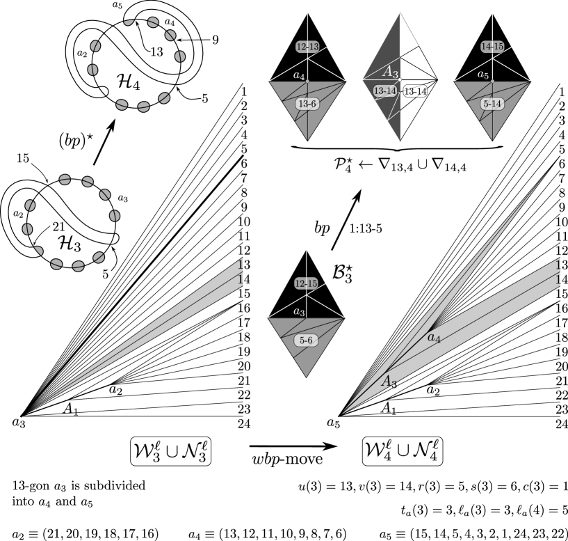
Figure 21: $\mathcal{H}^{\star}_{4}\leftarrow\mathcal{H}^{\star}_{3}\cup(\mathcal{P}_{4}^{\star}\backslash\mathcal{B}_{3}^{\star})$. Pillow $\mathcal{P}_{4}^{\star}\leftarrow\nabla_{13,12}\cup\nabla_{14,12}$ ($r^{24}_{5}$-example).

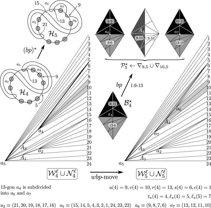
Figure 22: $\mathcal{H}^{\star}_{5}\leftarrow\mathcal{H}^{\star}_{4}\cup(\mathcal{P}_{5}^{\star}\backslash\mathcal{B}_{4}^{\star})$. Pillow $\mathcal{P}_{5}^{\star}\leftarrow\nabla_{9,12}\cup\nabla_{10,12}$ ($r^{24}_{5}$-example).

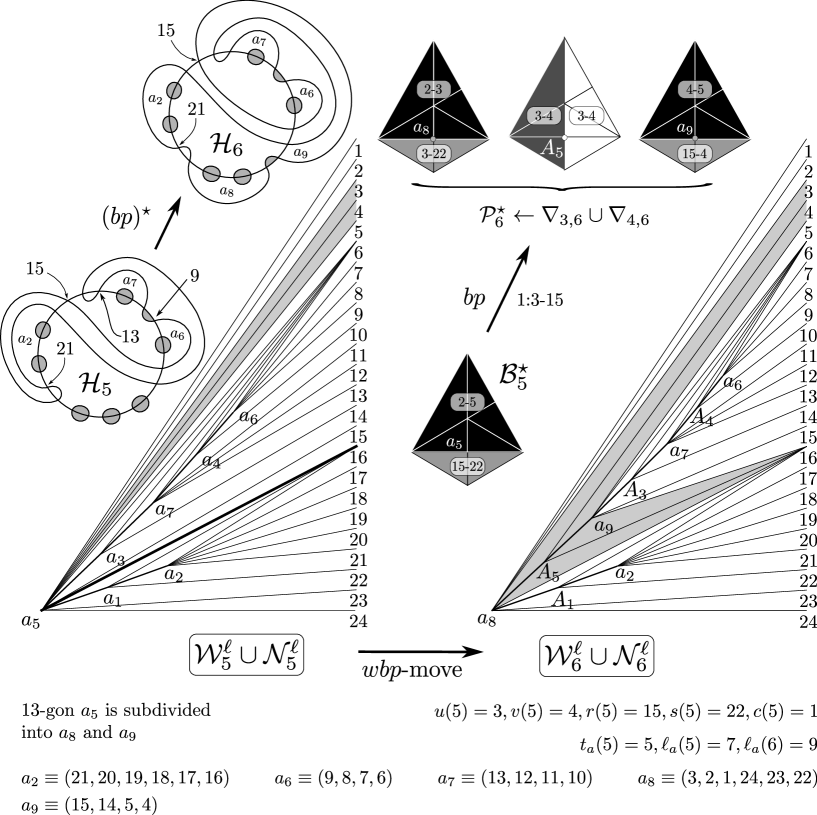
Figure 23: $\mathcal{H}^{\star}_{6}\leftarrow\mathcal{H}^{\star}_{5}\cup(\mathcal{P}_{6}^{\star}\backslash\mathcal{B}_{5}^{\star})$. Pillow $\mathcal{P}_{6}^{\star}\leftarrow\nabla_{3,12}\cup\nabla_{4,12}$ ($r^{24}_{5}$-example).

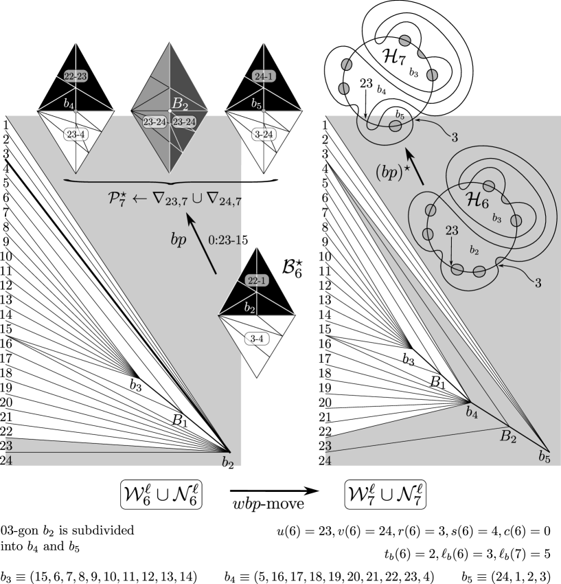
Figure 24: $\mathcal{H}^{\star}_{7}\leftarrow\mathcal{H}^{\star}_{6}\cup(\mathcal{P}_{7}^{\star}\backslash\mathcal{B}_{6}^{\star})$. Pillow $\mathcal{P}_{7}^{\star}\leftarrow\nabla_{23,12}\cup\nabla_{24,12}$ ($r^{24}_{5}$-example).

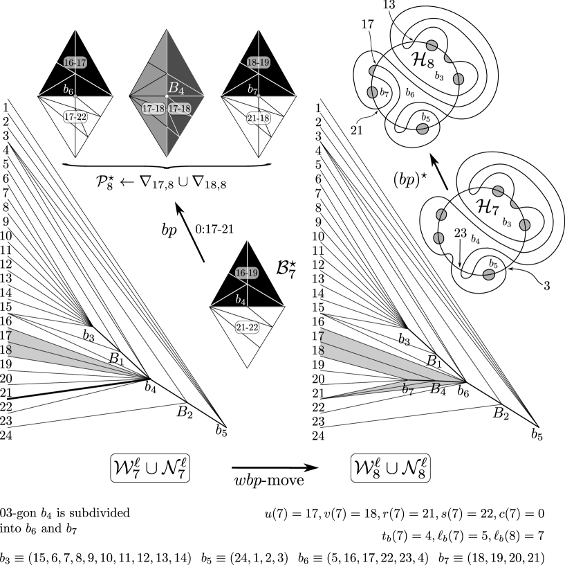
Figure 25: $\mathcal{H}^{\star}_{8}\leftarrow\mathcal{H}^{\star}_{7}\cup(\mathcal{P}_{8}^{\star}\backslash\mathcal{B}_{7}^{\star})$. Pillow $\mathcal{P}_{8}^{\star}\leftarrow\nabla_{17,12}\cup\nabla_{18,12}$ ($r^{24}_{5}$-example).

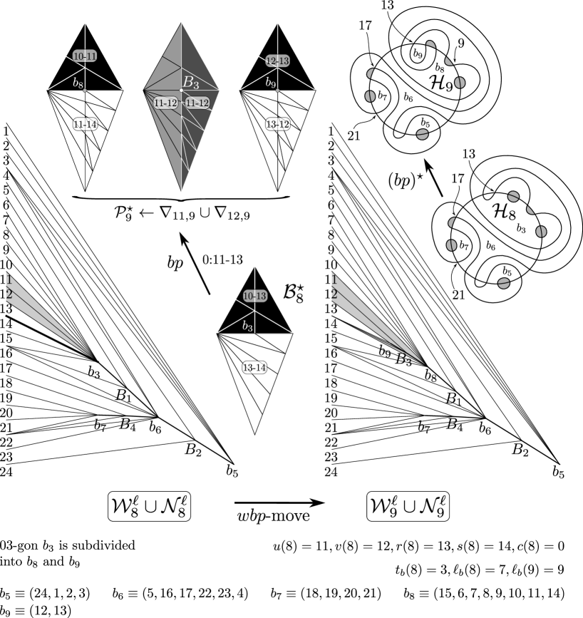
Figure 26: $\mathcal{H}^{\star}_{9}\leftarrow\mathcal{H}^{\star}_{8}\cup(\mathcal{P}_{9}^{\star}\backslash\mathcal{B}_{8}^{\star})$. Pillow $\mathcal{P}_{9}^{\star}\leftarrow\nabla_{11,12}\cup\nabla_{12,12}$ ($r^{24}_{5}$-example).

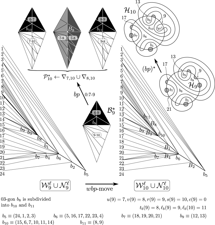
Figure 27: $\mathcal{H}^{\star}_{10}\leftarrow\mathcal{H}^{\star}_{9}\cup(\mathcal{P}_{10}^{\star}\backslash\mathcal{B}_{9}^{\star})$. Pillow $\mathcal{P}_{10}^{\star}\leftarrow\nabla_{7,12}\cup\nabla_{8,12}$ ($r^{24}_{5}$-example).

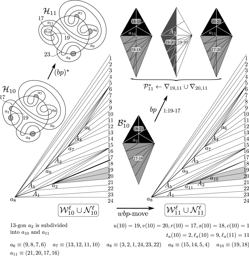
Figure 28: $\mathcal{H}^{\star}_{11}\leftarrow\mathcal{H}^{\star}_{10}\cup(\mathcal{P}_{11}^{\star}\backslash\mathcal{B}_{10}^{\star})$. Pillow $\mathcal{P}_{11}^{\star}\leftarrow\nabla_{19,12}\cup\nabla_{20,12}$ ($r^{24}_{5}$-example).

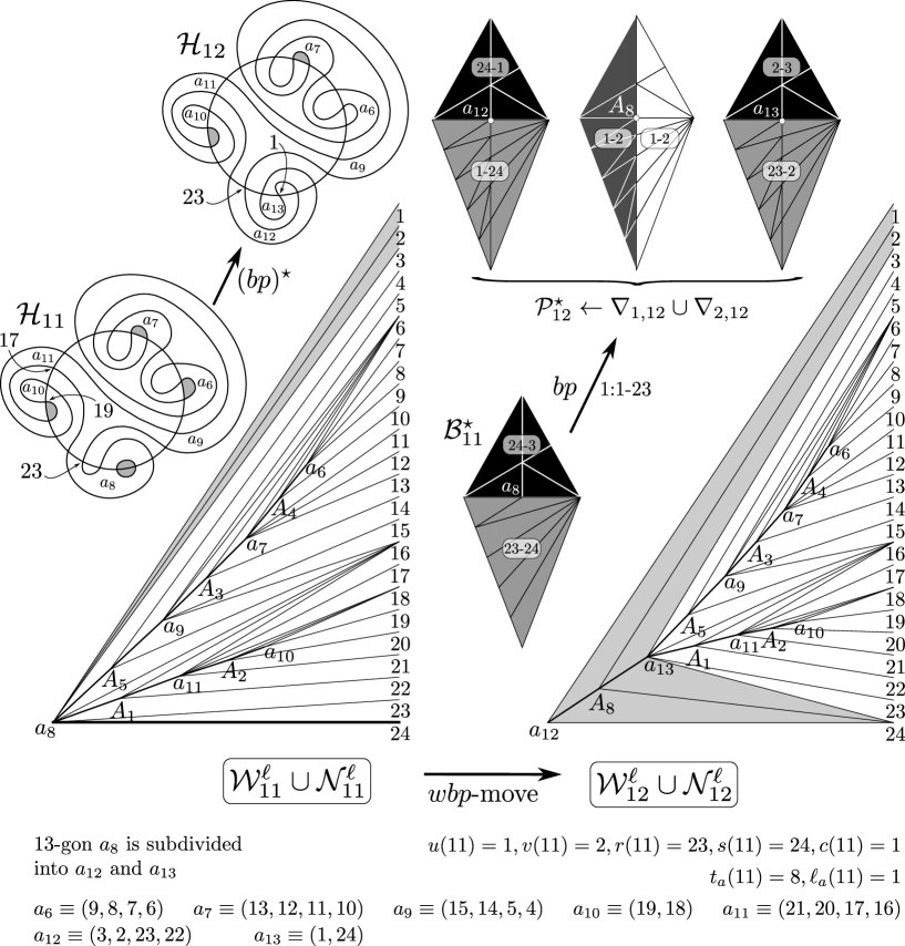
Figure 29: $\mathcal{H}^{\star}_{12}\leftarrow\mathcal{H}^{\star}_{11}\cup(\mathcal{P}_{12}^{\star}\backslash\mathcal{B}_{11}^{\star})$. Pillow $\mathcal{P}_{12}^{\star}\leftarrow\nabla_{1,12}\cup\nabla_{2,12}$ ($r^{24}_{5}$-example).

We construct a sequence pairs of plane graphs $\{\{\mathcal{W}^{\ell}_{1},\mathcal{W}^{r}_{1}\},\{\mathcal{W}^{\ell}_{2},\mathcal{W}^{r}_{2}\},\ldots,\{\mathcal{W}^{\ell}_{n},\mathcal{W}^{r}_{n}\}\}.$ The $m$-th such pair constitutes the left and right wings of the colored $2$-complex $\mathcal{H}_{m}^{\star}$. The left wings are embedded into $\Pi_{\ell}$ and the right wings are embedded into $\Pi_{r}$. We define $\mathcal{W}^{\ell}_{1}$ as the set of $2n$ straight line segments $a_{1}z_{3}^{1},a_{1}z_{3}^{2},\ldots,a_{1}z_{3}^{2n}\subseteq\Pi_{\ell}$, and $\mathcal{W}^{\ell}_{1}$ as the set of $2n$ straight line segments $b_{1}z_{3}^{1},b_{1}z_{3}^{2},\ldots,b_{1}z_{3}^{2n}\subseteq\Pi_{r}$. The outer triangular region of the left wings is the plane region spanned by $a_{1},z_{3}^{1},z_{3}^{2n}$. The outer triangular region of the right wings is the plane region spanned by $b_{1},z_{3}^{1},z_{3}^{2n}$. The passage from $\{\mathcal{W}^{\ell}_{m-1},\mathcal{W}^{r}_{m-1}\}$ to $\{\mathcal{W}^{\ell}_{m},\mathcal{W}^{r}_{m}\}$ in the $(m-1)$-th $bp$-move, which we call $wbp$-move, corresponds in $(\mathcal{H}_{m-1},\mathcal{H}_{m})$ to either a 0-flip that subdivides a 13-gon into two (case where the tail of the balloon’s is of color 0) or else to a 1-flip that subdivides a 03-gon into two (case where the tail of the balloon’s is of color 1). At this point we need to define a tree named nervure of a wing. This is done inductively. The first ones, $\mathcal{W}^{\ell}_{1}$ and $\mathcal{W}^{r}_{1}$ have, respectively the degenerated trees formed by single points $a_{1}$ and $b_{1}$ as their nervures. In the unique wing that changes with the $bp$-move, a vertex $x_{\ell}$ corresponding to either a 13-gon or else to a 03-gon (in a way to be made clear in the poof of Lemma 1.1). The intersection of the balloon’s head and its tail in $\mathcal{H}^{\star}_{m}$ is a PL1-face formed by two simplices meeting at a point $a_{p}$ (if the tail of the balloon is of color 1) or $b_{q}$, if it is of color 0. Along the process we define the following auxiliary functions, with arguments $1\leq m\leq n-1$: $c(m),u(m),v(m),r(m),s(m),\ell_{a}(m),\ell_{b}(m),t_{a}(m),t_{b}(m).$ The color of the $m$-th balloon’s tail is denoted by $c(m)\in\{0,1\}$. Let $u(m),v(m)$ be the odd and even indices of the $m$-th balloon’s head $\nabla_{u(m)}\cup\nabla_{v(m)}$. Let $r(m),s(m)$ be the odd and even indices of the $m$-th balloon’s tail given by the PL2_c(m)-face $\subseteq\nabla_{r(m)}\cap\nabla_{s(m)}$. Positive integers $\ell_{a}(m)$ and $\ell_{b}(m)$ are the last $a$- and $b$-indices in left $m$-th wing and right $m$-th wing, respectively. Indices $p$ or $q$ in the $m$-th $bp$-move satisfy $p=t_{a}(m)$ or $q=t_{b}(m)$. In the passage $\mathcal{H}_{m}^{\star}$ to $\mathcal{H}_{m+1}^{\ast}$ either vertex $a_{p}$ is replaced by $a_{p^{\prime}},A_{p},a_{p^{\prime\prime}}$, where $p^{\prime}=\ell_{a}(m)+1$ and $p^{\prime\prime}=\ell_{a}(m)+2$ or else $b_{q}$ is replaced by $b_{q^{\prime}},B_{p},b_{q^{\prime\prime}}$, where $q^{\prime}=\ell_{b}(m)+1$ and $q^{\prime\prime}=\ell_{b}(m)+2$, depending on the color of the balloon’s tail. In the first case we add two new edges $a_{p^{\prime}}A_{p}$ and $a_{p^{\prime\prime}}A_{p}$ to the nervure, in the second we add the edges $b_{q^{\prime}}B_{p}$ and $b_{q^{\prime\prime}}B_{q}$ to the nervure. In both cases, $p^{\prime\prime}=p^{\prime}+1$ or $q^{\prime\prime}=q^{\prime}+1$. In the pictures the edges of the nervure are thicker than the ones in the respective wing. For $1\leq m\leq n$, and $h\in\{\ell,r\}$, the nervure of $\mathcal{W}^{h}_{m}$, denoted $\mathcal{N}^{h}_{m}$, is a spanning tree of the graph $\mathcal{W}^{h}_{m}\cup\mathcal{N}^{h}_{m}\backslash Z$, where $Z=\{z_{3}^{j}\leavevmode\nobreak\ |\leavevmode\nobreak\ j\in\{1,\ldots,2n\}\}.$ See Fig. 1, Fig. 2, Fig. 3 and the complete sequence of figures for the $r^{24}_{5}$-example, Figs. 19-29. A vertex in the tree $\mathcal{N}^{h}_{m}$ is pendant if it has degree at most 1.

Lemma 1.1

Let $1\leq m\leq n$. The set of pendant vertices of $\mathcal{N}_{m}^{\ell}$ is in 1-1 correspondence with the set of 13-gons of $\mathcal{H}_{m}$. The set of pendant vertices in $\mathcal{N}_{m}^{r}$ is in 1-1 correspondence with the 03-gons of $\mathcal{H}_{m}$.

Proof.    The intersection of the $(m-1)$-th balloon’s head and tail is a PL1-face with two 1-simplices. Their intersection is a point in $\Pi_{h}$. The PL1-face dualy corresponds to a 13-gon (resp. 03-gon) in $\mathcal{H}_{m-1}$ if $h=\ell$ ($h=r$). After the 0-flip (resp. 1-flip) that produces $\mathcal{H}_{m}$ the PL1-face is splitted into two, in a conformal way with the passage from $\mathcal{W}^{h}_{m-1}\cup\mathcal{N}^{h}_{m-1}$ to $\mathcal{W}^{h}_{m}\cup\mathcal{N}^{h}_{m}$. Given this interpretation the Lemma is easily established by induction.

      □

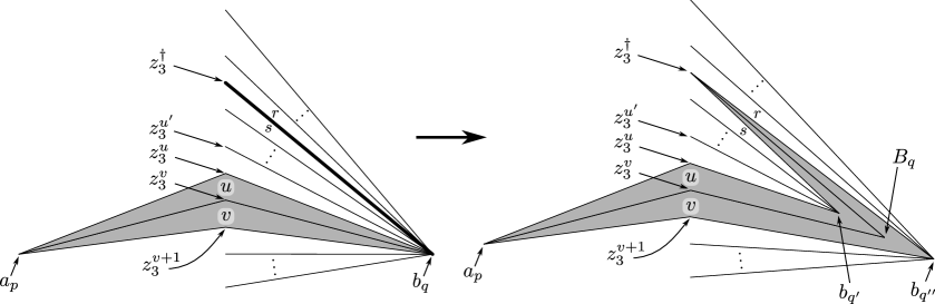
Figure 1: $wbp$-move: balloon’s head section is painted in gray, and the part of balloon’s tail that intersecting the appropriate semi-plane is depicted as a thick edge.

Figure 2: Given a half-wing and a balloon it can be partitioned into the balloon’s head section, thick edge and some almost triangulated sections.

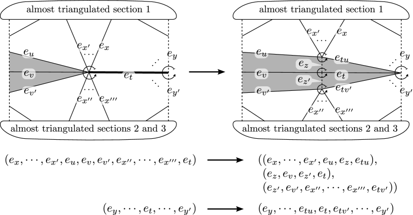
Figure 3: The star of a vertex of a graph embedded in a surface is the counterclockwise cyclic sequence of edges incident to the vertex (such an ordering is induced by the surface). The set of stars is called a rotation and has the characterizing property that each edge appears twice. The general case of changing rotation when going from $\mathcal{W}_{\ell-1}\cup\mathcal{N}_{\ell-1}$ to $\mathcal{W}_{\ell}\cup\mathcal{N}_{\ell}$ is depicted above. The rotation completely specifies the topological embedding.

A graph is rectilinearly embedded into $\mathbb{R}^{3}$ if the images of their edges are straight line segments. It is a straightforward application of Tutte’s barycentric method ([11], [1]) to obtain a rectilinear embedding of $\mathcal{W}_{n}^{h}\cup\mathcal{N}_{n}^{h}$ which fixes the vertices in the boundary of the outer triangular region of $\Pi_{h}$, $h\in\{\ell,r\}$. Tutte’s method has an intrinsic connection with the Laplacian of graphs, see [2]. We rotate $\Pi\in\{\Pi_{\ell},\Pi_{r}\}$ so that it becomes the $xz$-plane. After having the planar coordinates $\Pi_{h}$ is rotated back to its initial position and we have the $\mathcal{W}_{n}^{h}\cup\mathcal{N}_{n}^{h}$ rectilinearly embedded into $\mathbb{R}^{3}$. Tutte’s method becomes very efficient because of Lemma 1.2.

Tutte’s method suffers of the clustering problem where vertices accumulate in some small regions. Even though theoretically this is not needed, we present a heuristic of attaching weights to the edges to improve the result. An edge with weight $k\in\mathbb{N}$ behaves as $k$ parallel edges. We define the weights for the edges of the wings as 1. If the edge is in the nervure, to calculate the weight we use the whole wing. Start defining these weights as 0, so from leaves to root, define the weight of an edge as the weight of the vertex incident to it and closer to the leaves minus 1, Fig. 4. In Fig. 5 we compare the two results, without and with weights given by three times the weights in the nervure of Fig. 4, for obtaining the final left wing of the $r^{24}_{5}$-example.

Tutte’s method is applied twice: to plane graphs $\mathcal{W}_{n}^{\ell}\cup\mathcal{N}_{n}^{\ell}$ and to $\mathcal{W}_{n}^{r}\cup\mathcal{N}_{n}^{r}.$ In each application we use $O(n)$ iterations to solve a linear system in $\mathbb{C}$. This is theoretically sufficient to achive rectilineatiry (which nevertheless can be verified). As each one of the plane graphs has less than $6n-4$ edges by Lemma 1.2, the total time to obtain $\mathcal{W}_{n}^{\ell}\cup\mathcal{W}_{n}^{r}$ embedded into $\Pi_{\ell}\cup\Pi_{r}$ is $O(n^{2})$.

Lemma 1.2

The number of edges of $\mathcal{W}_{n}^{h}\cup\mathcal{N}_{n}^{h}$, $h\in\{\ell,r\}$ is at most $6n-4$.

Proof.    The number of 1-simplices in the left wing and in the right wing of the initial complex in the sequence are both $2n$. At each one of the $n-1$ $bp$-moves we add 4 edges either to the left or to the right wing with its nervure. Thus each one of the final left and right wings with nervures has at most $6n-4$ edges.

      □

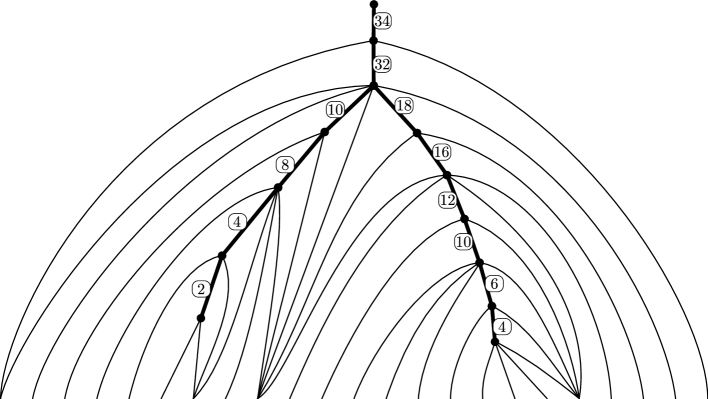
Figure 4: Computing the weights for Tutte’s barycentric method via the wing nervure.

Figure 5: Tutte’s embbeding without and with the weights (final pair of wings without nervure for the $r_{5}^{24}$-example).

1.2 Defining the PL-embedding $\mathcal{H}_{1}^{\diamond}$

Let $\mathcal{L}_{i+1}^{\star}$ be a subset of the pillow $\mathcal{P}_{i+1}^{\star}$, formed by the part that comes from the tail of the balloon after the i-th $bp$-move is applied, see Fig. 6.

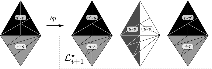
Figure 6: The set $\mathcal{L}_{i+1}^{\star}$.

Let $\{x\}\cup Y\subseteq\mathbb{R}^{N}$, for $1\leq N\in\mathbb{N}$. The cone ([10]) with vertex $x$ and base $Y$, denoted $x\ast Y\subseteq\mathbb{R}^{N}$, is the union of $Y$ with all line segments which link $x$ to $y\in Y$.

Now we define a PL-complex $\mathcal{H}^{\diamond}_{1}$ explicitly embedded into $\mathbb{R}^{3}$. We use the (rectilinearly embedded into $\Pi_{\ell}\cup\Pi_{r}$) final wings and the cone contruction to get the $\mathcal{H}^{\diamond}_{1}$. To this end, select a distinguished representative of the edges of $\mathcal{W}_{n}^{\ell}$ (resp. $\mathcal{W}_{n}^{r}$) incident to $z_{3}^{j}$ in the following way: if there is just one edge, choose it. Otherwise the representative is the edge whose other end has the smallest indexed upper case label. Let $R$ denote the set of representatives.

For each $e\in R$ add the two 2-simplices $z_{0}\ast e$ and $z_{2}\ast e$ (resp. the two 2-simplices $z_{1}\ast e$ and $z_{2}\ast e$) to $\mathcal{H}^{\diamond}_{1}$. To complete $\mathcal{H}^{\diamond}_{1}$ add the 2-simplices $\{z_{3}^{j}z_{1}z_{0}\ |\ j=1,\ldots,2n\}$. In Fig. 7 the solid lines (the edges of $R$) and the dashed edges are part of $\mathcal{L}^{\star}_{i}$, and are treated in next section.

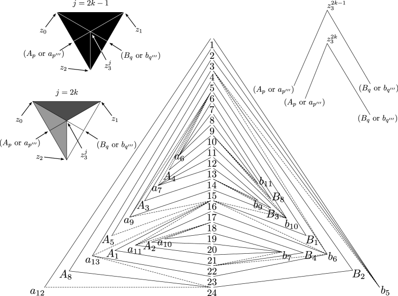
Figure 7: We use the cone construction with the solid lines to obtain $\mathcal{H}_{1}^{\diamond}.$ Then we use the dashed lines to obtain the information of $z_{3}^{\dagger}$ and $a_{p^{\prime}},A_{p},a_{p^{\prime\prime}}$ or $b_{q^{\prime}},B_{q},b_{q^{\prime\prime}}$ latter when obtaining $\mathcal{L}_{i}^{\star}$. Also, we have $p^{\prime\prime\prime}\in\{p^{\prime},p^{\prime\prime}\}$ and $q^{\prime\prime\prime}\in\{q^{\prime},q^{\prime\prime}\}$.

Proposition 1.3

If $\mathcal{W}_{m}^{h}$ is embedded rectilinearly in $\Pi_{h}$, $h\in\{\ell,r\}$, then the pair of embeddings can be extended to an embedding of $\mathcal{H}^{\diamond}_{1}$ into $\mathbb{R}^{3}$, via the cone construction.

Proof.    Straighforward from the simple geometry of the situation.

      □

1.3 Blowing up the tails and constructing
$\mathcal{H}_{2}^{\diamond},\mathcal{H}_{3}^{\diamond},\ldots,\mathcal{H}_{n}^{\diamond}=\mathcal{H}_{n}^{\star}$

The process of replacing the embedded tail of a balloon by the corresponding trio of PL2-faces in the pillow is denominated the blowing up of the balloon’s tail.

Theorem 1.4

There is an $O(n)$-algorithm for blowing up a single balloon’s tail. Thus finding $\mathcal{H}_{n}^{\star}$ and take $O(n^{2})$ steps.

Proof.    $\mathcal{H}_{i+1}^{\diamond}$ is the union of $\mathcal{H}_{i}^{\diamond}$ with $\mathcal{L}_{i+1}^{\star}$ and an $\epsilon$-change in some PL3-faces, if the rank of the type of balloon’s tail of the i-th $bp$-move has rank greater than 1 (we call $\epsilon$-change because this change is small, as described below). At the same time we update the colors of the middle layer to match the colors of the $i$-th pillow in the sequence of $bp$-moves.

Now we describe how to embed each kind of $\mathcal{L}_{i}^{\star}$ (explaining how to $\epsilon$-change some PL3-faces, to get space for $E\mathcal{L}_{i}^{\star}$).

If the balloon’s tail is of type $P_{1}$ (the case $B_{1}$ is analogous). Make two copies of $P_{1}$, resulting in three $P_{1}$, but change the color of the one which will be in the middle, and define the 0-simplices like in Fig. 8.

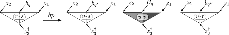
Figure 8: Embedding the part of the pillow corresponding to the tail of the balloon: case $P_{1}$ of the tail.

If the balloon’s tail is of type $B_{i}$, $i>1$ (the case $P_{i}$ is analogous). Make two copies of $B_{i}$, refine the copies and the original, resulting in three $B_{i}^{\prime}$, but change the color of the one which will be in the middle, and define the 0-simplices like in Fig. 9.

The images $\chi_{j}$ we already know from previous $bp$-move, now we need to define all the images $\alpha_{j},\beta_{j}$ and $\gamma_{j}.$ Let $\beta_{j}$ be $\frac{z_{2}+\chi_{j+1}}{2}$ for each $j=1,\ldots,i$. As the images $\alpha_{j}$ and $\gamma_{j}$ can be defined in analogus way, we just explain how to define each $\alpha_{j}$. We know that each $\alpha_{j}$ is in the PL3-face $\nabla_{r}$. To define each $\alpha_{j}$ we need to reduce the PL3-face $\nabla_{r}$ the get enough space for the PL2-faces of color 0 and 2 of the PL3-faces $\nabla_{u}$ and $\nabla_{v}$. Consider the PL3-face $\nabla_{r}$, each $\beta_{j}$ is already defined, so define each $\zeta_{j}$ as $\frac{z_{2}+\omega_{j+1}}{2}$, where $\omega_{k}$ is previously defined, see Fig. 10. Define $\alpha_{j}$ as $\frac{\zeta_{j}+\beta_{j}}{2}$.

Figure 9: Embedding the part of the pillow corresponding to the tail of the balloon: case $B_{i}$ of the tail.

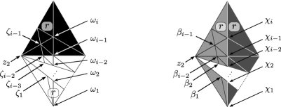
Figure 10: Using the PL3-face corresponding to $r$ to define the $\alpha_{j}$ as $\frac{\zeta_{j}+\beta_{j}}{2}$.

The last case is when balloon’s tail is refined, that means it is of type $P_{i}^{\prime}$ or $B_{i}^{\prime}$, $i>1$. We treat the case $B_{i}^{\prime}$, see Fig. 11. All the 0-simplices $\beta_{j}$ are already defined, we need to define each $\alpha_{j}$ and each $\gamma_{j}$. Observe that here $r\neq s-1$ and the definitions of $\alpha_{j}$ and $\gamma_{j}$ are not analogous.

Figure 11: Embedding the part of the pillow corresponding to the tail of the balloon: case $B_{i}^{\prime}$ of the tail.

In this case we need to reduce the PL3-faces $\nabla_{r}$ and $\nabla_{s}$ to create enough space to build PL2-faces 0- and 2-colored. To define 0-simplices $\alpha_{j}$ and $\gamma_{j}$, one of these cases is analogous to the case not refined, but the other we describe here ($\nabla_{r}$ is in the new case is the rank of PL2₀-face is equals to the rank of the PL2₁-face plus 2, if its not true, the new case is in the PL3-face $\nabla_{v}$). Suppose that the new case is in the PL3-face, $\nabla_{r}$. To define $\alpha_{j}$, suppose that the PL2₀-face of this PL3-face is not refined, see Fig. 12. Define each $\alpha_{j}$ as the middle point between $\beta_{j}$ and $\omega_{j}$.

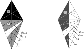
Figure 12: Using the PL3-face $\nabla_{r}$ to define $\alpha_{j}$ as $\frac{\omega_{j}+\beta_{j}}{2}$.

Consider the case that the PL2₀-face, of the PL3-face $\nabla_{r}$, is refined see Fig. 13. This is a final subtlety which is treated with the bump. This is characterized by a non-convex pentagon shown in the bottom part Fig. 13. Let $\nu_{j}$ be $\frac{z_{2}+\omega_{j}}{2}$ and $\alpha_{j}$ as $\frac{\beta_{j-1}+\nu_{j}}{2}$, for $j=1,\ldots,i-1$. Observe that if we define $\alpha_{j}$ as if the PL2₀-face where not refined, some 1-simplices may cross.

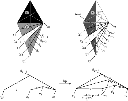
Figure 13: The bump: a final subtlety and how to deal with it.

      □

1.4 Obtaining the framed Link

Given $\mathcal{H}_{n}^{\star}$ into $\mathbb{R}^{3}$ we obtain the $k$-component framed link (corresponding to the $k$ twistors) as a set of PL-triangulated $k$ cylinders in the 2-skeleton of $\mathcal{H}_{n}^{\star}$, named $\mathcal{C}_{1},$ $\mathcal{C}_{2},\ldots,\mathcal{C}_{k}$. Observe that at this stage every 0-simplex of $\bigcup_{j=1}^{k}\mathcal{C}_{j}$ has a 3-D coordinate attached to it. These cylinders are parametrized as $k$ pairs of isometric rectangles (forming a strip) as in Fig. 14. We draw $k$ straight horizontal lines at different heights of the rectangles, in the example, lines $c_{1}-c_{1}$, $c_{2}-c_{2}$ and $c_{3}-c_{3}$. These lines are mapped into polygons in $\mathbb{R}^{3}$ which are PL-closed curves. The data we need is $\bigcup_{j=1}^{k}\mathcal{C}_{j}\subset\mathcal{H}_{n}^{\star}$ and we can discard the rest of $\mathcal{H}_{n}^{\star}$. The link that we seek is $\bigcup_{j=1}^{k}c_{j}$ with framing $\ell_{j}$, where $\ell_{j}$ is given by the linking number of the two components of $\mathcal{C}_{j}$ oriented in the same (arbitrary) direction. We briefly review the definition of linking number ([3]). Consider two distinct components $K_{1}$ and $K_{2}$ of an oriented link projected into the plane so that the crossings are transversal (no tangency) and that there are no triple points. The projection is also decorated in the sense that at each crossing the upper and the lower strands are given, usually, by omitting a small segment of the lower strand. The linking number of $\{K_{1},K_{2}\}$ is half of the algebraic sum of the signs of the crossings between $K_{1}$ and $K_{2}$, oriented in the same direction. If $G$ is a gem, $|G|$ means the 3-manifold induced by $G$. The link projection given in Fig. 15 which induce $|r^{24}_{5}|$ have its three linking numbers $-3$.

Proposition 1.5

The number of 1-simplices in $\bigcup_{j=1}^{k}c_{j}$ is at most $12n^{2}$, where $2n$ is the number of vertices of the input gem.

Proof.    A $c_{j}$ crosses one PL2_m-face, for $m\in\{0,1,2,3\}$. It is easy to verify that the maximum number of 2-simplices in $B_{i}^{\prime}$ or $P^{\prime}_{i}$ is $3i-1$ and this number exceeds similar numbers for $B_{i}$, $P_{i}$, $R^{b}_{i}$ and $R^{p}_{i}$, for $i\geq 1$. The maximum $i$ is $2n-1$, so the maximum number of 2-simplices 0-, 1- and 2-colored in one PL2-face of the final complex is $6n-4$. Each 1-simplex of $c_{j}$ crosses at most once each 2-simplex. Therefore, the number of 1-simpices crossing a 2-simplex 0-, 1- and 2-colored is at most $12n-8$. A $c_{j}$ crosses at most four 2-simplices 3-colored. The result follows because $n$ is an upper bound for $k$, number of components. Just note that a component in the link is in 1-1 correspondence with the twistors of the original gem and a twistor is formed by 2 vertices. This proof is partially ilustrated in Fig. 14. The illustration is not faithful because we can replace the strips at the right by their bottom parts, getting simpler cylinders homotopic to the ones illustrated.

      □

Each cylinder is formed by two strips. Each strip by two adequate pairs of two PL2-faces in the boundary of the PL3-faces in the hinge. In the way depicted we have one PL3-face of each color $c$, $c=0,1,2,3$. The number of crossings of the curves $c_{j}$, $j=1,2,3$ coincides with the number of $1$-simplices (or $0$-simplices) of $\bigcup_{j=1}^{3}\mathcal{C}_{j}$. To decrease this number we can replace the part of the strip which does not use a PL2₃-face by the two complementary PL2₃-faces in the corresponding PL3-face. This produces isotopic cylinders, but the number of crossings of the $c_{j}$’s are smaller. Note that each PL2₃-face has just five 2-simplices. In Fig. 14 we depict the situation for the wings arising from $r_{5}^{24}$ before the 3 replacements.

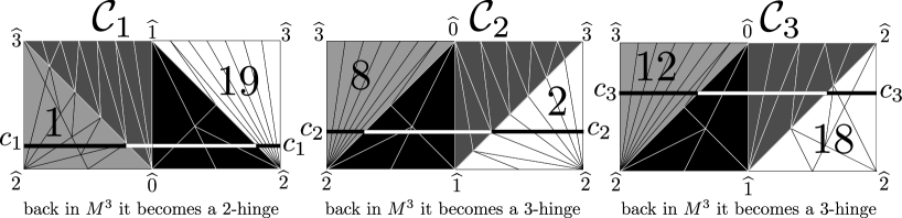
Figure 14: From hinges to cylinders $\mathcal{C}_{j}$ to curves $c_{j}$ (example inducing $|r^{24}_{5}|$).

Figure 15: Projection of the algorithm’s output, yielding the linking numbers of the boundary components of the embedded cylinders of Fig. 14.

1.5 Obtaining a Gauss code for the link

At this point, we have the link as a set of cyclic sequences of points in $\mathbb{R}^{3}$. We also have the framing of each component. Thus the theoretical problem is solved. However, is convenient to go on getting adequate planar projections to produce planar diagram for the link. We obtain the following Gauss code, ([9], chapter 3 of [5], [8]), where signs mean up $(+)$ and down $(-)$ passages: $((-2,+3,-4,+1),(-5,+6,+2,-1),$ $(-3,+4,-7,-6,+5,+7)).$ From this code we get the link planar diagram of Figs. 16. Since we have the framings curls can be removed. An explicit elegant framed link inducing the euclidean 3-manifold $|r^{24}_{5}|$ was previously unknown. We use Fig. 17 as input for L. Lins’s software [4] to obtain the WRT-invariants from $r=3$ to $r=20$ for the space $|r^{24}_{5}|$. We also apply our algorithm for the Weber-Seifert hyperbolic dodecahedron space, obtaining a link with 142 crossings, included in Appendix B.

Figure 16: Simplifying the link diagram for $|r_{5}^{24}|$.

Figure 17: Framed link, blackboard framed link and WRT-invariants for $|r_{5}^{24}|$. Data obtained from L. Lins software [4].

Algorithm 1.6

There exists an $O(n^{2})$-algorithm to produce, from a resoluble gem inducing an $M^{3}$, a blackboard framed link also inducing $M^{3}$.

Proof.    We start with a resoluble gem $G$ with $2n$ vertices. Here is the algorithm, justified by the theory previously developed:

• Form decreasing sequence of gems starting with $\mathcal{J}^{2}$, the $J^{2}$-gem associated with the resolution of $G$ performing adequate $0$- or $1$-flips and finishing at the bloboid $\mathcal{B}_{1}$: $\mathcal{J}^{2}=\mathcal{H}_{n},\mathcal{H}_{n-1},\ldots,\mathcal{H}_{1}=\mathcal{B}_{1}$.

• Form sequence of balloons $\mathcal{B}_{1}^{\star},\ldots,\mathcal{B}_{n-1}^{\star}$ and pillows $\mathcal{P}_{2}^{\star},\ldots,\mathcal{P}_{n}^{\star}$ defining implicitly the sequence of combinatorial $2$-complexes $\mathcal{H}_{1}^{\star},\mathcal{H}_{1}^{\star},\ldots,\mathcal{H}_{2n}^{\star}$, together with their respective wings and nervures (combinatorially given by rotations), $\mathcal{W}_{1}^{\ell}\cup\mathcal{N}_{1}^{\ell}$, $\mathcal{W}_{2}^{\ell}\cup\mathcal{N}_{2}^{\ell}$, …, $\mathcal{W}_{n}^{\ell}\cup\mathcal{N}_{n}^{\ell}$ and $\mathcal{W}_{1}^{r}\cup\mathcal{N}_{1}^{r}$, $\mathcal{W}_{2}^{r}\cup\mathcal{N}_{2}^{r}$, …, $\mathcal{W}_{n}^{r}\cup\mathcal{N}_{n}^{r}$. Each $bp$-move is simply a flip in the primal sequence. See Figs. 19 to 29 from the $r^{24}_{5}$-example.

• Use Tutte’s barycentric method with the edge weight heuristic (Fig. 4 from the $r^{24}_{5}$-example) to provide rectilinear embeddings of $\mathcal{W}_{n}^{\ell}\cup\mathcal{N}_{n}^{\ell}$ in $\Pi_{\ell}$ and of $\mathcal{W}_{n}^{r}\cup\mathcal{N}_{n}^{r}$ in $\Pi_{r}$ fixing the outer regions. The nervures are useful up to this point, and after obtaining the rectilinear embeddings they can be discarded.

• Get $\mathcal{H}_{1}^{\diamond}$ using $\mathcal{W}_{n}^{\ell}\cup\mathcal{W}_{n}^{r}$ by the cone construction.

• Get the sequence $\mathcal{H}_{2}^{\diamond},\ldots,\mathcal{H}_{n}^{\diamond}=\mathcal{H}_{n}^{\star}$ by the blowing up technique in the proof of Theorem 1.4.

• Define the framings of the components of the link as the linking numbers of the boundaries of the cylinders formed by the strips coming from the hinges; special care: distinguish the hinges which become 2-hinges from the hinges which become 3-hinges in $M^{3}$. See Fig. 14.

• Find an adequate projection of suitable medial curves in the cylinders. These curves form the link. Find Gauss code for the link, and so, a projection is combinatorially specified ([9], chapter 3 of [5], [8]). Add curls to produce a blackboard framed link. See Figs. 16 and 17 from the $r^{24}_{5}$-example.

This algorithm has both space complexity and time complexity $O(n^{2})$. Its output, first obtained as a set with no more than $n$ PL-polygons in $\mathbb{R}^{3}$, has a total of at most $12n^{2}$ vertices.

      □

———–

Appendix A: a solution for the Weber-Seifert Dodecahedral Hyperbolic Space

We found a projection for a framed link with 142 crossings for the Weber-Seifert Dodecahedral Hyperbolic Space. Actually the PL-link are nine PL-polygons in $\mathbb{R}^{3}$ with a total of only 68 vertices. The data that follows is a positive answer for Jeffrey Weeks’ question more than twenty years ago. Still in raw form, it can be substantially simplified

We apply our algorithm to the 50-vertex gem and its resolution given at the right side of Fig. 18.

Figure 18: This is a 50-vertex gem which behaves as the attractor.

A crossing $x\in\mathbb{N}$ has 4 legs in counterclockwise order: $(4x-3,4x-2,4x-1,4x)$. A duet is a perfect matching of the legs. The first entry of a quintet is the number of the crossing. Each crossing appears in two consecutive quintets. The second entry is $d$ or $u$ depending on whether the quintet holds the first or the second occurrence of its crossing. The $d$ means that the southwest to the northeast passage goes under, the $u$ means that it goes over. The third and fourth entries of a quintet are legs and their order specifies a consistent orientation for all the components of the link. The fifth and last entry of a quintet is the number of the component of the link that contains the two legs. By properly embedding the quintets in the plane and identifying the legs as specified by the duets we have a link diagram with consistent orientation of all of its component. Thus to obtain a Gauss code ([9], chapter 3 of [5], [8]), for the link is straightforward. Even though there are 142 crossings in the projection, the number of 1-simplices in the PL-link is only 68. This was obtained by a shortcutting technique which started with over two hundred 1-simplices: each 0-simplex defines a triangle in $\mathbb{R}^{3}$; if this triangle is not pierced by a 1-simplex, then the 0-simplex is removed from the link. Compare 68 with our theoretical bound, namely $12n^{2}=7500$, since $n=25$. We emphasize the issue that the algorithm behaves very efficiently.

1.6 Duets of $DHIP_{50}^{142}$

$\begin{array}[]{|c|c|c|c|c|c|c|c|}\hline\cr 1,8&2,155&3,112&4,111&5,108&6,11&7,104&9,16\\ 10,101&12,107&13,564&14,19&15,102&17,24&18,97&20,159\\ 21,158&22,27&23,468&25,32&26,465&28,163&29,340&30,35\\ 31,336&33,40&34,267&36,271&37,560&38,43&39,268&41,48\\ 42,75&44,559&45,72&46,51&47,76&49,56&50,495&52,71\\ 53,68&54,59&55,188&57,62&58,185&60,63&61,500&64,67\\ 65,70&66,183&69,184&73,494&74,79&77,84&78,263&80,259\\ 81,258&82,85&83,26&86,475&87,92&88,335&89,472&90,93\\ 91,466&94,471&95,98&96,467&99,156&100,103&105,110&106,319\\ 109,320&113,240&114,239&115,526&116,117&118,525&119,122&120,235\\ 121,236&123,142&124,127&125,132&126,531&128,139&129,136&130,135\\ 131,532&133,138&134,317&137,230&140,141&143,146&144,231&145,524\\ 147,528&148,149&150,527&151,154&152,383&153,244&157,164&160,563\\ 161,464&162,167&165,172&166,337&168,463&169,344&170,175&171,338\\ 173,180&174,269&176,275&177,556&178,181&179,558&182,497&186,191\\ 187,496&189,196&190,489&192,427&193,432&194,199&195,488&197,204\\ 198,435&200,431&201,448&202,207&203,544&205,212&206,443&208,447\\ 209,446&210,215&211,538&213,220&214,483&216,371&217,370&218,223\\ 219,376&221,226&222,373&224,311&225,522&227,316&228,229&232,523\\ 233,530&234,237&238,529&241,470&242,247&243,324&245,252&246,321\\ 248,327&249,326&250,253&251,568&254,329&255,260&256,479&257,332\\ 261,334&262,265&266,333&270,557&272,339&273,280&274,553&276,507\\ 277,506&278,283&279,416&281,288&282,413&284,411&285,552&286,291\\ 287,504&289,296&290,295&292,359&293,364&294,299&297,304&298,365\\ 300,363&301,452&302,305&303,366&306,451&307,312&308,369&309,396\\ 310,313&314,395&315,318&322,567&323,392&325,330&328,473&331,476\\ 341,404&342,347&343,408&345,352&346,511&348,403&349,516&350,353\\ 351,512&354,515&355,360&356,551&357,514&358,361&362,519&367,372\\ 368,445&374,379&375,484&377,382&378,535&380,521&381,536&384,387\\ 385,390&386,565&388,391&389,566&393,456&394,399&397,402&398,459\\ 400,455&401,460&405,510&406,409&407,508&410,549&412,505&414,503\\ 415,420&417,502&418,421&419,554&422,501&423,428&424,499&425,430\\ 426,429&433,440&434,485&436,543&437,542&438,441&439,546&442,541\\ 444,537&449,518&450,453&454,517&457,462&458,561&461,562&469,474\\ 477,482&478,533&480,539&481,534&486,545&487,490&491,548&492,493\\ 498,555&509,550&513,520&540,547&&&&\\ \hline\cr\end{array}$

1.7 Quintets, cylinders and framings of $DHIP_{50}^{142}$

$\begin{array}[]{cccccc}\{1,\text{d},3,1,1\}&\{1,\text{u},4,2,3\}&\{2,\text{d},7,5,8\}&\{2,\text{u},8,6,1\}&\{3,\text{d},11,9,1\}&\{3,\text{u},10,12,1\}\\ \{4,\text{d},13,15,8\}&\{4,\text{u},16,14,1\}&\{5,\text{d},18,20,2\}&\{5,\text{u},19,17,1\}&\{6,\text{d},24,22,1\}&\{6,\text{u},21,23,9\}\\ \{7,\text{d},27,25,1\}&\{7,\text{u},28,26,5\}&\{8,\text{d},32,30,1\}&\{8,\text{u},31,29,4\}&\{9,\text{d},35,33,1\}&\{9,\text{u},34,36,3\}\\ \{10,\text{d},39,37,9\}&\{10,\text{u},40,38,1\}&\{11,\text{d},42,44,8\}&\{11,\text{u},43,41,1\}&\{12,\text{d},48,46,1\}&\{12,\text{u},45,47,1\}\\ \{13,\text{d},51,49,1\}&\{13,\text{u},50,52,6\}&\{14,\text{d},53,55,2\}&\{14,\text{u},56,54,1\}&\{15,\text{d},59,57,1\}&\{15,\text{u},60,58,8\}\\ \{16,\text{d},61,63,8\}&\{16,\text{u},62,64,1\}&\{17,\text{d},66,68,2\}&\{17,\text{u},67,65,1\}&\{18,\text{d},70,72,1\}&\{18,\text{u},71,69,6\}\\ \{19,\text{d},73,75,8\}&\{19,\text{u},76,74,1\}&\{20,\text{d},80,78,4\}&\{20,\text{u},79,77,1\}&\{21,\text{d},84,82,1\}&\{21,\text{u},81,83,3\}\\ \{22,\text{d},86,88,9\}&\{22,\text{u},85,87,1\}&\{23,\text{d},91,89,9\}&\{23,\text{u},92,90,1\}&\{24,\text{d},93,95,1\}&\{24,\text{u},96,94,5\}\\ \{25,\text{d},99,97,2\}&\{25,\text{u},98,100,1\}&\{26,\text{d},102,104,8\}&\{26,\text{u},103,101,1\}&\{27,\text{d},108,106,8\}&\{27,\text{u},107,105,1\}\\ \{28,\text{d},109,111,3\}&\{28,\text{u},110,112,1\}&\{29,\text{d},115,113,6\}&\{29,\text{u},114,116,2\}&\{30,\text{d},120,118,8\}&\{30,\text{u},117,119,2\}\\ \{31,\text{d},123,121,2\}&\{31,\text{u},122,124,2\}&\{32,\text{d},126,128,6\}&\{32,\text{u},127,125,2\}&\{33,\text{d},129,131,8\}&\{33,\text{u},132,130,2\}\\ \{34,\text{d},135,133,2\}&\{34,\text{u},134,136,8\}&\{35,\text{d},138,140,2\}&\{35,\text{u},139,137,6\}&\{36,\text{d},141,143,2\}&\{36,\text{u},144,142,2\}\\ \{37,\text{d},146,148,2\}&\{37,\text{u},145,147,6\}&\{38,\text{d},149,151,2\}&\{38,\text{u},150,152,8\}&\{39,\text{d},154,156,2\}&\{39,\text{u},155,153,3\}\\ \{40,\text{d},159,157,2\}&\{40,\text{u},160,158,9\}&\{41,\text{d},164,162,2\}&\{41,\text{u},161,163,5\}&\{42,\text{d},167,165,2\}&\{42,\text{u},166,168,8\}\\ \{43,\text{d},172,170,2\}&\{43,\text{u},171,169,4\}&\{44,\text{d},175,173,2\}&\{44,\text{u},174,176,3\}&\{45,\text{d},179,177,9\}&\{45,\text{u},180,178,2\}\\ \{46,\text{d},181,183,2\}&\{46,\text{u},184,182,6\}&\{47,\text{d},188,186,2\}&\{47,\text{u},185,187,8\}&\{48,\text{d},192,190,7\}&\{48,\text{u},191,189,2\}\\ \{49,\text{d},196,194,2\}&\{49,\text{u},195,193,7\}&\{50,\text{d},200,198,5\}&\{50,\text{u},199,197,2\}&\{51,\text{d},204,202,2\}&\{51,\text{u},203,201,7\}\\ \{52,\text{d},207,205,2\}&\{52,\text{u},206,208,5\}&\{53,\text{d},209,211,7\}&\{53,\text{u},212,210,2\}&\{54,\text{d},214,216,8\}&\{54,\text{u},215,213,2\}\\ \{55,\text{d},217,219,4\}&\{55,\text{u},220,218,2\}&\{56,\text{d},222,224,5\}&\{56,\text{u},223,221,2\}&\{57,\text{d},226,228,2\}&\{57,\text{u},227,225,6\}\\ \{58,\text{d},230,232,6\}&\{58,\text{u},229,231,2\}&\{59,\text{d},233,235,8\}&\{59,\text{u},236,234,2\}&\{60,\text{d},237,239,2\}&\{60,\text{u},240,238,6\}\\ \{61,\text{d},244,242,3\}&\{61,\text{u},241,243,9\}&\{62,\text{d},247,245,3\}&\{62,\text{u},246,248,4\}&\{63,\text{d},251,249,9\}&\{63,\text{u},252,250,3\}\\ \{64,\text{d},253,255,3\}&\{64,\text{u},254,256,5\}&\{65,\text{d},257,259,4\}&\{65,\text{u},260,258,3\}&\{66,\text{d},263,261,4\}&\{66,\text{u},264,262,3\}\\ \{67,\text{d},266,268,9\}&\{67,\text{u},265,267,3\}&\{68,\text{d},270,272,8\}&\{68,\text{u},271,269,3\}&\{69,\text{d},276,274,8\}&\{69,\text{u},275,273,3\}\\ \{70,\text{d},279,277,6\}&\{70,\text{u},280,278,3\}&\{71,\text{d},284,282,5\}&\{71,\text{u},283,281,3\}&\{72,\text{d},287,285,9\}&\{72,\text{u},288,286,3\}\\ \{73,\text{d},292,290,6\}&\{73,\text{u},291,289,3\}&\{74,\text{d},296,294,3\}&\{74,\text{u},295,293,6\}&\{75,\text{d},299,297,3\}&\{75,\text{u},300,298,4\}\\ \{76,\text{d},304,302,3\}&\{76,\text{u},303,301,5\}&\{77,\text{d},305,307,3\}&\{77,\text{u},308,306,8\}&\{78,\text{d},312,310,3\}&\{78,\text{u},311,309,5\}\\ \{79,\text{d},313,315,3\}&\{79,\text{u},314,316,6\}&\{80,\text{d},319,317,8\}&\{80,\text{u},318,320,3\}&\{81,\text{d},324,322,9\}&\{81,\text{u},323,321,4\}\\ \{82,\text{d},326,328,9\}&\{82,\text{u},327,325,4\}&\{83,\text{d},330,332,4\}&\{83,\text{u},331,329,5\}&\{84,\text{d},335,333,9\}&\{84,\text{u},334,336,4\}\\ \{85,\text{d},339,337,8\}&\{85,\text{u},340,338,4\}&\{86,\text{d},344,342,4\}&\{86,\text{u},341,343,5\}&\{87,\text{d},347,345,4\}&\{87,\text{u},346,348,9\}\\ \{88,\text{d},351,349,6\}&\{88,\text{u},352,350,4\}&\{89,\text{d},353,355,4\}&\{89,\text{u},354,356,8\}&\{90,\text{d},357,359,6\}&\{90,\text{u},360,358,4\}\\ \{91,\text{d},364,362,6\}&\{91,\text{u},361,363,4\}&\{92,\text{d},365,367,4\}&\{92,\text{u},368,366,5\}&\{93,\text{d},372,370,4\}&\{93,\text{u},371,369,8\}\\ \{94,\text{d},376,374,4\}&\{94,\text{u},375,373,5\}&\{95,\text{d},379,377,4\}&\{95,\text{u},380,378,6\}&\{96,\text{d},382,384,4\}&\{96,\text{u},383,381,8\}\\ \{97,\text{d},387,385,4\}&\{97,\text{u},386,388,9\}&\{98,\text{d},391,389,9\}&\{98,\text{u},390,392,4\}&\{99,\text{d},393,395,6\}&\{99,\text{u},396,394,5\}\\ \{100,\text{d},399,397,5\}&\{100,\text{u},400,398,5\}&\{101,\text{d},403,401,9\}&\{101,\text{u},402,404,5\}&\{102,\text{d},407,405,6\}&\{102,\text{u},408,406,5\}\\ \{103,\text{d},410,412,8\}&\{103,\text{u},409,411,5\}&\{104,\text{d},414,416,6\}&\{104,\text{u},413,415,5\}&\{105,\text{d},419,417,9\}&\{105,\text{u},420,418,5\}\\ \{106,\text{d},421,423,5\}&\{106,\text{u},424,422,6\}&\{107,\text{d},425,427,7\}&\{107,\text{u},428,426,5\}&\{108,\text{d},429,431,5\}&\{108,\text{u},432,430,7\}\\ \{109,\text{d},435,433,5\}&\{109,\text{u},436,434,6\}&\{110,\text{d},439,437,7\}&\{110,\text{u},440,438,5\}&\{111,\text{d},441,443,5\}&\{111,\text{u},444,442,6\}\\ \{112,\text{d},448,446,7\}&\{112,\text{u},447,445,5\}&\{113,\text{d},451,449,8\}&\{113,\text{u},452,450,5\}&\{114,\text{d},454,456,6\}&\{114,\text{u},453,455,5\}\\ \{115,\text{d},460,458,9\}&\{115,\text{u},459,457,5\}&\{116,\text{d},463,461,8\}&\{116,\text{u},462,464,5\}&\{117,\text{d},468,466,9\}&\{117,\text{u},465,467,5\}\\ \{118,\text{d},472,470,9\}&\{118,\text{u},471,469,5\}&\{119,\text{d},473,475,9\}&\{119,\text{u},474,476,5\}&\{120,\text{d},479,477,5\}&\{120,\text{u},478,480,6\}\\ \{121,\text{d},482,484,5\}&\{121,\text{u},481,483,8\}&\{122,\text{d},486,488,7\}&\{122,\text{u},485,487,6\}&\{123,\text{d},489,491,7\}&\{123,\text{u},490,492,6\}\\ \{124,\text{d},496,494,8\}&\{124,\text{u},493,495,6\}&\{125,\text{d},498,500,8\}&\{125,\text{u},497,499,6\}&\{126,\text{d},501,503,6\}&\{126,\text{u},502,504,9\}\\ \{127,\text{d},506,508,6\}&\{127,\text{u},505,507,8\}&\{128,\text{d},510,512,6\}&\{128,\text{u},509,511,9\}&\{129,\text{d},516,514,6\}&\{129,\text{u},513,515,8\}\\ \{130,\text{d},519,517,6\}&\{130,\text{u},518,520,8\}&\{131,\text{d},523,521,6\}&\{131,\text{u},522,524,6\}&\{132,\text{d},525,527,8\}&\{132,\text{u},528,526,6\}\\ \{133,\text{d},532,530,8\}&\{133,\text{u},529,531,6\}&\{134,\text{d},536,534,8\}&\{134,\text{u},535,533,6\}&\{135,\text{d},538,540,7\}&\{135,\text{u},539,537,6\}\\ \{136,\text{d},542,544,7\}&\{136,\text{u},541,543,6\}&\{137,\text{d},548,546,7\}&\{137,\text{u},547,545,7\}&\{138,\text{d},551,549,8\}&\{138,\text{u},552,550,9\}\\ \{139,\text{d},556,554,9\}&\{139,\text{u},553,555,8\}&\{140,\text{d},560,558,9\}&\{140,\text{u},559,557,8\}&\{141,\text{d},562,564,8\}&\{141,\text{u},561,563,9\}\\ \{142,\text{d},566,568,9\}&\{142,\text{u},567,565,9\}&\end{array}$

Appendix B: all figures for the $r_{5}^{24}$-example. This produces an overview of the data structure and their interrelations illustrating the general case of the algorithm

In the following figures, the notation $\nabla_{v,i+1}$, $i\geq 1$, denotes the PL3-face dual of the vertex $v$ of the input gem obtained after the $i$-th $bp$-move is performed. If after the $i$-th $bp$-move $\nabla_{v,i}$ does not change, then $\nabla_{v,i+1}=\nabla_{v,i}$. When there is a change, it is an $\epsilon$-change.

References

- [1] É. Colin de Verdière, M. Pocchiola, and G. Vegter. Tutte’s barycenter method applied to isotopies. Computational Geometry, 26(1):81–97, 2003.
- [2] E Klarreich. Network solutions. Simons Foundation, April, 2012.
- [3] W.B.R. Lickorish. An introduction to knot theory, volume 175. Springer Verlag, 1997.
- [4] L.D. Lins. Blink: a language to view, recognize, classify and manipulate 3d-spaces. Arxiv preprint math/0702057, 2007.
- [5] S. Lins. Graphs of maps, Available in the arXiv as math.CO/0305058. PhD thesis, University of Waterloo, 1980.
- [6] S. Lins and R. Machado. Framed link presentations of 3-manifolds by an algorithm, I: gems and their duals. arXiv:1211.1953v2 [math.GT], 2012.
- [7] S. Lins and R. Machado. Framed link presentations of 3-manifolds by an algorithm, II: colored complexes and boundings in their complexity. arXiv:1212.0826v2 [math.GT], 2012.
- [8] S. Lins, E. Oliveira-Lima, and V. Silva. A homological solution for the Gauss code problem in arbitrary surfaces. Journal of Combinatorial Theory, Series B, 98(3):506–515, 2008.
- [9] P. Rosenstiehl. Solution algebrique du probleme de Gauss sur la permutation des points d’intersection d’une ou plusieurs courbes fermees du plan. CR Acad. Sci., 283:551–553, 1976.
- [10] C.P. Rourke and B.J. Sanderson. Introduction to piecewise-linear topology, volume 69. Springer-Verlag, 1982.
- [11] W.T. Tutte. How to draw a graph. Proc. London Math. Soc, 13(3):743–768, 1963.