The Markov Switching Multi-fractal models as a new class of REM-like models in 1-dimensional space.

Abstract

We map the Markov Switching Multi-fractal model (MSM) onto the Random Energy Model (REM). The MSM is, like the REM, an exactly solvable model in 1-d space with non-trivial correlation functions. According to our results, four different statistical physics phases are possible in random walks with multi-fractal behavior. We also introduce the continuous branching version of the model, calculate the moments and prove multiscaling behavior. Different phases have different multi-scaling properties.

I Introduction

The Random Energy Model (REM) introduced by Derrida de80 -de91 is one of the fundamental models of modern physics. Originally derived as a mean-field version of spin-glass models, it has subsequently been applied to describe some features of 2-d Liouville models ch96 ,ca97 , as well as the properties of quenched disorder in d-dimensional space with a logarithmic correlation function of energy disorder.

The logarithmic correlation is easy to organize both for models on a hierarchic tree and in 2-d. The REM structure in the d-dimensional logarithmic correlation case has been proved in ca01 using Bramson’s results br82 . In bu08 ,fy09 a REM-like model in 1-d space has been solved directly, using the generalization of Selberg integrals fy09 . A mapping has been used in sa09 to map the REM onto strings.

A REM can be formulated not only for the case of normal distributions of energies, which corresponds to the logarithmic correlation function of energies on a hierarchic tree, similar to logarithmic correlation functions in d-dimensional disorder case ca01 , but also for general distribution of energies de90 ,sa93 . It is an open problem to find solvable models with the non-logarithmic correlation for energy disorder in 1-d space. To describe the fluctuations in financial market, cf01 and cf02 have constructed some dynamical models, the Markov switching multi-fractal models (MSM). The MSM has time translational symmetry, contrary to cascade models, defined on hierarchic trees ca97 . The connection of the 1-d REM model fy09 with the multi-fractal random walk model ba00 -ba06 was found in sa11 . In this article we will prove that the dynamical models of cf01 and cf02 provide a 1-d REM where the correlation function for energies ($\ln u_{t}$ in our case) has a general character instead of being logarithmic.

Let us give the definition of the MSM model, following cf01 ; cf02 ; lu08 . In the MSM model, one considers the sequence of variables $r_{t}$, where $t\geq 0$ describes a discrete moment of time:

$$r_{t}=x_{t}u_{t},$$ (1)

$x_{t}$ has a normal distribution,

$$<x_{t}^{2}>=J^{2}$$ (2)

and $u_{t}$ is defined at the moment t of time via a product of k components $M(t,l)$

$$u_{t}=\prod_{l=1}^{k}M(t,l).$$ (3)

The variables $M(t,l)$ are random variables with some distribution.

Every moment of time our random variables are replaced with new ones with a probability

$$\gamma_{l}=1-\exp[-ab^{(l-k)}],$$ (4)

where $a>0,b>1,1\leq l\leq k$ are parameters of the model. The parameter $b$ plays the role of the branching number in cascade models (models of random variables on the branches of hierarchic models) and $k$ is the maximal number of hierarchy on the tree. An important difference is that now $b$ is a real number, while in case of hierarchic trees b should be an integer. Later we will formulate the continuous branching version of the model with a single relevant parameter $V$ defined from the equation

$$b^{k}=e^{V}\equiv L$$

$$b\to 1$$

$$L\to\infty$$ (5)

We will use the notation $L$ in sections II-H,III-B while investigating the multi-scaling properties of the model.

The model is named as ”random walk” model, because, due do Eq.(1), it is equivalent to the random walks with an amplitude $J^{2}$, when the time itself is a random variable see ba02 and sa11 for a simple proof. The random variables $M(t,l)$ are described via a Markov process, as any time period the transition probability depends only on the current state. There is a switching according to Eq.(4), thats why the authors of cf02 define it as a ”switching” model.

The distribution of $M(t,l)$ is chosen to ensure the constraint

$$<M(t,l)>=1,$$ (6)

where $<>$ means an average.

We can take the log-normal distribution for $M(t,l)$ or normal distribution for $\epsilon^{l}_{t}$, defined as

$$M(t,l)=\exp(\beta\epsilon^{l}_{t}),$$ (7)

where $\beta$ is similar to the inverse temperature in statistical physics.

We consider a distribution for $\epsilon$:

$$\rho(\epsilon)=\frac{\sqrt{k}}{\sqrt{2\pi V}}\exp[-\frac{k(\epsilon-\lambda)^{2}}{2V}],$$

$$\lambda=-\beta^{2}/2.$$ (8)

We have for $|t-t^{\prime}|<e^{V}$ the following two-point correlation function for $u_{t}$ :

$$<u_{t}u_{t^{\prime}}>\sim e^{\beta^{2}(2V-\ln|t-t^{\prime}|/\ln b)}.$$ (9)

The correlation function for $\ln u_{t},\ln u_{t^{\prime}}$ is logarithmic, as in models discussed in bu08 ,ca01 ,fy09 ,ba00 .

The previous expression is derived by observing that $u_{t}$ and $u_{t^{\prime}}$ have identical $M(t,l)$ for $\ln|t-t^{\prime}|/\ln b$ levels of hierarchy. The probability that $M(t,l)$ and $M(t^{\prime},l)$ are identical is

$$\sim\exp[-|t-t^{\prime}|e^{-ab^{(l-k)}}].$$ (10)

Thus $M(t,l)$ and $M(t^{\prime},l)$ are identical for l-th level of hierarchy defined through the inequality

$$k-\frac{\ln|t-t^{\prime}|}{\ln b}<l<k.$$ (11)

For the rest of the hierarchy levels $M(t,l)$ and $M(t^{\prime},l)$ are different.

When

$$\frac{\ln|t-t^{\prime}|}{V}\ll 1,$$ (12)

the majority of the hierarchies have the same $M(t,l)$ and $M(t^{\prime},l)$.

Alternatively, when

$$1-\frac{\ln|t-t^{\prime}|}{V}\ll 1,$$ (13)

$M(t,l)\neq M(t^{\prime},l)$ for the the majority of l.

In section III we derive some more rigorous results.

II The statistical physics of MSM

II.1 MSM with general distribution

Let us consider a general distribution for $\epsilon$

$$\rho_{0}(q,\epsilon)=\frac{1}{2\pi i}\int_{-i\infty}^{i\infty}dh\exp[-h\epsilon+q\phi(h)],$$ (14)

where $q$ is a parameter indicating some effective length.

We choose the distribution $\rho(\epsilon)$ with some shift

$$\rho(\epsilon)=\rho_{0}(\frac{V}{k},\epsilon-\lambda)$$ (15)

to ensure the constraint given by Eq. (6):

$$\int_{-\infty}^{\infty}d\epsilon\rho(\epsilon)\equiv e^{\beta\lambda+\frac{V}{k}\phi(\beta)}=1.$$ (16)

Thus we take

$$\lambda=-\frac{V\phi(\beta)}{\beta k}$$ (17)

where $k$ is our parameter describing the maximal hierarchy level. Hence, we have the following expression for the correlation function:

$$<u_{t}u_{t^{\prime}}>\sim e^{(V-\ln|t-t^{\prime}|/\ln b)\phi(2\beta)+2\phi(\beta)\ln|t-t^{\prime}|/\ln b}.$$ (18)

II.2 The statistical physics versus the dynamics

Let us define a partition function

$$z(i_{0},e^{V})=\sum_{i=i_{0}}^{i_{0}+e^{V}}x_{i}\prod_{l=1}^{k}M(i,l),$$ (19)

where $M(i,l)$ is chosen from the distribution given by Eq.(15).

Considering Eq.(1) as a dynamic process for a large period of time M, we define the probability distribution

$$P(z)=\frac{e^{V}}{M}\sum_{n=1}^{M/e^{V}}\delta_{z,z(1+e^{V}(n-1),e^{V}n)}.$$ (20)

We can define a statistical physics as well by considering $z$ as a partition function for the 1-d model with quenched disorder.

The average free energy, denoted as $<\ln Z>$ is:

$$<\ln Z>\equiv<\ln z(i_{0},e^{V})>.$$ (21)

Let us consider a related model with standard distribution for $\epsilon$ given by $\rho_{0}(\epsilon)$, without the constraint of Eq.(4).

We define

$$z_{0}(i_{0},e^{V})=\sum_{i=i_{0}}^{i_{0}+e^{V}}x_{i}\prod_{l=1}^{k}M(i,l),$$ (22)

where $M_{t}^{l}$ are defined through the distribution $\rho_{0}(\epsilon)$ and the corresponding free energy is

$$<\ln Z_{0}>\equiv<\ln z_{0}(i_{0},e^{V})>.$$ (23)

Eqs.(22) and (23) define a statistical physics model with $e^{V}$ configurations and special quenched disorder in 1-d space. Later we will focus on $<\ln Z>$.

It is easy to check that

$$<\ln Z>=<\ln Z_{0}>-V\phi(\beta).$$ (24)

Eq.(24) is an exact relation, correct for any value of $\beta$.

It is easier to solve the model for $<\ln Z_{0}>$. To calculate $<\ln Z_{0}>$, we will map the model onto the REM, and use the standard methods of REM. One can easily identify the most interesting transition in REM, from the high temperature phase to the SG phase, by just looking at the point in the high temperature phase where the entropy disappears.

We will calculate the partition function’s moments $<Z_{0}^{n}>$ and identify them with the $<Z_{REM}^{n}>$.

II.3 The moments in MSM model

First of all we calculate

$$<(Z_{0})^{2}>=e^{V}e^{V\phi(2\beta)}.$$ (25)

The cross terms vanishes due to integration by $x_{i}$.

Let us consider now

$$<(Z_{0})^{2n}>=\sum_{t_{1}}..\sum_{t_{2n}}<u_{t_{1}}..u_{t_{2n}}>.$$ (26)

While calculating the n-fold sum, we consider two principal contributions.

The first case is when all $t$ are close to each other and Eq.(12) is valid. There are $N_{1}\sim e^{V}$ such terms and the sum gives

$$\ln<(Z_{0})^{2n}>=V+V\phi(2n\beta)+O(1).$$ (27)

The second case corresponds to the integration from the regions where $t_{i+1}-t_{i}$ are of the same order, and therefore the condition given by Eq.(13) is satisfied. There are $N_{2}$ such terms,

$$\frac{\ln N_{2}-nV}{V}\ll 1.$$ (28)

As the vast majority of $M^{l}$ are different, the average gives

$$\ln<(Z_{0})^{2n}>=nV+nV\phi(2\beta)+O(1).$$ (29)

II.4 The corresponding REM

Consider now $e^{V}$ energy levels $E_{i}$ and define the partition function

$$Z_{REM}=\sum_{i=1}^{e^{V}}x_{i}e^{-\beta E_{i}},$$ (30)

where $-E_{i}$ have independent distributions by given Eq. (14) with $q=V$, and $x_{i}$ have normal distribution with variance 1.

The moments of the partition function for this model can be calculated exactly by following de89 and sa09 .

These moments are identical to the expressions given by Eqs. (27) and (29). We assume that two models with identical integer moments have an identical free energy as well.

The free energy of the REM model by Eq.(30) can be calculated rigorously following sa09 .

At high temperatures, we have the Fisher zeros (FZ) phase with

$$<\ln Z_{0}>=\frac{1}{2}\ln(Z_{0})^{2}=V\frac{\phi(2\beta)+1}{2}.$$ (31)

The transition point is at the point where the entropy disappears:

$$\beta_{c}\phi^{\prime}(2\beta_{c})=\frac{\phi(2\beta_{c})+1}{2}.$$ (32)

Below this temperature the system is in the SG phase with the free energy

$$V\beta\phi^{\prime}(2\beta_{c}).$$ (33)

Thus, we have found two phases. The phase given by Eq. (31) corresponds to the Fisher zero’s phase, while that given by Eq.(33) is the SG phase.

II.5 Asymmetric distribution

So far we have considered the case of a symmetric distribution of $x_{i}$. Let us now consider the asymmetric case described through the parameter $\gamma$, where

$$<u_{i}>=e^{-\gamma V}.$$ (34)

Now it is possible for the existence of a paramagnetic (PM) phase with the free energy

$$<\ln Z_{0}>=\ln<Z_{0}>=(-\gamma+1+\phi(\beta))V.$$ (35)

II.6 Large event

Let us assume that at the starting moment of time there is a large event described through the parameter A, while for the other times Eq.(2) is valid. We consider the following partition function

$$z_{0}(i_{0},e^{V})=-e^{AV}+\sum_{i=i_{0}+1}^{i_{0}+e^{V}}x_{i}\prod_{l=1}^{k}M(i,l).$$ (36)

Now we can have the fourth, ferromagnetic (FM), phase with

$$<\ln|Z_{0}|>=\ln<Z_{0}>=AV.$$ (37)

Actually we can consider an infinite series of time, when after $e^{V}$ there is a member $r_{i}=-e^{AV}$, while for other moments of time we calculate $r_{t}$ according to Eqs.(1) and (3).

II.7 Transition points

We should choose the proper phase by comparing the expressions given by Eqs. (31),(33),(35), (37) and then selecting the one which gives the maximum.

For example, the system transforms from the FZ phase to the PM phase at

$$e^{(1-\gamma+\phi(\beta))V}>J^{2}e^{\frac{V}{2}(1+\phi(2\beta))},$$ (38)

where $J^{2}$ is the variance of $x_{t}$ given by Eq.(2).

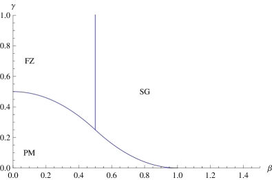
Figure 1: The phase structure of the model with asymmetric distribution of weights. The case of normal distribution $\phi(\beta)=\beta^{2}$.

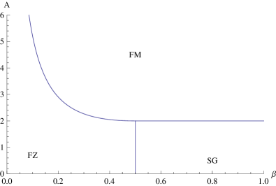
Figure 2: The phase structure of the model with a large event. The case of normal distribution $\phi(\beta)=\beta^{2}$.

In Figs. 1,2 we compare the numerics with our analytical results for the free energy.

II.8 The scale dependence of the free energy

Consider again the average distribution of Z, except that, instead of considering the sum over $e^{V}$ terms as in Eq.(20), consider the sum over $l\equiv e^{\alpha V}$ terms,

$$P(z)=\frac{l}{M}\sum_{n=1}^{M/l}\delta_{z,z(\alpha,1+l(n-1),ln)},$$ (39)

where $\epsilon$ have the distribution by Eq.(14). At high temperatures we have Fisher zeros (FZ) phase with

$$<\ln Z_{0}>=V\frac{\phi(2\beta)+\alpha}{2}$$ (40)

and for the critical point:

$$\beta_{c}\phi^{\prime}(2\beta_{c})=\frac{\phi(2\beta_{c})+\alpha}{2}.$$ (41)

As $\alpha<1$, the $\beta_{c}$ decreases with the decrease of $\alpha$.

III The case of continuous branching

III.1 The calculation of moments.

All the formulae in the previous sections have been derived for the case of general values of b. Consider the case:

$$a=1,k=\frac{V}{\delta v},b=1+\delta v,$$

$$\delta v\to 0$$ (42)

and the random variables are distributed according $\rho_{0}(\delta v,\epsilon)$.

The the i-th level of hierarchy is unchanged during the period of time $t$ with a probability:

$$\exp[-te^{v-V}],$$

$$v=i\delta v.$$ (43)

Multiplying the probabilities in Eq.(43) for different levels of hierarchy, we obtain

$$<u_{t_{1}}u_{t_{2}}>=$$

$$\prod_{i=1}^{k}[(1-\exp(-te^{v}))e^{\delta v2\phi(\beta)}+\exp(-te^{v})e^{\delta v\phi(2\beta)}]=$$

$$\exp[\sum_{i}\ln((1-\exp(-te^{v}))e^{\delta v2\phi(\beta)}+\exp(-te^{v})e^{\delta v\phi(2\beta)})]$$ (44)

Replacing the product by an integral and introducing variables $x_{i}=t_{i}/e^{V}$, we derive

$$\int_{0}^{e^{V}}dt_{1}dt_{2}<u_{t_{1}}u_{t_{2}}>=$$

$$e^{V(2(1+\phi(\beta)))}\int_{0}^{1}dx_{1}dx_{2}\exp[\int_{0}^{V}dv[\Phi_{2}(e^{v},x_{1},x_{2})]$$

$$\Phi_{2}(e^{v},x_{1},x_{2})=e^{-|x_{2}-x_{1}|e^{v}}(\phi(2\beta)-2\phi(\beta))$$ (45)

We get an asymptotic expression with the $e^{-V}$ accuracy in the limit $V\to\infty$:

$$\frac{\int_{0}^{e^{V}}dt_{1}dt_{2}<u_{t_{1}}u_{t_{2}}>}{e^{2V+2V\phi(\beta)}}=$$

$$\int_{0}^{1}dx_{1}dx_{2}e^{\int_{0}^{\infty}dv\Phi_{2}(e^{v},x_{1},x_{2})}.$$ (46)

Similarly, we derive the expression for the multiple correlations:

$$\frac{\int_{0}^{e^{V}}dt_{1}..t_{n}<u_{t_{1}}..u_{t_{n}}>}{e^{nV+n\phi(\beta)}}=$$

$$\int_{0}^{1}dx_{1}..dx_{n}e^{\int_{0}^{\infty}dv\Phi_{n}(e^{v},x_{1}..x_{n})}.$$ (47)

The latter expression is $O(1)$, as has been assumed before in Eq. (29).

For the 3-point correlation function we obtain

$$\Phi_{3}(y,x_{1},x_{2},x_{3})=3+3\phi(\beta)+$$

$$e^{-(x_{12}+x_{23})y}(\phi(3\beta)-3\phi(\beta))$$

$$+e^{-x_{12}y}(1-e^{-x_{23}y})(\phi(2\beta)-2\phi(\beta))$$

$$+(1-e^{-x_{12}y})e^{-x_{23}y}(\phi(2\beta)-2\phi(\beta))]$$ (48)

where we denote $x_{12}=|x_{1}-x_{2}|,x_{23}=|x_{2}-x_{3}|$. For n-point correlation function we need to consider $2^{n-1}$ terms in the expression of $\Phi_{n}$.

We can identified this terms with different paths on a tree with branching number 2, the jumps to the right give a coefficient $F(x,1)$ and $F(x,-1)$ for the left jump:

$$F(x,1)=\exp[-xe^{v}],F(x,-1)=(1-\exp[-xe^{v}])$$ (49)

The path is fractured into clusters, when we have l subsequent right jumps. We define

$$f_{l}=\phi(l\beta)$$ (50)

We should consider all the paths, the identify the n clusters of the given path with the length $l_{m}$ for the m-th cluster. Then we calculate

$$\Phi_{n}(e^{v},x_{1}...x_{n})=$$

$$\sum_{paths}[\prod_{i=0}^{n-1}F(x_{i,i+1,\alpha})](\sum_{m}f_{l_{m}}-n\phi(\beta))$$ (51)

III.2 Multi-scaling

If we consider the model for $l=e^{\alpha V}$ period of time and a normal distribution, we have in the high temperature phase

$$F\equiv\frac{<\ln Z_{0}>}{\alpha V}=\frac{1}{2}+\frac{\beta^{2}}{\alpha}$$ (52)

and in the SG phase

$$F\equiv\frac{<\ln Z_{0}>}{\alpha V}=\beta\sqrt{2/\alpha}.$$ (53)

The transition point is at

$$\beta_{c}=\sqrt{\alpha/2}.$$ (54)

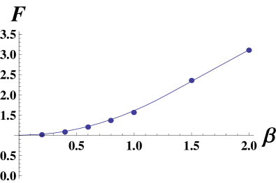
Figure 3: Free energy F versus an inverse temperature $\beta$ for the continuous branching model given by Eq.(42) and a normal distribution. The analytical results by Eqs.(52),(53), $V=14,N=100000$ are given by smooth lines.

In Fig.3 we compare the numerics with our analytical results for the free energy.

Let us calculate the multi-fractal properties of the MSM. We need to calculate the moments of the partition function

$$\int_{0}^{l}dt_{1}...dt_{n}<u_{t_{1}}...u_{t_{n}}e^{-n\phi(\beta)V}>\equiv e^{\ln\frac{l}{L}\xi(n,\beta)}A(L)^{n}C_{n},$$ (55)

where $\xi(n,\beta)$ defines the multi-scaling, $A(L)$ is some large numbers while $C_{n}\sim O(1)$.

While calculating the moments, we slightly modify the formulae of the previous sections. Instead of Eq.(46) now we obtain

$$\int dt_{1}..dt_{n}u(t_{1})...u(t_{n})=\int dx_{1}..dx_{n}\times$$

$$\exp[nV(1+\phi(\beta))+\int_{0}^{\infty}dv\Phi_{n}(\frac{l}{L}e^{v},x_{1}...x_{n})].$$ (56)

We consider the case $1\ll l\ll L$. Then, using the equation

$$\Phi_{n}(0,x_{1}...x_{n})=n\phi(\beta)-\phi(n\beta),$$ (57)

we derive, integrating by parts:

$$\int_{1}^{\infty}\frac{dy}{y}\Phi_{n}(y\frac{l}{L},x_{1}...x_{n})=$$

$$=(\phi(n\beta)-n\phi(\beta))\ln\frac{l}{L}-\int_{0}^{\infty}dy\ln y\Phi_{n}^{\prime}(y,x_{1}...x_{n}).$$ (58)

Thus we get a multi-scaling with

$$\xi(n,\beta)=n+n\phi(\beta)-\phi(n\beta).$$ (59)

Considering the moments of

$$z=\sum_{t=1}^{l}u_{t},$$ (60)

where for $u_{t}$ we use the distribution given by Eq.(15), we obtain

$$\frac{<z^{n}>}{L^{n}n!}=e^{\xi(n,\beta)\ln\frac{l}{L}}\int_{0}^{1}dx_{1}...dx_{n}e^{-\int_{0}^{\infty}dy\ln y\Phi_{n}^{\prime}(y,x_{1}...x_{n})}$$ (61)

and here $x_{1}...x_{n}$ are time ordered.

III.3 The moments for the model with random Boltzman weights.

Let us calculate now the moments $<z^{n}>$ for

$$z=\sum_{t=1}^{l}x_{t}u_{t}.$$ (62)

Using Eq.(8) from sa11 , we derive

$$\frac{<z^{2n}>}{(LJ)^{n}}=\frac{2^{n}\Gamma(\frac{1+2n}{2})}{\sqrt{\pi}}(\frac{l}{L})^{\xi(n,2\beta)}$$

$$n!\int_{0}^{0}dx_{1}...dx_{n}\exp[-\int_{0}^{\infty}dy\ln y\Phi_{n}^{\prime}(y,2\beta,x_{1}...x_{n})],$$ (63)

where there is a time ordering $t_{1}<t_{2}<..t_{n}$.

III.4 The multiscaling properties of different phases

There are no simple order parameters to distinguish the FZ and SG phases. If we enlarge the free energy expression to the complex temperatures $\beta=\beta_{1}+i\beta_{2}$, then in FZ phase there is a finite density $\bar{\rho}$ of partition function zeros, defined trough the formula de91a :

$$\bar{\rho}(\beta_{1},\beta_{2})=\frac{1}{2\pi}\frac{<\ln z(\beta_{1},\beta_{2})>}{V},$$ (64)

while in the SG phase this density is zero.

SG and FZ phases have different schemes of replica symmetry(breaking) sa01 .

There is a slow relaxation in THE SG phase. Unfortunately there are no any results about the dynamics of FZ phase to compare.

More interesting is to distinguish two phases looking the multiscaling properties. We investigated well the muultiscaling properties of FZ phase. Let us investigate now the SG phase.

Here there are the results by Gardner and Derrida de89 about the the moments of partition functions and the probability distribution.

Consider again the model with $z=\exp[\alpha V]$ configurations. For the case

$$\beta>\beta_{c}\sqrt{\alpha},\beta_{c}\sqrt{\alpha}>n\beta$$ (65)

we have, rescaling the result of de89 ,

$$\ln<z^{n}(\alpha)>=n\beta V\sqrt{\alpha}$$ (66)

In case of the multiscaling the right hand side is proportional to $\alpha$.

Thus there is a lack of any scaling in the SG phase and we can distinguish the SG and FZ phases checking the multiscaling property. We can distinguish FZ and SG phases also looking the tails of the distributions.

For the FZ phase a simple rescaling of the results of fy09 gives for the large $z$:

$$P(z)\sim\frac{1}{z^{1+\frac{\alpha\beta_{c}^{2}}{2\beta^{2}}}}$$ (67)

while in the SG phase we used the rescaled result by de89

$$P(z)\sim\frac{1}{z^{1+\frac{\sqrt{\alpha}\beta_{c}}{\beta}}}$$ (68)

where $\beta_{c}/\sqrt{2}$ is the transition point at $\alpha=1$. Eq.(68) is the result for the REM. For the logarithmic REM a more accurate expression includes a multiply $\ln{Z}$ on the right hand side of Eq.(68) fy12 .

IV The dynamic model

Let us return to the dynamic model given by Eq.(1). Mapping

$$e^{-\gamma V}=\mu\delta t,\quad J^{2}=\sigma^{2}dt,$$ (69)

we identify this version of the model at $\beta=0$ as a finite time version of driven Brownian motion de02 . In case of simple random walks with $\beta=0$, there is a single phase. In the model given by Eq.(1) with $\beta\neq 0$ we have an intrinsic large parameter $L\equiv e^{V}$, describing the effective number of configurations in the model. In this way the statistical physics enters into the dynamical problem. Contrary to the driven Brownian motion and the Heston model he , we have 4 different phases in the MSM model. The same is the situation with other models of multi-scaling random walks ba00 .

To identify the choice amongst the two phases (FZ versus PM) we consider

$$C=\frac{\sigma}{|\mu|\sqrt{T}}.$$ (70)

When $C\ll 1$, the system is in the PM phase. Otherwise at $C\gg 1$ we have the FZ phase.

V Conclusion

We considered the dynamic Markov switching multi-fractal models (MSM) and connected them with a new class of solvable statistical physics models of quenched disorder in one dimension. In these models there is both translational invariance and general distribution of disorder. While the multiscaling in FZ phase has been investigated before, nor the statistical physics properties properties, neither the phase structure has been investigated before. We found the exact phase structure of the model. At different phases there should be different distributions $P(z)$. In case of a symmetric random walk there are two phases in the considered model. At small parameters $\beta$, the model is in the phase with non-zero density of Fisher’s zeros. At high $\beta$, the system is in the spin-glass phase, a pathologic phase with a slow relaxation dynamics. For an asymmetric distribution of $x_{i}$ there is a possibility for the third, paramagnetic, phase. Slight modification of the model allows the existence of the fourth, ferromagnetic, phase. It is possible to distinguish different phases measuring the multi-scaling properties of the model. The multi-scaling is broken in the SG phase. We also introduced a continuous hierarchy branching version of the MSM, gave expressions for the moments of the partition function, and calculated the multi-scaling indices.

For applications it is important to calculate the fractional moments of the partition function. Perhaps we can use expressions for integer moments and use some approximate methods of extrapolation. Another interesting open problem is to investigate the dynamics of the model, looking for a new phase transition point in the dynamics, as is the case of the spherical spin-glass model cr93 .

DBS thanks Academia Sinica for financial support, Y. Fyodorov, S. Jain, Th. Lux, D. Sornette and O. Rozanova for discussions.

References

• (1) B. Derrida, Phys. Rev. Lett. 45, 79(1980) , Phys. Rev.B. 24, 2613(1981).
• (2) Derrida B. and Spohn H., J. Stat. Phys., 51, 817(1988).
• (3) E. Gardner, B. Derrida, J. Phys. A22, 1975 (1989).
• (4) J. Cook and B. Derrida, J. Stat. Phys., 61, 961 (1990).
• (5) J. Cook and B. Derrida, J. Stat. Phys., 63, 505 (1991).
• (6) C. C. Chamon, C. Mudry, X. G. Wen, Phys. Rev. Lett., 77 (1996) 4194.
• (7) H. E. Castillo, C. C. Chamon, E. Fradkin, P. M Goldbart, C. Mudry, Phys. Rev. B., 56, 10668 (1997).
• (8) D. Carpentier, P. Le Doussal, Phys. Rev. E, 63, 026110 (2001).
• (9) Bramson M., Mem. Am. Math. Soc., 44, 285 (1983).
• (10) Y. V. Fyodorov and J. P. Bouchaud, J. Phys. A 41 372001 (2008).
• (11) Y. V. Fyodorov ,P. Le Doussal, and A. Rosso, J. Stat. Mech. (2009) P10005.
• (12) D.B. Saakian, JSTAT (2009) P07003.
• (13) D.B. Saakian, Phy. Lett. 180A, 169 (1993).
• (14) L. Calvet, A. Fisher, Econometrics 105, 27 (2001).
• (15) L. Calvet and A. Fisher, Review of Economics and Statistics 84, 381 (2002).
• (16) J. F. Muzy, J. Delour and E. Bacry, Eur. Phys. J. B 17 537 (2000).
• (17) J. F. Muzy, E. Bacry, Phys. Rev. E 66056121 (2002).
• (18) J. F. Muzy, E. Bacry, and A. Kozhemyak Phys. Rev. E 73 066114 (2006).
• (19) D. B. Saakian, A. Martirosyan, C-K. Hu, Z. Struzik, EPL 95, 28007 (2011).
• (20) R. Liu, T. Di Matteo,T. Lux, Advances in Complex Systems, 11,669 (2008).
• (21) B. B. Mandelbrot, L. Calvet, and A. Fisher (1997), preprint, Cowles Foundation Discussion paper 1164.
• (22) Y. Fyodorov, Private information.
• (23) B. Derrida, Physica A 177,31 (1991).
• (24) D.B. Saakian, arXiv:cond-mat/0111251
• (25) E. Derman, Quantitative Finance 2, 282 (2002).
• (26) S. L. Heston, Journal of The Review of Financial Studies,6, 327 (1993).
• (27) A. Crisanti, H. Horner, and H.-J. Sommers, Z. Phys. B 92, 257(1993).