Work fluctuations for a Brownian particle in a harmonic trap with fluctuating locations

Abstract

We consider a Brownian particle in a harmonic trap. The location of the trap is modulated according to an Ornstein-Uhlenbeck process. We investigate the fluctuation of the work done by the modulated trap on the Brownian particle in a given time interval in the steady state. We compute the large deviation as well as the complete asymptotic form of the probability density function of the work done. The theoretical asymptotic forms of the probability density function are in very good agreement with the numerics. We also discuss the validity of the fluctuation theorem for this system.

I Introduction

Equilibrium statistical mechanics provides us a well-established framework to deal with systems in thermal equilibrium. When a system is perturbed externally from its equilibrium state, the so-called fluctuation-dissipation theorem relates the linear response of the system (to the external perturbation) to the fluctuations properties of the system in equilibrium (in the absence of the perturbation) Kubo:1966 . Within the framework of linear response theory, the Green-Kubo relation gives linear transport coefficients in terms of integral over time-correlation function of the corresponding current in equilibrium Green-Kubo . In contrast, a general understanding of nonequilibrium (arbitrarily far from equilibrium) systems is rather poor. That is why there has been a lot of excitement surrounding the fluctuation theorem, which aims at making a general statement about the fluctuations of entropy production during a nonequilibrium process. The fluctuation theorem has been suggested as a natural extension of the fluctuation-dissipation theorem from the linear response regime to arbitrarily far from equilibrium, as the fluctuation theorem reduces to the Green-Kubo formula and the Onsager reciprocity relations in the zero forcing limit Gallavotti:96 .

Imagine, two heat reservoirs at different temperatures connected by a thermal conductor. For a macroscopic object, we expect the heat to flow across the conductor from the hotter to the colder reservoir, in accordance with the second law of thermodynamics. However, for small systems, where microscopic fluctuations become important, once in a while we might observe heat to flow from the colder to the hotter reservoir. These reverse events are usually referred to as “second law violation”. The fluctuation theorem gives a mathematical expression for the ratio of the probability of “obeying the second law” to that of the “second law violation”.

Following a theoretical argument, Evans et. al. found a relation between the probabilities of positive and negative entropy production in the nonequilibrium steady state, in a molecular dynamics simulation of a two-dimensional fluid driven by external shear and coupled to a thermostat Evans:93 . Gallavotti and Cohen proved this relation (and called it fluctuation theorem) for the phase space contraction (interpreted as the entropy production) for dissipative dynamical systems in the nonequilibrium steady-state using chaotic hypothesis and time reversal invariance Gallavotti:95 . Evans and Searles had derived earlier a similar relation (now known as the transient fluctuation theorem) for systems starting from equilibrium initial condition Evans:94 . For stochastic systems, the fluctuation theorem has been proven by Kurchan Kurchan:98 for Langevin dynamics and extended by Lebowitz and Spohn Lebowitz:99 to general Markov processes. Subsequently, there has been an explosion of research activities investigating the validity of the fluctuation theorem for other quantities such as work, power flux, heat flow, total entropy, etc., both theoretically Farago:02 ; vanZon:03 ; vanZon:04 ; Mazonka:99 ; Narayan:04 ; Bodineau:04 ; Seifert:05 ; Baiesi:06 ; Bonetto:06 ; Visco:06 ; Mai:07 ; Saito:07 ; Harris:07 ; Kundu:11 ; Saito:11 ; Sabhapandit:11-12 ; Fogedby:11 ; Kundu:12 and experimentally Wang:02 ; Wang:05 ; Carberry:04 ; Goldburg:01 ; Feitosa:04 ; Garnier:05 ; Liphardt:02 ; Collin:05 ; Majumdar:08 ; Douarche:06 ; Falcon:08 ; Bonaldi:09 ; Ciliberto:10 ; Ciliberto:10-2 ; Gomez-Solano:11 . The recent review Seifert:2012 contains an extensive list of references pointing to several other reviews as well as research articles on fluctuation theorem and related topics.

Recently, Ref. Ciliberto:10 reported experiments on the fluctuations of the work done by an external Gaussian random force on two different stochastic systems coupled to a thermal bath: (i) a colloidal particle in an optical trap and (ii) an atomic-force microscopy cantilever. Analytical results have been obtained for the second system in Sabhapandit:11-12 . In the first experiment, a colloidal particle immersed in water (which acts as thermal bath) is confined in an optical trap. The position of the trap is modulated according to a Gaussian Ornstein-Uhlenbeck process. The authors have experimentally determined the probability density function (PDF) of the work done on the colloidal particle by the random force exerted by the modulating trap. In this paper, we analytically treat this problem.

The remainder of the paper is organized as follows. In Sec. II, we define the model. Section III contains the derivation of the moment generating function of work done $W_{\tau}$ in a given time $\tau$, which has the form $\bigl{\langle}e^{-\lambda W_{\tau}}\bigr{\rangle}\approx g(\lambda)\,e^{\tau\mu(\lambda)}$ for large $\tau$. In Sec. IV, we invert the moment generating function to obtain the asymptotic form (for large $\tau$) of the PDF of $W_{\tau}$. We find that in that relevant interval, $g(\lambda)$ can either be analytic, or can have either one branch point or three or four branch points, depending on the values of the tuning parameters of the problem. The case when $g(\lambda)$ is analytic, is simpler and the asymptotic PDF can be obtained by the usual saddle point approximation, which is given by Eq. (27) in Sec. IV.1. In Sec. IV.2, we deal with case when $g(\lambda)$ has one branch point. The cases when $g(\lambda)$ has three and four branch points are discussed in Secs. IV.3 and IV.4, respectively. The analytical results obtained in each section are supported by numerical simulation performed on the system. Section V contains a discussion on large deviation function and validity of the fluctuation theorem in the context of the problem at hand. Finally, we summarize the paper in Sec. VI. Some details of calculation are pushed to two appendices: Appendix A contains the details of the calculation of the moment generating function. In Appendix B, we analyze the singularities of $g(\lambda)$ and in Appendix C we give the steepest descent method with branch point to calculate the PDF. We also provide an index of the relevant notations used in the paper in Appendix D, for the ease of quick look up.

II The model

Consider a Brownian particle suspended in a fluid at temperature $T$, with the viscous drag coefficient $\gamma$. The particle is confined in a quadratic potential (harmonic trap) around the position $y$ and having a stiffness $k$. The position $x(t)$ of the particle is described by the overdamped Langevin equation

$$\frac{dx}{dt}=-\frac{x-y}{\tau_{\gamma}}+\xi(t),$$ (1)

where $\tau_{\gamma}=\gamma/k$ is the relaxation time of the harmonic trap. The thermal noise $\xi(t)$ is taken to be Gaussian with mean $\langle\xi(t)\rangle=0$ and covariance $\langle\xi(t)\xi(s)\rangle=2D\delta(t-s)$, where the diffusion coefficient $D=\gamma^{-1}k_{B}T$ with $k_{B}$ being the Boltzmann constant. An external time-varying random force is exerted by the trap on the Brownian particle by externally modulating the position of the trap according to an Ornstein-Uhlenbeck process

$$\frac{dy}{dt}=-\frac{y}{\tau_{0}}+\zeta(t),$$ (2)

where $\zeta(t)$ is an externally generated Gaussian white (non-thermal) noise with mean $\langle\zeta(t)\rangle=0$ and covariance $\langle\zeta(t)\zeta(s)\rangle=2A\delta(t-s)$. There is no correlation between the externally applied noise and the thermal noise, $\langle\zeta(t)\xi(s)\rangle=0$. The system eventually reaches steady state, and in the steady state the trap exerts a correlated random force $ky(t)$ on the Brownian particle with mean $\langle y(t)\rangle=0$ and covariance $\langle y(t)y(s)\rangle=A\tau_{0}\exp(-|t-s|/\tau_{0})$. The quantity of our interest is the work done in the steady state, by the random force exerted by the trap on the Brownian particle in a given time duration $\tau$. This is given (in units of $k_{B}T$) by

$$W_{\tau}=\frac{1}{k_{B}T}\int_{0}^{\tau}ky(t)\,\frac{dx}{dt}\,dt,$$ (3)

with the initial condition (at $\tau=0$) drawn from the steady state distribution.

It is convenient to use the following dimensionless parameters

$$\theta=A/D,\quad\text{and}\quad\delta=\tau_{0}/\tau_{\gamma}.$$ (4)

From an experimental perspective Ciliberto:10 , it is natural to use another parameter that measures the deviation of the system from equilibrium:

$$\alpha=\frac{\langle x^{2}\rangle}{\langle x^{2}\rangle_{\text{eq}}}-1,$$ (5)

where $\langle x^{2}\rangle$ is the variance of $x$ in the steady state in the presence of trap modulation, whereas $\langle x^{2}\rangle_{\text{eq}}=D\tau_{\gamma}$ is the corresponding variance at equilibrium, i.e., without the presence of the trap modulation ($y=0$). It should be noted that, the three parameters introduced above are not independent of each others and are related by

$$\alpha=\theta\delta^{2}(1+\delta)^{-1}.$$ (6)

The mean work can be computed easily using the above equations and one finds $\langle W_{\tau}\rangle\approx\alpha\tau/\tau_{0}$ for large $\tau$. Although the mean work is positive (and large for large $\tau$), there can be negative fluctuations (with small probabilities) and the fluctuation theorem quantifies the ratio of the probabilities of the positive and the negative fluctuations. However, the aim of this paper is not to merely check whether the fluctuation theorem is satisfied or not for this system, but to obtain the distribution of the work done (for large $\tau$), which contains much more information about the system than the former.

III Moment Generating Function

To compute the distribution of $W_{\tau}$, we first consider the moment generating function restricting to fixed initial and final configurations $(x_{0},y_{0})$ and $(x,y)$ respectively:

$$Z(\lambda,x,y,\tau|x_{0},y_{0})=\bigl{\langle}e^{-\lambda W_{\tau}}\,\delta[x-x(\tau)]\delta[y-y(\tau)]\bigr{\rangle}_{(x_{0},y_{0})},$$ (7)

where $\langle\cdots\rangle_{(x_{0},y_{0})}$ denotes an average over the histories of the thermal noises starting from the initial condition $(x_{0},y_{0})$. It can be shown that $Z(\lambda,x,y,\tau|x_{0},y_{0})$ satisfies the Fokker-Planck equation

$$\frac{\partial Z}{\partial\tau}=\mathcal{L}_{\lambda}Z$$ (8)

with the initial condition $Z(\lambda,x,y,0|x_{0},y_{0})=\delta(x-x_{0})\,\delta(y-y_{0})$, and the Fokker-Planck operator is given by

$$\mathcal{L_{\lambda}}=D\frac{\partial^{2}}{\partial x^{2}}+\theta D\frac{\partial^{2}}{\partial y^{2}}+\frac{\delta}{\tau_{0}}\frac{\partial}{\partial x}(x-y)+\frac{1}{\tau_{0}}\frac{\partial}{\partial y}y\\ +\frac{2\lambda\delta}{\tau_{0}}y\frac{\partial}{\partial x}+\frac{\lambda\delta^{2}}{\tau_{0}^{2}D}y(x-y)+\frac{\lambda^{2}\delta^{2}}{\tau_{0}^{2}D}y^{2}.$$ (9)

We do not know whether the above partial differential equation can be solved to obtain $Z$. Fortunately, however, one does not require the complete solution of the above equation to determine the large-$\tau$ behavior of the distribution of $W_{\tau}$.

The solution of the Fokker-Planck equation can be formally expressed in the eigenbases of the operator $\mathcal{L}_{\lambda}$ and the large $\tau$ behavior is dominated by the term having the largest eigenvalue. Thus, for large-$\tau$,

$$Z(\lambda,x,y,\tau|x_{0},y_{0})=\chi(x_{0},y_{0},\lambda)\Psi(x,y,\lambda)\,e^{\tau\mu(\lambda)}+\dotsb,$$ (10)

where $\Psi(x,y,\lambda)$ is the eigenfunction corresponding to the largest eigenvalue $\mu(\lambda)$ and $\chi(x_{0},y_{0},\lambda)$ is the projection of the initial state onto the eigenstate corresponding to the eigenvalue $\mu(\lambda)$. While we cannot solve the Fokker-Planck equation, the functions in Eq. (10) can be obtained using a method developed Kundu:11 and used Sabhapandit:11-12 recently. We sketch the derivation in the context of the present problem in Appendix A, where we find

$$\mu(\lambda)=\frac{1}{2\tau_{c}}[1-\nu(\lambda)],\quad\tau_{c}=\tau_{0}(1+\delta)^{-1},$$ (11)

in which $\nu(\lambda)$ is given by,

$$\nu(\lambda)=\sqrt{1+4a\lambda(1-\lambda)},\quad a=\alpha(1+\delta)^{-1}.$$ (12)

We observe that the eigenvalue satisfies the Gallavotti-Cohen symmetry $\mu(\lambda)=\mu(1-\lambda)$. In terms of the column vector $U=(x,y)^{T}$, the eigenfunctions are

$$\Psi(x,y,\lambda)=\frac{1}{2\pi\sqrt{\det{H}_{1}(\lambda)}}\exp\left[-\frac{1}{2}U^{T}{L}_{1}(\lambda)U\right],$$ (13)

$$\chi(x_{0},y_{0},\lambda)=\exp\left[-\frac{1}{2}U_{0}^{T}{L}_{2}(\lambda)U_{0}\right],$$ (14)

where the matrices ${H}_{1}$, ${L}_{1}$, and ${L}_{2}$ are given in Appendix A.

Using the explicit forms one can verify the eigenvalue equation $\mathcal{L}_{\lambda}\Psi(x,y,\lambda)=\mu(\lambda)\Psi(x,y,\lambda)$. Moreover, $\int_{-\infty}^{\infty}\int_{-\infty}^{\infty}\chi(x,y,\lambda)\Psi(x,y,\lambda)\,dx\,dy=1,$ as expected. From the above expressions, we also find that $\mu(0)=0$ and $\chi(x_{0},y_{0},0)=1$. Since the $\lambda=0$ case of Eq. (7) gives the PDF of the variables $(x,y)$ and $\mu(0)$ is the largest eigenvalue, it follows from Eq. (10) that $\Psi(x,y,0)$ is the steady-state PDF of $(x,y)$. Therefore, averaging over the initial variables $(x_{0},y_{0})$ with respect to the steady-state PDF $\Psi(x_{0},y_{0},0)$ and integrating over the final variables $(x,y)$, we find the moment generating function of the work in the steady state as

$$Z(\lambda,\tau)=\bigl{\langle}e^{-\lambda W_{\tau}}\bigr{\rangle}=g(\lambda)\,e^{\tau\mu(\lambda)}+\dotsb,$$ (15)

where

$$g(\lambda)=\frac{2}{\sqrt{\nu(\lambda)+1-2b_{+}\lambda}\,\sqrt{\nu(\lambda)+1-2b_{-}\lambda}}$$

$$\times\frac{2\nu(\lambda)}{\sqrt{\nu(\lambda)+1+2b_{+}\lambda}\,\sqrt{\nu(\lambda)+1+2b_{-}\lambda}},$$ (16)

with

$$b_{\pm}=\frac{\alpha}{2}\left[1\pm\sqrt{1+\frac{4}{\theta\delta}}\right].$$ (17)

The first factor in the above expression of $g(\lambda)$ is due to the averaging over the initial conditions with respect to the steady-state distribution and the second factor is due to the integrating out of the final degrees of freedom.

IV Probability Density Function

The PDF of the work done $W_{\tau}$ can be obtained from the moment generating function $Z(\lambda,\tau)$, by taking the inverse “Fourier” (two-sided Laplace) transform

$$P(W_{\tau})=\frac{1}{2\pi i}\int_{-i\infty}^{+i\infty}Z(\lambda,\tau)\,e^{\lambda W_{\tau}}\,d\lambda,$$ (18)

where the integration is done along the imaginary axis in the complex $\lambda$ plane. Using the large-$\tau$ form of $Z(\lambda,\tau)$ given by Eq. (15) we write

$$P(W_{\tau}=w\tau)\approx\frac{1}{2\pi i}\int_{-i\infty}^{+i\infty}g(\lambda)e^{\tau f_{w}(\lambda)}d\lambda,$$ (19)

where

$$f_{w}(\lambda)=\frac{1}{2}\bigl{[}1-\nu(\lambda)\bigr{]}+\lambda w.$$ (20)

and we have set $\tau_{c}=1$ for convenience. This is completely equivalent to measuring the time in the unit of $\tau_{c}$, that is, $\tau/\tau_{c}\rightarrow\tau$.

The large-$\tau$ form of $P(W_{\tau})$ can be obtained from Eq. (19) by using the method of steepest descent. The saddle-point $\lambda^{*}$ is obtained from the solution of the condition $f^{\prime}_{w}(\lambda^{*})=0$ as

$$\lambda^{*}(w)=\frac{1}{2}\left[1-\frac{w}{\sqrt{w^{2}+a}}\sqrt{1+\frac{1}{a}}\right].$$ (21)

From the above expression one finds that $\lambda^{*}(w)$ is a monotonically decreasing function of $w$ and $\lambda^{*}(w\rightarrow\mp\infty)\rightarrow\lambda_{\pm}$, where

$$\lambda_{\pm}=\frac{1}{2}\left[1\pm\sqrt{1+\frac{1}{a}}\right].$$ (22)

Therefore, $\lambda^{*}\in(\lambda_{-},\lambda_{+})$. It is also useful to note that $\nu(\lambda)$ can be written in terms of $\lambda_{\pm}$ as

$$\nu(\lambda)=\sqrt{4a(\lambda_{+}-\lambda)(\lambda-\lambda_{-})}.$$ (23)

This clearly shows that $\nu(\lambda)$ has two branch points on the real-$\lambda$ line at $\lambda_{\pm}$. However, $\nu(\lambda)$ is real and positive in the (real) interval $\lambda\in(\lambda_{-},\lambda_{+})$. As a consequence, $f_{w}(\lambda)$ remains real in the interval $(\lambda_{-},\lambda_{+})$. At $\lambda=\lambda^{*}$ we find

$$\nu(\lambda^{*})=\frac{\sqrt{a(1+a)}}{\sqrt{w^{2}+a}},$$ (24)

and

$$h_{\text{s}}(w):=f_{w}(\lambda^{*})=\frac{1}{2}\left[1+w-\sqrt{w^{2}+a}\sqrt{1+\frac{1}{a}}\right].$$ (25)

One also finds that

$$f^{\prime\prime}_{w}(\lambda^{*})=\frac{2(w^{2}+a)^{3/2}}{\sqrt{a(1+a)}}>0.$$ (26)

This means that $f_{w}(\lambda)$ has a minimum at $\lambda^{*}$ along real-$\lambda$, and hence the path of steepest descent is perpendicular to the real-$\lambda$ axis at $\lambda=\lambda^{*}$.

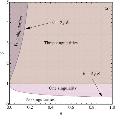
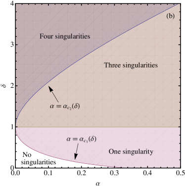
Figure 1: (Color online) The regions in the (a) $\theta,\delta$ and (b) $\alpha,\delta$ spaces, where $g(\lambda)$ has the number of singularities mentioned in the figure. The equations of the boundary lines separating different regions are given in Appendix B. $\alpha_{c_{1}}=1/3$ for $\delta=0$ and $\theta_{c_{2}}\rightarrow 1/3$ as $\delta\rightarrow\infty$. Each of the phase boundaries meet at $\theta=0$ ($\alpha=0$), $\delta=1$.

Now, if $g(\lambda)$ is analytic for $\lambda\in(0,\lambda^{*})$, one can deform the contour along the path of the steepest descent through the saddle-point, and obtain $P(W_{\tau})$ using the usual saddle-point approximation method. However, if $g(\lambda)$ has any singularities, then the straightforward saddle-point method cannot be used, and one would require more sophisticated methods to obtain the asymptotic form of $P(W_{\tau})$. Therefore, it is essential to analyze $g(\lambda)$ for possible singularities. In Appendix B, we examine the terms under the four square roots in the denominator of $g(\lambda)$ in Eq. (16).

In Fig. 1, we show the regions in the $(\theta,\delta)$ and $(\alpha,\delta)$ planes, where $g(\lambda)$ possesses singularities.

IV.1 The case of no singularities

In the singularity free region $\delta<1$, $\theta<\theta_{c_{1}}$ ($\alpha<\alpha_{c_{1}}$), the asymptotic PDF of the work done is obtained by following the usual saddle-point approximation method. We get

$$P(W_{\tau}=w\tau)\approx\frac{g(\lambda^{*})e^{\tau h_{\text{s}}(w)}}{\sqrt{2\pi\tau f^{\prime\prime}_{w}(\lambda^{*})}},$$ (27)

where $h_{\text{s}}(w)$ and $f^{\prime\prime}_{w}(\lambda^{*})$ are given by Eqs. (25) and (26), respectively, and $g(\lambda^{*})$ can be obtained from Eq. (16) while using $\lambda^{*}$ from Eq. (21). Figure 2 shows very good agreement between the form given by Eq. (27) and numerical simulation results for $\theta<\theta_{c_{1}}$.

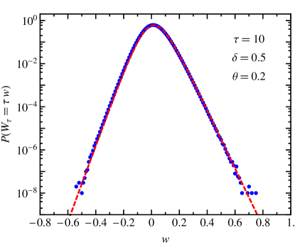
Figure 2: (Color online). $P(W_{\tau})$ against the scaled variable $w=W_{\tau}/\tau$ for $\tau=10$, $\tau_{c}=1$. The points (blue) are obtained from numerical simulation, and the dashed solid lines (red) plot the analytical asymptotic forms given by Eq. (27). $\theta_{c_{1}}=9/35=0.257\dotsc$ for $\delta=1/2$.

IV.2 The case of one singularity

In the case $\delta<1$, $\theta>\theta_{c_{1}}$ where $g(\lambda)$ has only one singularity, or the case $\delta=1$ where only one singularity of $g(\lambda)$ is relevant, we can write

$$g(\lambda)=\frac{g_{1}(\lambda)}{\sqrt{\lambda_{\text{a}}-\lambda}},$$ (28)

where $g_{1}(\lambda)$ is the analytical factor of $g(\lambda)$.

It is evident that for a given value of $\delta$ and $\theta$, the position of the branch point $\lambda_{\text{a}}$ is fixed somewhere between the origin and $\lambda_{+}$. On the other hand, according to Eq. (21), even for a fixed $\theta$, the saddle-point $\lambda^{*}(w)$ moves unidirectionally along the real-$\lambda$ line from $\lambda_{-}$ to $\lambda_{+}$ as one decreases $w$ from $+\infty$ to $-\infty$ in a monotonic manner. Therefore, for sufficiently large $w$, the saddle-point lies in the interval $(\lambda_{-},\lambda_{\text{a}})$, and therefore, the contour of integration in Eq. (19) can be deformed into the steepest descent path (that passes through $\lambda^{*}$) without touching $\lambda_{\text{a}}$ (see Fig. 9). However, as one decreases $w$, the saddle-point hits the branch-point, $\lambda^{*}(w^{*}_{\text{a}})=\lambda_{\text{a}}$, at some specific value $w=w^{*}_{\text{a}}$ given by Eq. (113). For $w<w^{*}_{\text{a}}$, since $\lambda^{*}>\lambda_{\text{a}}$, the steepest descent contour wraps around the branch-cut between $\lambda_{\text{a}}$ and $\lambda^{*}$ as shown in Fig. 10. Leaving the details of the calculation to Appendix C, here we present the main results.

IV.2.1 $w>w^{*}_{\mathrm{a}}$

For $w>w^{*}_{\text{a}}$, following Appendix C.1, we get

$$P(W_{\tau}=w\tau)\approx\frac{g(\lambda^{*})e^{\tau h_{\text{s}}(w)}}{\sqrt{2\pi\tau f^{\prime\prime}_{w}(\lambda^{*})}}\,R_{1}\biggl{(}\sqrt{\tau\bigl{[}h_{\text{a}}(w)-h_{\text{s}}(w)\bigr{]}}\biggr{)},$$ (29)

where the function $R_{1}(z)$ is given by

$$R_{1}(z)=\frac{z}{\sqrt{\pi}}\,e^{z^{2}/2}\,K_{1/4}(z^{2}/2),$$ (30)

with $K_{1/4}(z)$ being the modified Bessel function of the second kind. It follows from the asymptotic form of $K_{1/4}(z)$ that $R_{1}(z\rightarrow\infty)\rightarrow 1$. Therefore, for $w\gg w^{*}_{\text{a}}$, Eq. (29) approaches the form of the usual saddle-point approximation given by Eq. (27). On the other hand, using $K_{1/4}(z)\simeq(1/2)\Gamma(1/4)(z/2)^{-1/4}$ for small $z$, we get $R_{1}(z)\simeq\Gamma(1/4)\sqrt{z/2\pi}$. As $w\rightarrow w^{*}_{\text{a}}$ from above, i.e., when the saddle point approaches the branch point from below, $h_{\text{a}}(w)-h_{\text{s}}(w)\equiv f_{w}(\lambda_{\text{a}})-f_{w}(\lambda^{*})\simeq(\lambda_{\text{a}}-\lambda^{*})^{2}f^{\prime\prime}(\lambda^{*})/2$. Therefore, the expression given by Eq. (29) remains finite, even when the saddle point approaches the singularity, i.e.,

$$P(W_{\tau}=w\tau)\approx\frac{\Gamma(1/4)}{2\pi}\frac{g_{1}(\lambda^{*})e^{\tau h_{\text{s}}(w)}}{[2\tau f^{\prime\prime}_{w}(\lambda^{*})]^{1/4}}\,\quad\text{as}~{}w\rightarrow w^{*}_{\text{a}}.$$ (31)

IV.2.2 $w<w^{*}_{\mathrm{a}}$

For $w<w^{*}_{\text{a}}$, following Appendix C.2, we write

$$P(W_{\tau}=w\tau)\approx P_{\text{B}}(w,\tau)+P_{\text{S}}(w,\tau),$$ (32)

where $P_{\text{B}}(w,\tau)$ is the contribution coming from the integrations along the branch cut and $P_{\text{S}}(w,\tau)$ is the saddle point contribution. Following Appendix C.2.1 we get,

$$P_{\text{B}}(w,\tau)\approx\frac{\widetilde{g}(\lambda_{\text{a}})\,e^{\tau h_{\text{a}}(w)}}{\sqrt{\pi\tau|f^{\prime}_{w}(\lambda_{\text{a}})|}}R_{3}\left(\sqrt{\tau\bigl{[}h_{\text{a}}(w)-h_{\text{s}}(w)\bigr{]}}\right),$$ (33)

where

$$R_{3}(z)=\sqrt{\frac{2z}{\pi}}\,R_{2}(z),$$ (34)

with $R_{2}(z)$ being given by Eq. (137). Using the asymptotic forms of $R_{2}(z)$ given in Appendix C.2.1, we get $R_{3}(z)\rightarrow 1$ in the limit $z\rightarrow\infty$. Therefore,

$$P_{\text{B}}(w,\tau)\sim\frac{\widetilde{g}(\lambda_{\text{a}})e^{\tau h_{\text{a}}(w)}}{\sqrt{\pi\tau|f^{\prime}_{w}(\lambda_{\text{a}})|}}\,\quad\text{for}~{}~{}w\ll w^{*}_{\text{a}}.$$ (35)

As $w\rightarrow w^{*}_{\text{a}}$ (from below), $P_{\text{B}}(w,\tau)\rightarrow 0$.

The contribution coming from the saddle point is given by (see Appendix C.2.2),

$$P_{\text{S}}(w,\tau)\approx\frac{|g(\lambda^{*})|e^{\tau h_{\text{s}}(w)}}{\sqrt{2\pi\tau f^{\prime\prime}_{w}(\lambda^{*})}}\,R_{4}\biggl{(}\sqrt{\tau\bigl{[}h_{\text{a}}(w)-h_{\text{s}}(w)\bigr{]}}\biggr{)},$$ (36)

where the function $R_{4}(z)$ is given by

$$R_{4}(z)= \sqrt{\frac{\pi}{2}}\,z\,e^{z^{2}/2}\bigl{[}I_{-1/4}(z^{2}/2)+I_{1/4}(z^{2}/2)\bigr{]}$$

$$-\frac{4z}{\sqrt{\pi}}\,{}_{2}F_{2}\left(1/2,1;3/4,5/4;z^{2}\right),$$ (37)

where $I_{\pm 1/4}(z)$ are modified Bessel functions of the first kind and ${}_{2}F_{2}(a_{1},a_{2};b_{1},b_{2};z)$ is the generalized hypergeometric function, defined by Eq. (146). The small and large $z$ behaviors of $R_{4}(z)$ are given in Appendix C.2.2.

For $w\ll w^{*}_{\text{a}}$ we get $P_{\text{S}}(w,\tau)\ll P_{\text{B}}(w,\tau)$. On the other hand $P_{\text{S}}(w,\tau)$ acquires the same limiting form as in Eq. (31), when $w\rightarrow w^{*}_{\text{a}}$ (from below).

IV.2.3 Numerical Simulation

We now compare the asymptotic forms presented in this subsection with numerical simulation. In one case, we choose $\delta=1$ and $\theta=4$, for which we get $\lambda_{\pm}=(1\pm\sqrt{2})/2$, $\lambda^{*}(w)=\bigl{(}1-\sqrt{2}w/\sqrt{1+w^{2}}\bigr{)}/2$, $\lambda_{\text{a}}=1/2$, and $w^{*}_{\text{a}}=0$. In an another case, we choose $\delta=1/2$ and $\theta=13.5$, for which $w^{*}_{\text{a}}=-0.0135\dotsc$. Figure 3 shows very good agreement between the analytical and and simulation results.

Figure 3: (Color online). $P(W_{\tau})$ against the scaled variable $w=W_{\tau}/\tau$ for $\tau=10$, $\tau_{c}=1$. The points (blue) are obtained from numerical simulation, and the dashed solid lines (red) plot the analytical asymptotic forms given by Eq. (29) for $w>w^{*}_{\text{a}}$ and Eqs. (32)–(36) for $w<w^{*}_{\text{a}}$, where $w^{*}_{\text{a}}=0$ for $\delta=1,\theta=4$, and $w^{*}_{\text{a}}=-0.0135\dotsc$ for $\delta=0.5,\theta=13.5$.

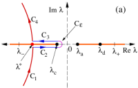
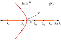
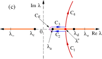
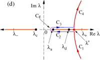
Figure 4: (Color online) Schematic steepest descent contours for the case when there are three branch points at $\lambda_{\text{a}}$, $\lambda_{\text{c}}$ and $\lambda_{\text{d}}$, where $\lambda_{-}<\lambda_{\text{c}}<0<\lambda_{\text{a}}<\lambda_{\text{d}}<\lambda_{+}$; and the saddle point $\lambda^{*}$ lies between (a) $\lambda_{-}$ and $\lambda_{\text{c}}$, (b) $\lambda_{\text{c}}$ and $\lambda_{\text{a}}$, (c) $\lambda_{\text{a}}$ and $\lambda_{\text{d}}$, and (d) $\lambda_{\text{d}}$ and $\lambda_{+}$ respectively.

IV.3 The case of three singularities

Now we consider the case, $\delta>1$ and $\theta>\theta_{c_{2}}$, in which case $g(\lambda)$ has three singularities (see Fig. 1) at $\lambda_{\text{a}}$, $\lambda_{\text{c}}$ and $\lambda_{\text{d}}$ given by Eqs. (103), (105) and (106) respectively; where $\lambda_{-}<\lambda_{\text{c}}<0<\lambda_{\text{a}}<\lambda_{\text{d}}<\lambda_{+}$. Therefore, $g(\lambda)$ can be written as

$$g(\lambda)=\frac{g_{3}(\lambda)}{\sqrt{\lambda-\lambda_{\text{c}}}\sqrt{\lambda_{\text{a}}-\lambda}\sqrt{\lambda_{\text{d}}-\lambda}},$$ (38)

where $g_{3}(\lambda)$ is the analytical factor of $g(\lambda)$. We notice from Eq. (21) that $\lambda^{*}\rightarrow\lambda_{-}$ as $w\rightarrow+\infty$ and $\lambda^{*}$ increases monotonically towards $\lambda_{+}$ with decreasing $w$. Therefore, there are specific values $+\infty>w^{*}_{\text{c}}>w^{*}_{\text{a}}>w^{*}_{\text{d}}>-\infty$ of $w$ given by Eq. (113) at which the saddle point hits the corresponding branch point, i.e., $\lambda^{*}(w^{*}_{\text{c}})=\lambda_{\text{c}}$, $\lambda^{*}(w^{*}_{\text{a}})=\lambda_{\text{a}}$ and $\lambda^{*}(w^{*}_{\text{d}})=\lambda_{\text{d}}$.

IV.3.1 $w>w^{*}_{\text{c}}$

For $w>w^{*}_{\text{c}}$, the saddle point lies between $\lambda_{-}$ and $\lambda_{\text{c}}$. Therefore, as in the case of one singularity discussed above in Sec. IV.2, the contributions comes from the branch point as well as from the saddle point, as shown in Fig. 4 (a). Following the procedure similar to that in the one singularity case (see Appendix C.2), we get

$$P(W_{\tau}=w\tau)\approx \frac{\widetilde{g}(\lambda_{\text{c}})\,e^{\tau h_{\text{c}}(w)}}{\sqrt{\pi\tau|f^{\prime}_{w}(\lambda_{\text{c}})|}}R_{3}\left(\sqrt{\tau\bigl{[}h_{\text{c}}(w)-h_{\text{s}}(w)\bigr{]}}\right)$$

$$+ \frac{|g(\lambda^{*})|e^{\tau h_{\text{s}}(w)}}{\sqrt{2\pi\tau f^{\prime\prime}_{w}(\lambda^{*})}}\,R_{5}\biggl{(}\sqrt{\tau\bigl{[}h_{\text{c}}(w)-h_{\text{s}}(w)\bigr{]}},\sqrt{\tau\bigl{[}h_{\text{a}}(w)-h_{\text{s}}(w)\bigr{]}},\sqrt{\tau\bigl{[}h_{\text{d}}(w)-h_{\text{s}}(w)\bigr{]}}\biggr{)},$$ (39)

where $R_{3}(z)$ is given by Eq. (34), and

$$R_{5}(z_{1},z_{2},z_{3})=\sqrt{\frac{z_{1}z_{2}z_{3}}{\pi}}\int_{0}^{\infty}du\,e^{-u^{2}}\biggl{[}\frac{1}{\sqrt{z_{1}+iu}\sqrt{z_{2}+iu}\sqrt{z_{3}+iu}}-\frac{1}{\sqrt{z_{1}-iu}\sqrt{z_{2}-iu}\sqrt{z_{3}-iu}}\biggr{]}i.$$ (40)

IV.3.2 $w^{*}_{\text{a}}<w<w^{*}_{\text{c}}$

For $w^{*}_{\text{a}}<w<w^{*}_{\text{c}}$, the saddle point lies between $\lambda_{\text{c}}$ and $\lambda_{\text{a}}$. Therefore, the contour of integration can be deformed through the saddle point without crossing any singularity, as shown in Fig. 4 (b). Now, to compute the saddle point contribution one can follow the methods of Appendix C.1, while taking into account of both the singularities $\lambda_{\text{a}}$ and $\lambda_{\text{c}}$. The calculation yields

$$P(W_{\tau}=w\tau)\approx\frac{g(\lambda^{*})e^{\tau h_{\text{s}}(w)}}{\sqrt{2\pi\tau f^{\prime\prime}_{w}(\lambda^{*})}}R_{6}\biggl{(}\sqrt{\tau\bigl{[}h_{\text{c}}(w)-h_{\text{s}}(w)\bigr{]}},\sqrt{\tau\bigl{[}h_{\text{a}}(w)-h_{\text{s}}(w)\bigr{]}},\sqrt{\tau\bigl{[}h_{\text{d}}(w)-h_{\text{s}}(w)\bigr{]}}\biggr{)},$$ (41)

where

$$R_{6}(z_{1},z_{2},z_{3})=\sqrt{\frac{z_{1}z_{2}z_{3}}{\pi}}\int_{-\infty}^{\infty}\frac{e^{-u^{2}}\,du}{\sqrt{z_{1}+iu}\sqrt{z_{2}-iu}\sqrt{z_{3}-iu}}.$$ (42)

As $w\rightarrow w^{*}_{\text{c}}$, the first term of Eq. (39), coming from the integral along the branch cut, goes to zero. On the other hand, it can be shown that $R_{5}(z_{1}\rightarrow 0,z_{2},z_{3})=R_{6}(z_{1}\rightarrow 0,z_{2},z_{3})$. Therefore, Eqs. (39) and (41) approach the same limiting form as $w\rightarrow w^{*}_{\text{c}}$ from the two sides.

IV.3.3 $w^{*}_{\text{d}}<w<w^{*}_{\text{a}}$

For $w^{*}_{\text{d}}<w<w^{*}_{\text{a}}$, the saddle point lies between $\lambda_{\text{a}}$ and $\lambda_{\text{d}}$. Therefore, the deformed contour is as shown in Fig. 4 (c). Combining the contributions from the branch point $\lambda_{\text{a}}$ and the saddle point, we get

$$P(W_{\tau}=w\tau)\approx \frac{\widetilde{g}(\lambda_{\text{a}})\,e^{\tau h_{\text{a}}(w)}}{\sqrt{\pi\tau|f^{\prime}_{w}(\lambda_{\text{a}})|}}R_{7}\biggl{(}\sqrt{\tau\bigl{[}h_{\text{a}}(w)-h_{\text{s}}(w)\bigr{]}},\sqrt{\tau\bigl{[}h_{\text{d}}(w)-h_{\text{s}}(w)\bigr{]}}\biggr{)}$$

$$+ \frac{|g(\lambda^{*})|\,e^{\tau h_{\text{s}}(w)}}{\sqrt{2\pi\tau f^{\prime\prime}_{w}(\lambda^{*})}}R_{8}\biggl{(}\sqrt{\tau\bigl{[}h_{\text{c}}(w)-h_{\text{s}}(w)\bigr{]}},\sqrt{\tau\bigl{[}h_{\text{a}}(w)-h_{\text{s}}(w)\bigr{]}},\sqrt{\tau\bigl{[}h_{\text{d}}(w)-h_{\text{s}}(w)\bigr{]}}\biggr{)},$$ (43)

where

$$R_{7}(z_{1},z_{2})= \sqrt{\frac{2z_{1}(z_{1}+z_{2})}{\pi}}\int_{0}^{z_{1}}\frac{e^{-2z_{1}u+u^{2}}}{\sqrt{u}\sqrt{z_{1}+z_{2}-u}}\,du,$$ (44)

$$\text{and}\quad R_{8}(z_{1},z_{2},z_{3})= \sqrt{\frac{z_{1}z_{2}z_{3}}{\pi}}\int_{0}^{\infty}du\,e^{-u^{2}}\left[\frac{1}{\sqrt{z_{1}+iu}\sqrt{z_{2}+iu}\sqrt{z_{3}-iu}}-\frac{1}{\sqrt{z_{1}-iu}\sqrt{z_{2}-iu}\sqrt{z_{3}+iu}}\right]i.$$ (45)

As $w\rightarrow w^{*}_{\text{a}}$, the first term of Eq. (43), coming from the integral along the branch cut, goes to zero. On the other hand, it can be shown that $R_{6}(z_{1},z_{2}\rightarrow 0,z_{3})=R_{8}(z_{1},z_{2}\rightarrow 0,z_{3})$. Therefore, Eqs. (41) and (43) approach the same limiting form as $w\rightarrow w^{*}_{\text{a}}$ from the two sides.

IV.3.4 $w<w^{*}_{\text{d}}$

Finally, for $w<w^{*}_{\text{d}}$, the saddle point lies between $\lambda_{\text{d}}$ and $\lambda_{+}$. In this case, the integral along the branch cut can be divided into two parts: one, from $\lambda_{\text{a}}$ to $\lambda_{\text{d}}$ and another from $\lambda_{\text{d}}$ to $\lambda^{*}$. Between $\lambda_{\text{d}}$ and $\lambda^{*}$, the the integral above the branch cut exactly cancels the integral below the branch cut. Therefore, the net contribution is the sum of the contributions coming from the integral around the branch cut between $\lambda_{\text{a}}$ and $\lambda_{\text{d}}$, and the contribution of the integral along the contour ($C_{1}$ and $C_{4}$) through the saddle point, for which the calculation is similar to the one given in Appendix C.1. Therefore, we get

$$P(W_{\tau}=w\tau)\approx \frac{\widetilde{g}(\lambda_{\text{a}})\,e^{\tau h_{\text{a}}(w)}}{\sqrt{\pi\tau|f^{\prime}_{w}(\lambda_{\text{a}})|}}R_{9}\biggl{(}\sqrt{\tau\bigl{[}h_{\text{a}}(w)-h_{\text{s}}(w)\bigr{]}},\sqrt{\tau\bigl{[}h_{\text{d}}(w)-h_{\text{s}}(w)\bigr{]}}\biggr{)}$$

$$- \frac{|g(\lambda^{*})|\,e^{\tau h_{\text{s}}(w)}}{\sqrt{2\pi\tau f^{\prime\prime}_{w}(\lambda^{*})}}R_{10}\biggl{(}\sqrt{\tau\bigl{[}h_{\text{c}}(w)-h_{\text{s}}(w)\bigr{]}},\sqrt{\tau\bigl{[}h_{\text{a}}(w)-h_{\text{s}}(w)\bigr{]}},\sqrt{\tau\bigl{[}h_{\text{d}}(w)-h_{\text{s}}(w)\bigr{]}}\biggr{)},$$ (46)

where

$$R_{9}(z_{1},z_{2})=\sqrt{\frac{2z_{1}(z_{1}-z_{2})}{\pi}}\int_{0}^{z_{1}-z_{2}}\frac{e^{-2z_{1}u+u^{2}}\,du}{\sqrt{u}\sqrt{z_{1}-z_{2}-u}},$$ (47)

$$R_{10}(z_{1},z_{2},z_{3})=\sqrt{\frac{z_{1}z_{2}z_{3}}{\pi}}\int_{-\infty}^{\infty}\frac{e^{-u^{2}}\,du}{\sqrt{z_{1}+iu}\sqrt{z_{2}+iu}\sqrt{z_{3}+iu}}.$$ (48)

It is evident from the above equations that $R_{7}(z_{1},0)=R_{9}(z_{1},0)$. Moreover, it can be shown that $R_{10}(z_{1},z_{2},z_{3}\rightarrow 0)=-R_{8}(z_{1},z_{2},z_{3}\rightarrow 0)$. Therefore, Eqs. (43) and (46) approach the same limiting form as $w\rightarrow w^{*}_{\text{d}}$ from the two sides.

IV.4 The case of four singularities

Finally, we consider the case $\delta>1$ and $\theta<\theta_{c_{2}}$, in which case $g(\lambda)$ has four singularities (see Fig. 1) at $\lambda_{\text{a}}$, $\lambda_{\text{b}}$, $\lambda_{\text{c}}$ and $\lambda_{\text{d}}$ given by Eqs. (103)–(106) respectively; where $\lambda_{-}<\lambda_{\text{b}}<\lambda_{\text{c}}<0<\lambda_{\text{a}}<\lambda_{\text{d}}<\lambda_{+}$. Therefore, and $g(\lambda)$ can be written as

$$g(\lambda)=\frac{g_{4}(\lambda)}{\sqrt{\lambda-\lambda_{\text{b}}}\sqrt{\lambda-\lambda_{\text{c}}}\sqrt{\lambda_{\text{a}}-\lambda}\sqrt{\lambda_{\text{d}}-\lambda}},$$ (49)

where $g_{4}(\lambda)$ is the analytical factor of $g(\lambda)$.

Now as $w$ varies from $+\infty$ to $-\infty$, the saddle point hits the branch points, $\lambda^{*}(w^{*}_{i})=\lambda_{i}$ with $i\in\{\text{b, c, a, d}\}$, at specific values of $w$ given by Eq. (113) and $+\infty>w^{*}_{\text{b}}>w^{*}_{\text{c}}>w^{*}_{\text{a}}>w^{*}_{\text{d}}>-\infty$. It is straightforward to generalize the above results to this case of four singularities. Therefore, we only give the results below, without repeating the details.

IV.4.1 $w>w^{*}_{\text{b}}$

For $w>w^{*}_{\text{b}}$, the saddle point lies between $\lambda_{-}$ and $\lambda_{\text{b}}$, and

$$P(W_{\tau}=w\tau)\approx \frac{\widetilde{g}(\lambda_{\text{c}})\,e^{\tau h_{\text{c}}(w)}}{\sqrt{\pi\tau|f^{\prime}_{w}(\lambda_{\text{c}})|}}R_{9}\biggl{(}\sqrt{\tau\bigl{[}h_{\text{c}}(w)-h_{\text{s}}(w)\bigr{]}},\sqrt{\tau\bigl{[}h_{\text{b}}(w)-h_{\text{s}}(w)\bigr{]}}\biggr{)}$$

$$- \frac{|g(\lambda^{*})|\,e^{\tau h_{\text{s}}(w)}}{\sqrt{2\pi\tau f^{\prime\prime}_{w}(\lambda^{*})}}R_{11}\biggl{(}\sqrt{\tau\bigl{[}h_{\text{b}}(w)-h_{\text{s}}(w)\bigr{]}},\sqrt{\tau\bigl{[}h_{\text{c}}(w)-h_{\text{s}}(w)\bigr{]}},\sqrt{\tau\bigl{[}h_{\text{a}}(w)-h_{\text{s}}(w)\bigr{]}},\sqrt{\tau\bigl{[}h_{\text{d}}(w)-h_{\text{s}}(w)\bigr{]}}\biggr{)},$$ (50)

where $R_{9}(z_{1},z_{2})$ is given by Eq. (47) and

$$R_{11}(z_{1},z_{2},z_{3},z_{4})=\sqrt{\frac{z_{1}z_{2}z_{3}z_{4}}{\pi}}\int_{-\infty}^{\infty}\frac{e^{-u^{2}}\,du}{\sqrt{z_{1}-iu}\sqrt{z_{2}-iu}\sqrt{z_{3}-iu}\sqrt{z_{4}-iu}}=\sqrt{\frac{z_{1}z_{2}z_{3}z_{4}}{\pi}}\int_{-\infty}^{\infty}\frac{e^{-u^{2}}\,du}{\sqrt{z_{1}+iu}\sqrt{z_{2}+iu}\sqrt{z_{3}+iu}\sqrt{z_{4}+iu}}.$$ (51)

IV.4.2 $w^{*}_{\text{c}}<w<w^{*}_{\text{b}}$

For $w^{*}_{\text{c}}<w<w^{*}_{\text{b}}$, the saddle point lies between $\lambda_{\text{b}}$ and $\lambda_{\text{c}}$, and

$$P(W_{\tau}=w\tau)\approx \frac{\widetilde{g}(\lambda_{\text{c}})\,e^{\tau h_{\text{c}}(w)}}{\sqrt{\pi\tau|f^{\prime}_{w}(\lambda_{\text{c}})|}}R_{7}\biggl{(}\sqrt{\tau\bigl{[}h_{\text{c}}(w)-h_{\text{s}}(w)\bigr{]}},\sqrt{\tau\bigl{[}h_{\text{b}}(w)-h_{\text{s}}(w)\bigr{]}}\biggr{)}$$

$$+ \frac{|g(\lambda^{*})|\,e^{\tau h_{\text{s}}(w)}}{\sqrt{2\pi\tau f^{\prime\prime}_{w}(\lambda^{*})}}R_{12}\biggl{(}\sqrt{\tau\bigl{[}h_{\text{b}}(w)-h_{\text{s}}(w)\bigr{]}},\sqrt{\tau\bigl{[}h_{\text{c}}(w)-h_{\text{s}}(w)\bigr{]}},\sqrt{\tau\bigl{[}h_{\text{a}}(w)-h_{\text{s}}(w)\bigr{]}},\sqrt{\tau\bigl{[}h_{\text{d}}(w)-h_{\text{s}}(w)\bigr{]}}\biggr{)},$$ (52)

where $R_{7}(z_{1},z_{2})$ is given by Eq. (44) and

$$R_{12}(z_{1},z_{2},z_{3},z_{4})=\sqrt{\frac{z_{1}z_{2}z_{3}z_{4}}{\pi}}\int_{0}^{\infty}du\,e^{-u^{2}}\left[\frac{1}{\sqrt{z_{1}-iu}\sqrt{z_{2}+iu}\sqrt{z_{3}+iu}\sqrt{z_{4}+iu}}-\frac{1}{\sqrt{z_{1}+iu}\sqrt{z_{2}-iu}\sqrt{z_{3}-iu}\sqrt{z_{4}-iu}}\right]i.$$ (53)

IV.4.3 $w^{*}_{\text{a}}<w<w^{*}_{\text{c}}$

For $w^{*}_{\text{a}}<w<w^{*}_{\text{c}}$, the saddle point lies between $\lambda_{\text{c}}$ and $\lambda_{\text{a}}$, and the PDF is given by

$$P(W_{\tau}=w\tau)\approx\frac{g(\lambda^{*})\,e^{\tau h_{\text{s}}(w)}}{\sqrt{2\pi\tau f^{\prime\prime}_{w}(\lambda^{*})}}R_{13}\biggl{(}\sqrt{\tau\bigl{[}h_{\text{b}}(w)-h_{\text{s}}(w)\bigr{]}},\sqrt{\tau\bigl{[}h_{\text{c}}(w)-h_{\text{s}}(w)\bigr{]}},\sqrt{\tau\bigl{[}h_{\text{a}}(w)-h_{\text{s}}(w)\bigr{]}},\sqrt{\tau\bigl{[}h_{\text{d}}(w)-h_{\text{s}}(w)\bigr{]}}\biggr{)},$$ (54)

where

$$R_{13}(z_{1},z_{2},z_{3},z_{4})=\sqrt{\frac{z_{1}z_{2}z_{3}z_{4}}{\pi}}\int_{-\infty}^{\infty}\frac{e^{-u^{2}}\,du}{\sqrt{z_{1}+iu}\sqrt{z_{2}+iu}\sqrt{z_{3}-iu}\sqrt{z_{4}-iu}}.$$ (55)

IV.4.4 $w^{*}_{\text{d}}<w<w^{*}_{\text{a}}$

For $w^{*}_{\text{d}}<w<w^{*}_{\text{a}}$, the saddle point lies between $\lambda_{\text{a}}$ and $\lambda_{\text{d}}$, and

$$P(W_{\tau}=w\tau)\approx \frac{\widetilde{g}(\lambda_{\text{a}})\,e^{\tau h_{\text{a}}(w)}}{\sqrt{\pi\tau|f^{\prime}_{w}(\lambda_{\text{a}})|}}R_{7}\biggl{(}\sqrt{\tau\bigl{[}h_{\text{a}}(w)-h_{\text{s}}(w)\bigr{]}},\sqrt{\tau\bigl{[}h_{\text{d}}(w)-h_{\text{s}}(w)\bigr{]}}\biggr{)}$$

$$+ \frac{|g(\lambda^{*})|\,e^{\tau h_{\text{s}}(w)}}{\sqrt{2\pi\tau f^{\prime\prime}_{w}(\lambda^{*})}}R_{14}\biggl{(}\sqrt{\tau\bigl{[}h_{\text{b}}(w)-h_{\text{s}}(w)\bigr{]}},\sqrt{\tau\bigl{[}h_{\text{c}}(w)-h_{\text{s}}(w)\bigr{]}},\sqrt{\tau\bigl{[}h_{\text{a}}(w)-h_{\text{s}}(w)\bigr{]}},\sqrt{\tau\bigl{[}h_{\text{d}}(w)-h_{\text{s}}(w)\bigr{]}}\biggr{)},$$ (56)

where $R_{7}(z_{1},z_{2})$ is given by Eq. (44) and

$$R_{14}(z_{1},z_{2},z_{3},z_{4})=\sqrt{\frac{z_{1}z_{2}z_{3}z_{4}}{\pi}}\int_{0}^{\infty}du\,e^{-u^{2}}\left[\frac{1}{\sqrt{z_{1}+iu}\sqrt{z_{2}+iu}\sqrt{z_{3}+iu}\sqrt{z_{4}-iu}}-\frac{1}{\sqrt{z_{1}-iu}\sqrt{z_{2}-iu}\sqrt{z_{3}-iu}\sqrt{z_{4}+iu}}\right]i.$$ (57)

IV.4.5 $w<w^{*}_{\text{d}}$

Finally, for $w<w^{*}_{\text{d}}$, the saddle point lies between $\lambda_{\text{d}}$ and $\lambda_{+}$, and

$$P(W_{\tau}=w\tau)\approx \frac{\widetilde{g}(\lambda_{\text{a}})\,e^{\tau h_{\text{a}}(w)}}{\sqrt{\pi\tau|f^{\prime}_{w}(\lambda_{\text{a}})|}}R_{9}\biggl{(}\sqrt{\tau\bigl{[}h_{\text{a}}(w)-h_{\text{s}}(w)\bigr{]}},\sqrt{\tau\bigl{[}h_{\text{d}}(w)-h_{\text{s}}(w)\bigr{]}}\biggr{)}$$

$$- \frac{|g(\lambda^{*})|\,e^{\tau h_{\text{s}}(w)}}{\sqrt{2\pi\tau f^{\prime\prime}_{w}(\lambda^{*})}}R_{11}\biggl{(}\sqrt{\tau\bigl{[}h_{\text{b}}(w)-h_{\text{s}}(w)\bigr{]}},\sqrt{\tau\bigl{[}h_{\text{c}}(w)-h_{\text{s}}(w)\bigr{]}},\sqrt{\tau\bigl{[}h_{\text{a}}(w)-h_{\text{s}}(w)\bigr{]}},\sqrt{\tau\bigl{[}h_{\text{d}}(w)-h_{\text{s}}(w)\bigr{]}}\biggr{)}.$$ (58)

where $R_{9}(z_{1},z_{2})$ and $R_{11}(z_{1},z_{2},z_{3},z_{4})$ are given by Eqs. (47) and (51), respectively.

It can be shown that, when $w\rightarrow w_{i}^{*}$ with $i\in\{\text{a},\text{b},\text{c},\text{d}\}$ from the two sides of $w^{*}_{i}$, the respective expressions of the PDFs, i.e, Eqs. (50) and (52), Eqs. (52) and (54), Eqs. (54) and (56), and Eqs. (56) and (58), respectively, approach the same limiting form.

IV.4.6 Numerical simulation

We now compare the analytical results obtained in this section with numerical simulation. We consider $\delta=5$, for which we have $\theta_{c_{2}}=0.18$. Therefore, $g(\lambda)$ has three singularities for $\theta>\theta_{c_{2}}$, whereas for $\theta<\theta_{c_{2}}$ it has four singularities.

For $\theta=0.5$ the three singularities are located at $\lambda_{\text{c}}=-0.3062\dots$, $\lambda_{\text{a}}=0.3958\dots$ and $\lambda_{\text{d}}=1.3062\dots$, whereas $\lambda_{-}=-0.4848\dots$ and $\lambda_{+}=1.4848\dots$. Figure 5 compares numerical simulation for this case with analytical results obtained above for the case of the three singularities.

On the other hand, for $\theta=0.1$, the four singularities of $g(\lambda)$ are located at at $\lambda_{\text{b}}=-10/7$, $\lambda_{\text{c}}=-1$, $\lambda_{\text{a}}=13/11$, and $\lambda_{\text{d}}=2$. Moreover, $\lambda_{-}=-1.4621\dotsc$ and $\lambda_{+}=2.4621\dotsc$. Figure 6 compares numerical simulation for this case with analytical results obtained above for the case of the four singularities.

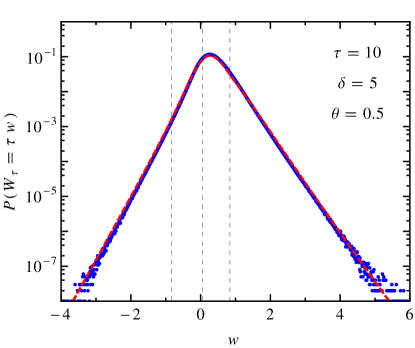
Figure 5: (Color online). $P(W_{\tau})$ against the scaled variable $w=W_{\tau}/\tau$ for $\tau=10$, $\tau_{c}=1$, $\delta=5$, and $\theta=0.5$. The points (blue) are obtained from numerical simulation, and the dashed solid line (red) plots the analytical asymptotic forms given in the text. The vertical dashed lines mark the positions $w^{*}_{\text{c}}=0.8398\dots$, $w^{*}_{\text{a}}=0.06269\dots$ and $w^{*}_{\text{d}}=-0.8398\dots$.

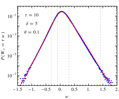
Figure 6: (Color online). $P(W_{\tau})$ against the scaled variable $w=W_{\tau}/\tau$ for $\tau=10$, $\tau_{c}=1$, $\delta=5$ and $\theta=0.1$. The points (blue) are obtained from numerical simulation, and the dashed solid line (red) plots the analytical asymptotic forms given in the text. The vertical dashed lines mark the positions $w^{*}_{\text{b}}=1.4062\dots$, $w^{*}_{\text{c}}=0.3125$, $w^{*}_{\text{a}}=-0.0976\dots$ and $w^{*}_{\text{d}}=-0.3125$.

V Large Deviation Function and Fluctuation Theorem

The large deviation function is defined by

$$h(w)=\lim_{\tau\rightarrow\infty}\frac{1}{\tau}\ln P(W_{\tau}=w\tau).$$ (59)

In other words, the large deviation form of the PDF refers to the ultimate asymptotic form $P(W_{\tau}=w\tau)\sim e^{\tau h(w)}$ while ignoring the subleading corrections. Apart from being an interesting quantity on its own, the large deviation functions have found importance recently in the context of the fluctuation theorem. The latter refers to the relation

$$\lim_{\tau\rightarrow\infty}\frac{1}{\tau}\ln\left[\frac{P(W_{\tau}=+w\tau)}{P(W_{\tau}=-w\tau)}\right]=w.$$ (60)

When the above relation is valid, the large deviation function evidently satisfies the symmetry relation

$$h(w)-h(-w)=w.$$ (61)

Now, as we have seen in the above sections, when $g(\lambda)$ is analytic between the origin and the saddle point, the dominant contribution to $P(W_{\tau})$ comes from the saddle point as given by Eq. (27). On the other hand, when there are singularities between the origin and the saddle point, the most dominant contribution to $P(W_{\tau})$ comes from the singularity closest to the origin (farthest from the saddle point) and lies between the origin and the saddle point. This is because, evidently $-\nu(\lambda)$, and hence the function $f_{w}(\lambda)$, is convex on the interval $[\lambda_{-},\lambda_{+}]$ and $f_{w}(\lambda)$ is minimum at the saddle point $\lambda^{*}$ along the real-$\lambda$ line.

Consequently, for the case $\delta<1$ and $\theta<\theta_{c_{1}}$, where $g(\lambda)$ is analytic on the interval $(\lambda_{-},\lambda_{+})$, the large deviation function is $h(w)=h_{s}(w)$, given by Eq. (25). In this case, $h(w)$ satisfies the above symmetry relation (61), and therefore, the fluctuation theorem is valid. On the other hand, for $\delta<1$ and $\theta>\theta_{c_{1}}$, where $g(\lambda)$ has one singularity at $\lambda_{\text{a}}$, (also for $\delta=1$ and all values of $\theta$, where only the singularity at $\lambda_{\text{a}}$ is relevant), one has

$$h(w)=\begin{cases}h_{s}(w)&\text{for}~{}w>w^{*}_{\text{a}},\\ h_{\text{a}}(w)&\text{for}~{}w<w^{*}_{\text{a}}.\end{cases}$$ (62)

Therefore, it is only when $w^{*}_{\text{a}}<0$ (e.g., when $\theta<4$ for the $\delta=1$ case), the symmetry relation Eq. (61) (and hence the fluctuation theorem) is satisfied only in the specific range $w^{*}_{\text{a}}<w<-w^{*}_{\text{a}}$. Otherwise it is not satisfied.

For the case $\delta>1$, although there are either three or four singularities depending on whether $\theta>\theta_{c_{2}}$ or $\theta<\theta_{c_{2}}$, the singularities closest to the origin (one on each side), namely $\lambda_{\text{c}}$ and $\lambda_{\text{a}}$ are common in both cases. Therefore, for both cases, the large deviation function is given by

$$h(w)=\begin{cases}h_{\text{c}}(w)&\text{for}~{}w>w^{*}_{\text{c}},\\ h_{s}(w)&\text{for}~{}w^{*}_{\text{a}}<w<w^{*}_{\text{c}},\\ h_{\text{a}}(w)&\text{for}~{}w<w^{*}_{\text{a}}.\end{cases}$$ (63)

Since $\lambda_{\text{c}}<0$, it is evident from Eq. (113) that $w^{*}_{\text{c}}>0$. Therefore again, it is only when $w^{*}_{\text{a}}<0$ (e.g., when $\theta<0.365\dots$ for the $\delta=5$ case), the symmetry relation Eq. (61) (and hence the fluctuation theorem) is satisfied only in the specific range $\max(w^{*}_{\text{a}},-w^{*}_{\text{c}})<w<\min(-w^{*}_{\text{a}},w^{*}_{\text{c}})$.

Therefore, for any $\delta$, there exists a $\theta_{c}$, given by $w^{*}_{\text{a}}=0$ (equivalently $\lambda_{\text{a}}=1/2$) as

$$\theta_{c}(\delta)=\frac{3+2\delta+3\delta^{2}+(1-\delta)\sqrt{9+14\delta+9\delta^{2}}}{2\delta^{2}},$$ (64)

and the fluctuation theorem is not valid for $\theta>\theta_{c}$. The $\theta=\theta_{c}(\delta)$ line corresponds to the $\alpha=\alpha_{c}(\delta)$ line in the $(\alpha,\delta)$ plane where

$$\alpha_{c}(\delta)=\frac{3+2\delta+3\delta^{2}+(1-\delta)\sqrt{9+14\delta+9\delta^{2}}}{2(1+\delta)}.$$ (65)

Figure 7 summarizes the state of validity of the fluctuation theorem in the $\delta,\theta$ and $\alpha,\delta$ parameter spaces.

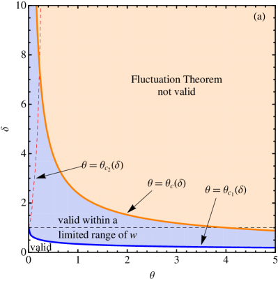
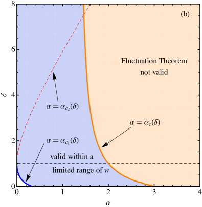
Figure 7: (Color online). The phase diagrams in the parameters space showing the state of the validity of the fluctuation theorem. Apart from the $\theta=\theta_{c}$ and $\alpha=\alpha_{c}$ (orange) lines, the other lines are the same as in Fig. 1. In the (light orange) regions above the (orange) lines $\theta=\theta_{c}$ in (a) and $\alpha=\alpha_{c}$ in (b), the fluctuation theorem is not valid at all, whereas it is always valid in the white regions below the (blue) lines $\theta=\theta_{c_{1}}$ in (a) and $\alpha=\alpha_{c_{1}}$ in (b). In the intermediate (light blue) region, the fluctuation theorem is valid only within a limited range of $w$ given by $w^{*}_{\text{a}}<w<-w^{*}_{\text{a}}$ for $\delta<1$ and $\max(w^{*}_{\text{a}},-w^{*}_{\text{c}})<w<\min(-w^{*}_{\text{a}},w^{*}_{\text{c}})$ for $\delta>1$. For $\delta=0$, we have $\alpha_{c_{1}}=1/3$ and $\alpha_{c}=3$.

VI Summary

Let us now summarize the main contents of the paper. We have obtained analytical results for a system studied recently experimentally Ciliberto:10 . The experimental system consists of a colloidal particle in water and confined in an optical trap which is modulated according to an Ornstein-Uhlenbeck process. This system is described by a set of coupled Langevin equations. We have computed the PDF of the work done by the modulating trap on the Brownian particle in a given time $\tau$, for large $\tau$. The moment generating function of the work has the $\bigl{\langle}e^{-\lambda W_{\tau}}\bigr{\rangle}\approx g(\lambda)\,e^{\tau\mu(\lambda)}$ for large $\tau$. Inverting this, we obtain the PDF of the work within the saddle point approximation.

The results can be described in terms of two independent parameters: (1) the parameter $\theta$ that quantifies the relative strength of the external noise that generates the Ornstein-Uhlenbeck process for the trap modulation, with respect to the thermal fluctuations, and (2) the ratio $\delta=\tau_{0}/\tau_{\gamma}$ of the correlation time of the trap modulation to the viscous relaxation time of the particle in the trap without any modulation. We find that the cumulant generating function $\mu(\lambda)$ is analytic in a (real) interval $(\lambda_{-},\lambda_{+})$ and the saddle point lies within this interval — here $\lambda_{\pm}$ depends on the values of $\theta,\delta$. On the other hand, depending on the values of the pair $(\theta,\delta)$, the function $g(\lambda)$ behaves differently. For $\delta<1$, there exists a value $\theta_{c_{1}}(\delta)$ such that $g(\lambda)$ is analytic in the interval $(\lambda_{-},\lambda_{+})$ for $\theta<\theta_{c_{1}}$ whereas it has a branch point for $\theta>\theta_{c_{1}}$. For $\delta>1$, there again exists a $\theta_{c_{2}}(\delta)$, and $g(\lambda)$ has either three or four branch points depending on whether $\theta>\theta_{c_{2}}$ or $\theta<\theta_{c_{2}}$. For $\delta=1$, there are three branch points of which two coincide with $\lambda_{\pm}$. We have done the analysis in each of these regions and obtained the asymptotic form of the PDF accordingly. We have compared our analytical results with simulation results on this system and found very good agreement between the two.

The calculation also gives the large deviation function as a by-product, using which we check the validity of the so-called fluctuation theorem for this context. We find that in the region $\delta<1,\theta<\theta_{c_{1}}$, it is always valid. Outside this parameter region, there exists a $\theta_{c}(\delta)$ and the fluctuation theorem is valid for a limited range of $w$ around zero when $\theta<\theta_{c}$. For $\theta>\theta_{c}$, the fluctuation theorem is not valid at all (see Fig. 7).

Finally, we would like to point out that it is very easy to generalize the analysis of the paper to the case of a Brownian particle subjected to any exponentially correlated external random force. Moreover, the asymptotic analysis (steepest descent method with branch points.) carried out in this paper should be applicable for finding asymptotic approximations of similar integrals in general.

Appendix A Calculation of the Moment Generating Function

The evolution equations (1) and (2) can be presented in the matrix form

$$\frac{dU}{dt}=-\frac{1}{\tau_{0}}{A}U+\eta(t),$$ (66)

where $U=(x,y)^{T}$ and $\eta=(\xi,\zeta)^{T}$ are column vectors and ${A}$ is a $2\times 2$ matrix given by

$${A}=\begin{pmatrix}\delta&-\delta\\ 0&1\end{pmatrix}.$$ (67)

Using the integral representation of $\delta$-function, the restricted moment generating function defined by Eq. (7)

$$Z(\lambda,U,\tau|U_{0})=\int\frac{d^{2}\sigma}{(2\pi)^{2}}e^{i\sigma^{T}U}\bigl{\langle}e^{-\lambda W_{\tau}-i\sigma^{T}U(\tau)}\bigr{\rangle}_{U_{0}},$$ (68)

where $\sigma^{T}=(\sigma_{1},\sigma_{2})$.

Substituting $dx/dt$ form Eq. (1) in Eq. (3) we get

$$W_{\tau}=\int_{0}^{\tau}dt\,\left[-\frac{\delta^{2}}{\tau_{0}^{2}D}y(x-y)+\frac{\delta}{\tau_{0}D}y\xi\right],$$ (69)

which is useful to rewrite as

$$W_{\tau}=\frac{1}{2}\int_{0}^{\tau}dt\left[\frac{1}{\tau_{0}^{2}}U^{T}{A}_{1}U+\frac{1}{\tau_{0}}\bigl{(}U^{T}{A}_{2}^{T}\eta+\eta^{T}{A}_{2}U\bigr{)}\right],$$ (70)

where

$${A}_{1}=\frac{\delta^{2}}{D}\begin{pmatrix}0&-1\\ -1&2\\ \end{pmatrix}\quad\text{and}\quad{A}_{2}=\frac{\delta}{D}\begin{pmatrix}0&1\\ 0&0\\ \end{pmatrix}.$$ (71)

Now, we proceed by defining the finite-time Fourier transforms and their inverses as follows:

$$[\widetilde{U}(\omega_{n}),\widetilde{\eta}(\omega_{n})] =\frac{1}{\tau}\int_{0}^{\tau}dt[U(t),\eta(t)]\exp(-i\omega_{n}t),$$ (72)

$$[U(t),\eta(t)] =\sum_{n=-\infty}^{\infty}[\widetilde{U}(\omega_{n}),\widetilde{\eta}(\omega_{n})]\exp(i\omega_{n}t),$$ (73)

with $\omega_{n}=2\pi n/\tau$. In the frequency domain, the Gaussian noise configurations denoted by $[{\eta(t):0<t<\tau}]$ is described by the infinite sequence $[\widetilde{\eta}(\omega_{n}):n=-\infty,...,-1,0,+1,...,\infty]$ of Gaussian random variables with the correlation

$$\langle\widetilde{\eta}(\omega)\widetilde{\eta}^{T}(\omega^{\prime})\rangle=\frac{2D}{\tau}\delta(\omega+\omega^{\prime})\,\mathrm{diag}(1,\theta).$$ (74)

In terms of the Fourier transform Eq. (70) can be written as

$$W_{\tau}=\frac{\tau}{2}\sum_{n=-\infty}^{\infty}\biggl{[}\frac{1}{\tau_{0}^{2}}\widetilde{U}^{T}(\omega_{n}){A}_{1}\widetilde{U}(-\omega_{n})\\ +\frac{1}{\tau_{0}}\Bigl{\{}\widetilde{U}^{T}(\omega_{n}){A}_{2}^{T}\widetilde{\eta}(-\omega_{n})+\widetilde{\eta}^{T}(\omega_{n}){A}_{2}\widetilde{U}(-\omega_{n})\Bigr{\}}\biggr{]}.$$ (75)

Equation (66) gives

$$\widetilde{U}(\omega_{n})=\tau_{0}{G}\widetilde{\eta}(\omega_{n})-\frac{\tau_{0}}{\tau}{G}\Delta U,$$ (76)

where ${G}=[iuI+{A}]^{-1}$ with $u=\omega_{n}\tau_{0}$, $\Delta U=U(\tau)-U(0)$, and $I$ being the identity matrix. The elements of $G$ are: $G_{11}=(\delta+iu)^{-1}$, $G_{22}=(1+iu)^{-1}$, $G_{12}=\delta G_{11}G_{22}$, and $G_{21}=0$. Note that ${G}(-u)={G}^{*}(u)$, $\widetilde{\eta}(-\omega)=\widetilde{\eta}^{*}(\omega)$, and $\widetilde{U}(-\omega)=\widetilde{U}^{*}(\omega)$. Substituting $\widetilde{U}$ in Eq. (70), and grouping the negative $n$ indices together with their positive counterparts in the summation, we get

$$W_{\tau}=\Bigl{[} \frac{1}{2}\tau\widetilde{\eta}_{0}^{T}\bigl{(}G_{0}^{T}A_{1}G_{0}+A_{2}G_{0}+G_{0}^{T}A_{2}^{T}\bigr{)}\widetilde{\eta}_{0}$$

$$-\Delta U^{T}\bigl{(}G_{0}^{T}A_{1}G_{0}+G_{0}^{T}A_{2}^{T}\bigr{)}\widetilde{\eta}_{0}$$

$$+\frac{1}{2\tau}\Delta U^{T}\bigl{(}G_{0}^{T}A_{1}G_{0}\bigr{)}\Delta U\Bigr{]}$$

$$+\sum_{n=1}^{\infty}\Bigl{[} \tau\widetilde{\eta}^{T}\bigl{(}G^{T}A_{1}G^{*}+A_{2}G^{*}+G^{T}A_{2}^{T}\bigr{)}\widetilde{\eta}^{*}$$

$$-\widetilde{\eta}^{T}\bigl{(}G^{T}A_{1}G^{*}+A_{2}G^{*}\bigr{)}\Delta U$$

$$-\Delta U^{T}\bigl{(}G^{T}A_{1}G^{*}+G^{T}A_{2}^{T}\bigr{)}\widetilde{\eta}^{*}$$

$$+\frac{1}{\tau}~{}\Delta U^{T}\bigl{(}G^{T}A_{1}G^{*}\bigr{)}\Delta U\Bigr{]},$$ (77)

in which ${G}_{0}={G}(u=0)={A}^{-1}$ and $\widetilde{\eta}_{0}=\widetilde{\eta}(0)$.

Next, we we express $U(\tau)$ in terms of the Fourier series

$$U(\tau)=\lim_{\epsilon\rightarrow 0}\sum_{n=-\infty}^{\infty}\widetilde{U}(\omega_{n})e^{-i\omega_{n}\epsilon}.$$ (78)

While inserting $\widetilde{U}$ from Eq. (76) into the above equation, we observe that $(1/\tau)\sum_{n}Ge^{-i\omega_{n}\epsilon}\rightarrow 0$ as $\tau\rightarrow\infty$. This is because in the large-$\tau$ limit, the summation can be converted to an integral which can be closed via the lower half plane, and the $G$ is analytic there. Thus, using only the first term of Eq. (76), we get

$$\sigma^{T}U(\tau) =\tau_{0}\sigma^{T}G_{0}\widetilde{\eta}_{0}$$

$$+\tau_{0}\sum_{n=1}^{\infty}\bigl{[}e^{-i\omega_{n}\epsilon}\widetilde{\eta}^{T}G^{T}\sigma+e^{i\omega_{n}\epsilon}\sigma^{T}G^{*}\widetilde{\eta}^{*}\bigr{]}.$$ (79)

Using this expression as well as $W_{\tau}$ from above in Eq. (68), we get

$$Z(\lambda,U,\tau|U_{0})=\int\frac{d^{2}\sigma}{(2\pi)^{2}}e^{i\sigma^{T}U}\prod_{n=0}^{\infty}\bigl{\langle}e^{s_{n}}\bigr{\rangle},$$ (80)

where $s_{n}$ is quadratic in $\widetilde{\eta}$, given by

$$s_{0}=-\frac{\lambda\tau}{2}\widetilde{\eta}_{0}^{T}B_{0}\widetilde{\eta}_{0}+\alpha_{0}^{T}\widetilde{\eta}_{0}-\frac{\lambda}{2\tau}\Delta U^{T}G_{0}^{T}A_{1}G_{0}\Delta U,$$ (81)

and

$$s_{n}= -\lambda\tau\widetilde{\eta}^{T}B_{n}\widetilde{\eta}^{*}+\widetilde{\eta}^{T}\alpha_{n}+\alpha_{-n}^{T}\widetilde{\eta}^{*}$$

$$-\frac{\lambda}{\tau}\Delta U^{T}G^{T}A_{1}G^{*}\Delta U\quad\text{for}\quad n\geq 1,$$ (82)

in which we have used the following definitions:

$$B_{n} =G^{T}A_{1}G^{*}+A_{2}G^{*}+G^{T}A_{2}^{T},$$ (83)

$$B_{0} =G_{0}^{T}A_{1}G_{0}+A_{2}G_{0}+G_{0}^{T}A_{2}^{T},$$ (84)

$$\alpha_{n} =\lambda\bigl{[}G^{T}A_{1}G^{*}+A_{2}G^{*}\bigr{]}\Delta U-i\tau_{0}e^{-i\omega_{n}\epsilon}G^{T}\sigma,$$ (85)

$$\alpha_{-n}^{T} =\lambda\Delta U^{T}\bigl{[}G^{T}A_{1}G^{*}+G^{T}A_{2}^{T}\bigr{]}-i\tau_{0}e^{i\omega_{n}\epsilon}\sigma^{T}G^{*}.$$ (86)

Therefore, calculating the average $\langle e^{s_{n}}\rangle$ independently for each $n\geq 1$ with respect to the Gaussian PDF $P(\widetilde{\eta})=\pi^{-2}(\det\Lambda)^{-1}\exp(-\widetilde{\eta}^{T}\Lambda^{-1}\widetilde{\eta}^{*})$ with $\Lambda=(2D/\tau)\mathrm{diag}(1,\theta)$ we get

$$\bigl{\langle}e^{s_{n}}\bigr{\rangle}=\frac{\exp\bigl{(}\alpha_{-n}^{T}\Omega_{n}^{-1}\alpha_{n}-\frac{\lambda}{\tau}\Delta U^{T}G^{T}A_{1}G^{*}\Delta U\bigr{)}}{\det(\Lambda\Omega_{n})},$$ (87)

where $\Omega_{n}=\tau(\lambda B_{n}+\tau^{-1}\Lambda^{-1})$. For the $n=0$ term, calculating the average $\langle e^{s_{0}}\rangle$ with respect to the Gaussian PDF $P(\widetilde{\eta}_{0})=(2\pi)^{-1}(\det\Lambda)^{-1/2}\exp(-\frac{1}{2}\widetilde{\eta}_{0}^{T}\Lambda^{-1}\widetilde{\eta}_{0})$ we get

$$\bigl{\langle}e^{s_{0}}\bigr{\rangle}=\frac{\exp\bigl{(}\frac{1}{2}\alpha_{0}^{T}\Omega_{0}^{-1}\alpha_{0}-\frac{\lambda}{2\tau}\Delta U^{T}G_{0}^{T}A_{1}G_{0}\Delta U\bigr{)}}{\sqrt{\det(\Lambda\Omega_{0})}}.$$ (88)

Since, $\langle e^{s_{n}}\rangle=\langle e^{s_{-n}}\rangle$, the product in Eq. (80) yields

$$\prod_{n=0}^{\infty}\bigl{\langle}e^{s_{n}}\bigr{\rangle}=\exp\biggl{(}-\frac{1}{2}\sum_{n=-\infty}^{\infty}\ln\bigl{[}\det(\Lambda\Omega_{n})\bigr{]}\biggr{)}\\ \times\exp\biggl{(}\frac{1}{2\tau}\sum_{n=-\infty}^{\infty}\bigl{[}\alpha_{-n}^{T}\tau\Omega_{n}^{-1}\alpha_{n}-\lambda\Delta U^{T}G^{T}A_{1}G^{*}\Delta U\bigr{]}\biggr{)}.$$ (89)

The determinant in the above expression is found to be

$$\det(\Lambda\Omega_{n})=[1+4\theta\lambda(1-\lambda)\delta^{2}u^{2}|G_{11}|^{2}|G_{22}|^{2}].$$ (90)

Now, taking the large $\tau$ limit, we replace the summations over $n$ by integrals over $\omega$, i.e., $\sum_{n}\rightarrow\tau\int\frac{d\omega}{2\pi}$. After, evaluating the integral, the argument of the exponential in first line of Eq. (89) yields

$$-\frac{\tau/\tau_{0}}{4\pi}\int_{-\infty}^{\infty}du\,\ln\bigl{[}\det(\Lambda\Omega_{n})\bigr{]}=\tau\mu(\lambda),$$ (91)

where $\mu(\lambda)$ is given by Eq. (11). Similarly, converting the argument of the exponential in the second line of Eq. (89) in the integral forms, after some manipulation we get

$$\prod_{n=0}^{\infty}\bigl{\langle}e^{s_{n}}\bigr{\rangle}\approx e^{\tau\mu(\lambda)}\exp\biggl{[}-\frac{1}{2}\sigma^{T}H_{1}\sigma+i\Delta U^{T}H_{2}\sigma+\frac{1}{2}\Delta U^{T}H_{3}\Delta U\biggr{]},$$ (92)

in which $H_{1}$, $H_{2}$, and $H_{3}$ are given by

$$H_{1} =\frac{D\tau_{0}}{2\pi}\int_{-\infty}^{\infty}du\,G^{*}\widetilde{\Omega}^{-1}G^{T},$$ (93)

$$H_{2} =-\lim_{\epsilon\rightarrow 0}\frac{\lambda}{2\pi}\int_{-\infty}^{\infty}du\,e^{iu\epsilon/\tau_{0}}\,(G^{\dagger}\widetilde{A}_{1}G+G^{\dagger}\widetilde{A}_{2}^{T})(\widetilde{\Omega}^{-1})^{*}G^{\dagger},$$ (94)

$$H_{3} =\frac{\lambda^{2}}{2\pi}\frac{1}{D\tau_{0}}\int_{-\infty}^{\infty}du\,(G^{T}\widetilde{A}_{1}G^{*}+G^{T}\widetilde{A}_{2}^{T})\widetilde{\Omega}^{-1}$$

$$\qquad\times(G^{T}\widetilde{A}_{1}G^{*}+\widetilde{A}_{2}G^{*})-\frac{\lambda}{2\pi}\frac{1}{D\tau_{0}}\int_{-\infty}^{\infty}du~{}[G^{T}\widetilde{A}_{1}G^{*}],$$ (95)

where we have used where $\widetilde{\Omega}_{n}=\tau^{-1}D\Omega_{n}$ and $\widetilde{A}_{1,2}=DA_{1,2}$ so that the integrands remain dimensionless and dimensions are carried outside to the integrals. We then evaluate the integrals performing the method of contours in the complex $u$ plane, and using $G^{*}(u)+G(u)=2GAG^{*}$ and $G^{*}(u)-G(u)=2iuGG^{*}$, which yields

$$H_{1}(\lambda) =\frac{D\tau_{0}}{\delta(1+\delta)\nu(\lambda)}\begin{pmatrix}1+\delta+\theta\delta^{2}&\theta\delta^{2}\\ \theta\delta^{2}&\theta\delta+\theta\delta^{2}\\ \end{pmatrix},$$ (96)

$$H_{2}(\lambda) =-\frac{\nu(\lambda)-1}{2\nu(\lambda)}\begin{pmatrix}1&0\\ 0&1\\ \end{pmatrix}-\frac{\lambda\delta}{(1+\delta)\nu(\lambda)}\begin{pmatrix}\theta\delta&\theta\delta\\ 1&0\\ \end{pmatrix},$$ (97)

$$H_{3}(\lambda) =\frac{\lambda\delta^{2}}{D\tau_{0}(1+\delta)\nu(\lambda)}\begin{pmatrix}\lambda\theta\delta&1\\ 1&\lambda-1\\ \end{pmatrix}.$$ (98)

Finally, inserting Eq. (92) in Eq. (80), and performing the Gaussian integral over $\sigma$ while using the facts that $H_{1}$ and $H_{3}$ are symmetric and $H_{3}=H_{1}^{-1}H_{2}^{T}+H_{2}H_{1}^{-1}H_{2}^{T}$ we get

$$Z(\lambda,U,\tau|U_{0})\approx e^{\tau\mu(\lambda)}\exp\left(-\frac{1}{2}U_{0}^{T}L_{2}(\lambda)U_{0}\right)\\ \times\frac{1}{2\pi\sqrt{\det H_{1}(\lambda)}}\exp\left(-\frac{1}{2}U^{T}L_{1}(\lambda)U\right),$$ (99)

with $L_{1}(\lambda)=H_{1}^{-1}+H_{1}^{-1}H_{2}^{T}$ and $L_{2}(\lambda)=-H_{1}^{-1}H_{2}^{T}$. From the above equation, it is trivial to identify $\chi(U_{0},\lambda)$ and $\Psi(U,\lambda)$ used in Eq. (10). Since, $L_{1}+L_{2}=H_{1}^{-1}$, it is evident that $\int\chi(U,\lambda)\Psi(U,\lambda)\,dU=1$.

Application of the Langevin operator given by Eq. (9) on $\Psi(U,\lambda)$ yields

$$\mathcal{L_{\lambda}}\psi(U,\lambda) =\biggl{[}D\bigl{(}L_{1}^{1,1}\bigr{)}^{2}+\alpha D\bigl{(}L_{1}^{1,2}\bigr{)}^{2}-\frac{\delta}{\tau_{0}}L_{1}^{1,1}\biggr{]}x^{2}\psi(U,\lambda)$$

$$+\biggl{[}D\bigl{(}L_{1}^{1,2}\bigr{)}^{2}+\alpha D\bigl{(}L_{1}^{2,2}\bigr{)}^{2}+\frac{\delta}{\tau_{0}}(1-2\lambda)L_{1}^{1,2}$$

$$\qquad-\frac{1}{\tau_{0}}L_{1}^{2,2}-\frac{\delta^{2}}{D\tau_{0}^{2}}\lambda(1-\lambda)\biggr{]}y^{2}\psi(U,\lambda)$$

$$+\biggl{[}2DL_{1}^{1,1}L_{1}^{1,2}+2D\alpha L_{1}^{1,2}L_{1}^{2,2}+\frac{\delta}{\tau_{0}}(1-2\lambda)L_{1}^{1,1}$$

$$\qquad-\frac{1+\delta}{\tau_{0}}L_{1}^{1,2}+\frac{\delta^{2}}{D\tau_{0}^{2}}\lambda\biggr{]}xy\psi(U,\lambda)$$

$$+\biggl{[}-DL_{1}^{1,1}-\alpha DL_{1}^{2,2}+\frac{1+\delta}{\tau_{0}}\biggr{]}\psi(U,\lambda),$$ (100)

where $L_{1}^{i,j}$ denotes the $(i,j)$-th element of the matrix $L_{1}$. Using the explicit expressions on the right-hand side of the above equation, after simplification, we find the coefficients of $x^{2}\Psi(U,\lambda)$, $y^{2}\Psi(U,\lambda)$, and $xy\Psi(U,\lambda)$ to be zero. The last term in square brackets in front of $\Psi(U,\lambda)$ yields $\mu(\lambda)$ given by Eq. (11). This verifies the eigenvalue equation $\mathcal{L}_{\lambda}\Psi(U,\lambda)=\mu(\lambda)\Psi(U,\lambda)$.

The steady-state of the system is given by

$$P_{\text{SS}}(U)=\Psi(U,0)=\frac{\exp\left(-\frac{1}{2}U^{T}H_{1}^{-1}(0)U\right)}{2\pi\sqrt{\det H_{1}(0)}}.$$ (101)

Integrating Eq. (68) over $U$ and then averaging over the initial condition $U_{0}$ with respect to the steady state distribution $P_{\text{SS}}(U_{0})$, we obtain $Z(\lambda)$ given by Eq. (15), with

$$g(\lambda) =\bigl{(}\det H_{1}(\lambda)\det H_{1}(0)\det L_{1}(\lambda)\det[H_{1}^{-1}(0)+L_{2}(\lambda)]\bigr{)}^{-1/2}$$

$$=\bigl{(}\det[1-\nu(\lambda)H_{2}^{T}(\lambda)]\det[1+H_{2}^{T}(\lambda)]\bigr{)}^{-1/2},$$ (102)

where to obtain the second expression, we have substituted the expressions of $L_{1}$, $L_{2}$ and $H_{1}(0)=\nu(\lambda)H_{1}(\lambda)$. Inserting the matrix $H_{2}$ and evaluating the determinants, after simplification, we obtain Eq. (16).

Appendix B Singularities of $g(\lambda)$

From Eq. (23) we recall that $\nu(\lambda_{\pm})=0$ and $\nu(\lambda)>0$ (is a semicircle) for $\lambda\in(\lambda_{-},\lambda_{+})$. Moreover, all the four functions $1\pm 2b_{\pm}\lambda$ are linear in $\lambda$ with slopes $\pm 2b_{\pm}$ (where all four combinations of the two $\pm$ signs are considered). Therefore, for example, if $(1-2b_{+}\lambda)$ has opposite signs at the two end points $\lambda_{\pm}$, then the function $[\nu(\lambda)+(1-2b_{+}\lambda)]$ must cross zero at some intermediate $\lambda$. This is also true for the other three cases. From Eqs. (17) and (22) respectively, we note that $b_{+}>0$, $b_{-}<0$ and $\lambda_{+}>0$, $\lambda_{-}<0$. One can therefore determine whether $g(\lambda)$ has a singularity as follows (see Fig. 8):

1. Evidently, $1-2b_{+}\lambda_{-}>0$. Thus, $\nu(\lambda_{\text{a}})+1-2b_{+}\lambda_{\text{a}}=0$ for a specific $\lambda_{\text{a}}\in(\lambda_{-},\lambda_{+})$ if and only if $1-2b_{+}\lambda_{+}<0$. When this happens [see Fig. 8 (a)], the position of the singularity can be found as

   $$\lambda_{\text{a}}=(a+b_{+})/(a+b_{+}^{2}).$$ (103)

   It is evident that $\lambda_{\text{a}}>0$.

2. Evidently, $1-2b_{-}\lambda_{+}>0$. Thus, $\nu(\lambda_{\text{b}})+1-2b_{-}\lambda_{\text{b}}=0$ for a specific $\lambda_{\text{b}}\in(\lambda_{-},\lambda_{+})$ if and only if $1-2b_{-}\lambda_{-}<0$. When this happens [see Fig. 8 (b)], the position of the singularity can be found as

   $$\lambda_{\text{b}}=(a+b_{-})/(a+b_{-}^{2})$$ (104)

   and it can be shown that $\lambda_{\text{b}}<0$.

3. Evidently, $1+2b_{+}\lambda_{+}>0$. Thus, $\nu(\lambda_{\text{c}})+1+2b_{+}\lambda_{\text{c}}=0$ for a specific $\lambda_{\text{c}}\in(\lambda_{-},\lambda_{+})$ if and only if $1+2b_{+}\lambda_{-}<0$. When this happens [see Fig. 8 (c)], the position of the singularity can be found as

   $$\lambda_{\text{c}}=(a-b_{+})/(a+b_{+}^{2})$$ (105)

   and it can be shown that $\lambda_{\text{c}}<0$.

4. Evidently, $1+2b_{-}\lambda_{-}>0$. Thus, $\nu(\lambda_{\text{d}})+1+2b_{-}\lambda_{\text{d}}=0$ for a specific $\lambda_{\text{d}}\in(\lambda_{-},\lambda_{+})$ if and only if $1+2b_{-}\lambda_{+}<0$. When this happens [see Fig. 8 (d)], the position of the singularity can be found as

   $$\lambda_{\text{d}}=(a-b_{-})/(a+b_{-}^{2}).$$ (106)

   It is evident that $\lambda_{\text{d}}>0$. Moreover, it can be shown that $\lambda_{\text{c}}+\lambda_{\text{d}}=1$.

It is easily seen that the singularities of $g(\lambda)$ are branch points (square root singularities) and the function $f_{w}(\lambda)$ at these singularities is given by

$$h_{i}(w):=f_{w}(\lambda_{i})=\frac{1}{2}\bigl{[}1-\nu(\lambda_{i})\bigr{]}+\lambda_{i}w,$$ (107)

where the index $i$ stands for one of the indices from the set $\{\text{a, b, c, d}\}$. Substituting $\nu(\lambda_{i})$ at the singularities using the conditions from above, we get

$$h_{\text{a}}(w) =(1-b_{+}\lambda_{\text{a}})+\lambda_{\text{a}}w,$$ (108)

$$h_{\text{b}}(w) =(1-b_{-}\lambda_{\text{b}})+\lambda_{\text{b}}w,$$ (109)

$$h_{\text{c}}(w) =(1+b_{+}\lambda_{\text{c}})+\lambda_{\text{c}}w,$$ (110)

$$h_{\text{d}}(w) =(1+b_{-}\lambda_{\text{d}})+\lambda_{\text{d}}w.$$ (111)

It is also useful to define the non-singular part of $g(\lambda)$ at a singularity as

$$\widetilde{g}(\lambda_{i})=\lim_{\lambda\rightarrow\lambda_{i}}\bigl{|}(\lambda-\lambda_{i})^{1/2}g(\lambda)\bigr{|}.$$ (112)

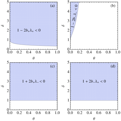
Figure 8: (Color online) In the shaded regions of the $(\theta,\delta)$ plane in the figures (a), (b), (c) and (d), the respective mathematical conditions given there are satisfied and consequently $g(\lambda)$ possesses singularities at $\lambda_{\text{a}}$, $\lambda_{\text{b}}$, $\lambda_{\text{c}}$, and $\lambda_{\text{d}}$ respectively, given by Eqs. (103)–(106).

We note that the for a given set of parameters $\theta$ (or $\alpha$) and $\delta$, the position of the singularities (whenever they exist) are fixed within the interval $(\lambda_{-},\lambda_{+})$. The specific values of $w$ at which the saddle point coincides with one of the singularities is obtained by solving $\lambda^{*}(w^{*}_{i})=\lambda_{i}$ as

$$w^{*}_{i}=\frac{(1-2\lambda_{i})\sqrt{a}}{\sqrt{(1+1/a)-(2\lambda_{i}-1)^{2}}}.$$ (113)

Since, $(1+1/a)=(2\lambda_{\pm}-1)^{2}$ and $\lambda_{-}<\lambda_{i}<\lambda_{+}$, the term under the square root in the above equation is always positive.

B.1 The case: $\delta<1$

For any $\delta<1$, there exists a $\theta_{c_{1}}$ given by the solution of $1-2b_{+}\lambda_{+}=0$ as

$$\theta_{c_{1}}(\delta)=\frac{\left(1-\delta^{2}\right)^{2}}{\delta^{2}\left(3+10\delta+3\delta^{2}\right)},$$ (114)

and for $\theta<\theta_{c_{1}}$ the function $g(\lambda)$ has no singularities whereas it has one singularity for $\theta>\theta_{c_{1}}$. As $\delta\rightarrow 0$ we get $\theta_{c_{1}}\simeq 1/(3\delta^{2})$ whereas $\theta_{c_{1}}\simeq(1-\delta)^{2}/4$ as $\delta\rightarrow 1^{-}$.

The $\theta=\theta_{c_{1}}(\delta)$ line corresponds to the $\alpha=\alpha_{c_{1}}(\delta)$ line in the $(\alpha,\delta)$ plane, where

$$\alpha_{c_{1}}(\delta)=\frac{(1+\delta)\left(1-\delta\right)^{2}}{3+10\delta+3\delta^{2}}.$$ (115)

B.2 The case: $\delta>1$

For $\delta>1$, there again exists a $\theta_{c_{2}}$ given by the solution of $1-2b_{-}\lambda_{-}=0$ as

$$\theta_{c_{2}}(\delta)=\frac{\left(\delta^{2}-1\right)^{2}}{\delta^{2}\left(3+10\delta+3\delta^{2}\right)},$$ (116)

and $g(\lambda)$ has either three or four singularities depending on whether $\theta>\theta_{c_{2}}$ or $\theta<\theta_{c_{2}}$. In the limit $\delta\rightarrow\infty$ we get $\theta_{c_{2}}=1/3$ and $\theta_{c_{2}}\rightarrow 0$ as $\delta\rightarrow 1$. More precisely, $\theta_{c_{2}}\simeq 1/3-10/(9\delta)$ as $\delta\rightarrow\infty$, whereas $\theta_{c_{2}}\simeq(\delta-1)^{2}/4$ as $\delta\rightarrow 1^{+}$.

The $\theta=\theta_{c_{2}}(\delta)$ line corresponds to the $\alpha=\alpha_{c_{2}}(\delta)$ line in the $(\alpha,\delta)$ plane, where

$$\alpha_{c_{2}}(\delta)=\frac{(1+\delta)\left(\delta-1\right)^{2}}{3+10\delta+3\delta^{2}}.$$ (117)

B.3 The case: $\delta=1$

It is instructive to illustrate the particular case of $\delta=1$, for which we have $\alpha=\theta/2$ and $a=\theta/4$. Here from Eqs. (17) and (22) we get $2b_{\pm}=\theta\lambda_{\pm}$ and $\theta\lambda_{+}\lambda_{-}=-1$. It follows that:

1. $1-2b_{+}\lambda_{-}=2$ and $1-2b_{+}\lambda_{+}=-\theta\lambda_{+}<0$ for $\theta>0$. This implies $g(\lambda)$ has a singularity at $\lambda=\lambda_{\text{a}}$. We get $\lambda_{\text{a}}=(1+2\lambda_{+})/(2+\theta\lambda_{+})$ and $\lambda_{\text{a}}\in(0,\lambda_{+})$.

2. $1-2b_{-}\lambda_{+}=2$ and $1-2b_{-}\lambda_{-}=-\theta\lambda_{-}>0$ for $\theta>0$. This implies $g(\lambda)$ does not have any singularity at $\lambda=\lambda_{\text{b}}$.

3. $1+2b_{+}\lambda_{+}=2+\theta\lambda_{+}>0$ and $1+2b_{+}\lambda_{-}=0$. However, since $\nu(\lambda_{-})=0$, $g(\lambda)$ has a singularity at $\lambda=\lambda_{\text{c}}=\lambda_{-}$.

4. $1+2b_{-}\lambda_{+}=2+\theta\lambda_{-}>0$ as $\theta\lambda_{-}\in(-1,0)$. Moreover, $1+2b_{-}\lambda_{+}=0$ and $\nu(\lambda_{+})=0$. Therefore, $g(\lambda)$ has a singularity at $\lambda=\lambda_{\text{d}}=\lambda_{+}$.

However, we have already seen that $\lambda^{*}\rightarrow\lambda_{\pm}$ only when $w\rightarrow\mp\infty$. Therefore, for all practical purposes (any finite $w$) the singularities at $\lambda_{\pm}$ are not relevant and hence we treat this case together with the case $\delta<1$, $\theta>\theta_{c_{1}}$ where $g(\lambda)$ has only one singularity. However, for the $\delta=1$ case, in principle, one can also use the results of Sec. IV.3, where the case of the three singularities is discussed.

Appendix C Steepest descent method with a branch point

Let us consider the integral

$$I=\frac{1}{2\pi i}\int_{-i\infty}^{i\infty}g_{1}(\lambda)\frac{e^{\tau f_{w}(\lambda)}}{\sqrt{\lambda_{\text{a}}-\lambda}}\,d\lambda,$$ (118)

where $\lambda_{\text{a}}>0$. The position of the saddle point $\lambda^{*}$ depends on the value of $w$, and depending on whether $w>w^{*}_{\text{a}}$ or $w<w^{*}_{\text{a}}$ we have $\lambda^{*}<\lambda_{\text{a}}$ or $\lambda^{*}>\lambda_{\text{a}}$ respectively. In the following, we consider the two cases one by one.

C.1 The branch point is not between the origin and the saddle point: $\lambda_{\text{a}}\not\in(0,\lambda^{*})$

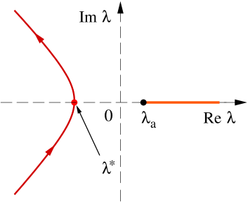
Figure 9: (Color online) Schematic steepest descent contour (in red) for the case when the branch point $\lambda_{\text{a}}$ is not between the origin and the saddle point $\lambda^{*}$. Here, it is shown for $\lambda^{*}<0$, however, one can also have $\lambda^{*}\in(0,\lambda_{\text{a}})$. The direction towards which the contour bends, depends on the value of $w$. Here, it is shown for $w<0$. For $w>0$ the contour bends towards the positive $\mathrm{Re}(\lambda)$ axis, whereas for $w=0$, the steepest descent contour is parallel to the $\mathrm{Im}(\lambda)$ axis. The thick solid (orange) line along the $\mathrm{Re}(\lambda)$ axis from $\lambda_{\text{a}}$ represents the branch cut.

In this case, since $\lambda_{\text{a}}$ lies outside the interval $(0,\lambda^{*})$, one can deform the contour of integration in Eq. (118) into the steepest descent path through $\lambda^{*}$ without hitting $\lambda_{\text{a}}$ (see Fig. 9). Along the steepest descent contour we define

$$f_{w}(\lambda)-f_{w}(\lambda^{*})=-u^{2}.$$ (119)

Therefore, $\lambda_{\text{a}}$ is mapped to a branch point at $u=-ib$ with

$$b=\sqrt{f_{w}(\lambda_{\text{a}})-f_{w}(\lambda^{*})}$$ (120)

and Eq. (118) becomes

$$I=\frac{e^{\tau f_{w}(\lambda^{*})}}{2\pi i}\int_{-\infty}^{\infty}q_{1}(u)\,\frac{e^{-\tau u^{2}}}{\sqrt{b-iu}}\,du$$ (121)

with

$$q_{1}(u)=g_{1}(\lambda)\,\frac{\sqrt{b-iu}}{\sqrt{\lambda_{\text{a}}-\lambda}}\,\frac{d\lambda}{du}.$$ (122)

Now, making a change of variable $\sqrt{\tau}u\rightarrow u$ and taking the large-$\tau$ limit we get

$$I\approx\frac{e^{\tau f_{w}(\lambda^{*})}}{2\pi i}q_{1}(0)\tau^{-1/4}\int_{-\infty}^{\infty}\frac{e^{-u^{2}}}{\sqrt{b\sqrt{\tau}-iu}}\,du,$$ (123)

where

$$q_{1}(0)=g_{1}(\lambda^{*})\,\frac{\sqrt{b}}{\sqrt{\lambda_{\text{a}}-\lambda^{*}}}\,\frac{d\lambda}{du}\bigg{|}_{\lambda\rightarrow\lambda^{*}}.$$ (124)

Using $-u^{2}=\frac{1}{2}f^{\prime\prime}(\lambda^{*})(\lambda-\lambda^{*})^{2}+\dotsb$ as $\lambda\rightarrow\lambda^{*}$, it can be found that

$$\frac{d\lambda}{du}\bigg{|}_{\lambda\rightarrow\lambda^{*}}=\frac{i\sqrt{2}}{\sqrt{f^{\prime\prime}(\lambda^{*})}}\,.$$ (125)

Therefore, we get

$$I\approx\frac{g_{1}(\lambda^{*})}{\sqrt{\lambda_{\text{a}}-\lambda^{*}}}\frac{e^{\tau f_{w}(\lambda^{*})}}{\sqrt{2\pi\tau f^{\prime\prime}_{w}(\lambda^{*})}}\,R_{1}(\sqrt{\tau}\,b),$$ (126)

where

$$R_{1}(z)=\sqrt{\frac{z}{\pi}}\int_{-\infty}^{\infty}\frac{e^{-u^{2}}}{\sqrt{z-iu}}\,du.$$ (127)

We perform this integral in the Mathematica to get Eq. (30).

C.2 The branch point is between the origin and the saddle point: $\lambda_{\text{a}}\in(0,\lambda^{*})$

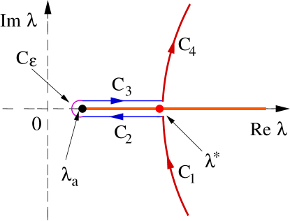
Figure 10: (Color online) Schematic steepest descent contour for the case when the branch point $\lambda_{\text{a}}$ is between the origin and the saddle point $\lambda^{*}$. The thick solid (orange) line along the $\mathrm{Re}(\lambda)$ axis from $\lambda_{\text{a}}$ represents the branch cut. The steepest descent contour goes around the branch cut as shown by $C_{2}$ and $C_{3}$ (in blue). The contribution coming from the circular contour (in magenta) $C_{\epsilon}$ around the branch point becomes zero in the the limit of the radius $\epsilon\rightarrow 0$. The direction towards which the contours $C_{1}$ and $C_{4}$ (shown in red) bend, depends on the value of $w$. Here, it is shown for $w>0$. For $w<0$ the $C_{1}$ and $C_{4}$ bend towards the negative $\mathrm{Re}(\lambda)$ axis, whereas for $w=0$, they are parallel to the $\mathrm{Im}(\lambda)$ axis.

In this case, since $\lambda_{\text{a}}$ lies in the interval $(0,\lambda^{*})$, the deformed contour the through $\lambda^{*}$ wraps around the branch cut. The contour of integration $C=C_{1}+C_{2}+C_{3}+C_{4}+C_{\epsilon}$ is shown in Fig. 10. The contour $C_{\epsilon}$ represents the circular contour of radius $\epsilon$ going around the branch point, and its contribution becomes zero in the limit $\epsilon\rightarrow 0$. The integral in Eq. (118) can be written as $I=P_{\text{B}}+P_{\text{S}},$ where $P_{\text{B}}(w,\tau)$ is the contribution coming from the integrations along the contours $C_{2}$ and $C_{3}$, whereas $P_{\text{S}}$ is the saddle point contribution coming from the integrations along the contours $C_{1}$ and $C_{4}$. In the following we evaluate $P_{\text{B}}$ and $P_{\text{S}}$.

C.2.1 Branch cut contribution

We consider,

$$P_{\text{B}}=\frac{1}{2\pi i}\int_{C_{2}+C_{3}}g_{1}(\lambda)\frac{e^{\tau f_{w}(\lambda)}}{\sqrt{\lambda_{\text{a}}-\lambda}}\,d\lambda.$$ (128)

We note that $\sqrt{\lambda_{\text{a}}-\lambda}$ changes when one goes from $C_{2}$ to $C_{3}$. More precisely, $\lambda_{\text{a}}-\lambda=|\lambda_{\text{a}}-\lambda|e^{i\phi}$, where $\phi=+\pi$ on $C_{2}$ and $\phi=-\pi$ on $C_{3}$ (as $\phi=0$ for $\lambda<\lambda_{\text{a}}$ on the real-$\lambda$ line). Therefore, $\sqrt{\lambda_{\text{a}}-\lambda}=+i|\lambda_{\text{a}}-\lambda|^{1/2}$ on $C_{2}$ and $\sqrt{\lambda_{\text{a}}-\lambda}=-i|\lambda_{\text{a}}-\lambda|^{1/2}$ on $C_{3}$, using which from Eq. (128) we get

$$P_{\text{B}}=\frac{1}{\pi}\int_{\lambda_{\text{a}}}^{\lambda^{*}}g_{1}(\lambda)\frac{e^{\tau f_{w}(\lambda)}}{|\lambda-\lambda_{\text{a}}|^{1/2}}\,d\lambda.$$ (129)

Since $f_{w}(\lambda)$ is real, $f_{w}(\lambda_{\text{a}})>f_{w}(\lambda)>f_{w}(\lambda^{*})$ for $\lambda_{\text{a}}<\lambda<\lambda^{*}$, and $f_{w}(\lambda)$ is minimum at $\lambda^{*}$ along the real $\lambda$ line, we set

$$f_{w}(\lambda)-f_{w}(\lambda_{\text{a}})=-2bu+u^{2}.$$ (130)

The branch point $\lambda_{\text{a}}$ is mapped to $u=0$. Using $f^{\prime}_{w}(\lambda^{*})=0$, we find that the saddle point is mapped to $u=b$, and $b$ can be found by putting $\lambda=\lambda^{*}$ and $u=b$ in the above equation, which gives Eq. (120). With the above mapping from $\lambda$ to $u$, Eq. (128) becomes

$$P_{\text{B}}=\frac{e^{\tau f_{w}(\lambda_{\text{a}})}}{\pi}\int_{0}^{b}q_{2}(u)\frac{e^{-\tau(2bu-u^{2})}}{\sqrt{u}}\,du,$$ (131)

where

$$q_{2}(u)=g_{1}(\lambda)\,\frac{\sqrt{u}}{|\lambda-\lambda_{\text{a}}|^{1/2}}\,\frac{d\lambda}{du}.$$ (132)

From Eq. (130), we get

$$\frac{d\lambda}{du}=\frac{2(u-b)}{f^{\prime}_{w}(\lambda)},$$ (133)

which is finite and nonzero everywhere between $u=0$ and $u=b$. Near $u=0$ we get

$$\left.\frac{d\lambda}{du}\right|_{u=0}=\frac{2b}{-f^{\prime}_{w}(\lambda_{\text{a}})}.$$ (134)

On the other hand, near $u=b$, by applying L’Hospital rule to Eq. (133) we get

$$\left.\frac{d\lambda}{du}\right|_{u=b}=\frac{\sqrt{2}}{\sqrt{f^{\prime\prime}_{w}(\lambda^{*})}}.$$ (135)

Now, making a change of variable $\sqrt{\tau}u\rightarrow u$ in Eq. (131) and then taking the large-$\tau$ limit we get

$$P_{\text{B}}\approx\frac{e^{\tau f_{w}(\lambda_{\text{a}})}}{\pi}\frac{q_{2}(0)}{\tau^{1/4}}R_{2}(\sqrt{\tau}b),$$ (136)

where

$$R_{2}(z)=\int_{0}^{z}\frac{1}{\sqrt{u}}\,e^{-2zu+u^{2}}\,du.$$ (137)

The asymptotic forms of $R_{2}(z)$ can be easily determined from the above integral, which gives $R_{2}(z)\sim\sqrt{\pi}/\sqrt{2z}$ as $z\rightarrow\infty$.

It can be shown that

$$\frac{\sqrt{u}}{|\lambda-\lambda_{\text{a}}|^{1/2}}\,\frac{d\lambda}{du}\xrightarrow[\lambda\rightarrow\lambda_{\text{a}}]{u\rightarrow 0}\Biggl{[}\frac{d\lambda}{du}\bigg{|}_{u=0}\Biggr{]}^{1/2}.$$ (138)

Therefore,

$$q_{2}(0)=g_{1}(\lambda_{\text{a}})\,\Biggl{[}\frac{d\lambda}{du}\bigg{|}_{u=0}\Biggr{]}^{1/2}.$$ (139)

C.2.2 Saddle point contribution

We consider,

$$P_{\text{S}}=\frac{1}{2\pi i}\int_{C_{1}+C_{4}}g_{1}(\lambda)\frac{e^{\tau f_{w}(\lambda)}}{\sqrt{\lambda_{\text{a}}-\lambda}}\,d\lambda.$$ (140)

We make a transform from $\lambda$ to $u$ as defined by Eq. (119). In this case, the branch point $\lambda_{\text{a}}$ is mapped to a branch point at $u=ib$ where $b$ is given by Eq. (120), and Eq. (140) becomes

$$P_{\text{S}}=\frac{e^{\tau f_{w}(\lambda^{*})}}{2\pi i}\int_{-\infty}^{\infty}q_{3}(u)\,\frac{e^{-\tau u^{2}}}{\sqrt{b+iu}}\,du$$ (141)

with

$$q_{3}(u)=g_{1}(\lambda)\,\frac{\sqrt{b+iu}}{\sqrt{\lambda_{\text{a}}-\lambda}}\,\frac{d\lambda}{du}.$$ (142)

We found in the preceding sub-subsection that $\sqrt{\lambda_{\text{a}}-\lambda^{*}}=\pm i|\lambda_{\text{a}}-\lambda^{*}|^{1/2}$ below ($+$) and above ($-$) the branch cut respectively. Therefore, $q_{3}(u)$ approaches two different limits as $u\rightarrow 0$ form above ($0^{+}$) and below ($0^{-}$) respectively:

$$q_{3}(0^{\pm})=\mp\frac{g_{1}(\lambda^{*})\sqrt{b}}{|\lambda_{\text{a}}-\lambda^{*}|^{1/2}}\frac{\sqrt{2}}{\sqrt{f^{\prime\prime}(\lambda^{*})}}\,,$$ (143)

where we have used Eq. (125) for the Jacobian. Thus, upon changing $\sqrt{\tau}u\rightarrow u$ and taking the large-$\tau$ limit yields

$$P_{\text{S}}\approx\frac{g_{1}(\lambda^{*})}{|\lambda_{\text{a}}-\lambda^{*}|^{1/2}}\frac{e^{\tau f_{w}(\lambda^{*})}}{\sqrt{2\pi\tau f^{\prime\prime}(\lambda^{*})}}\,R_{4}(\sqrt{\tau}\,b),$$ (144)

where

$$R_{4}(z) =\sqrt{\frac{z}{\pi}}\left[\int_{0}^{\infty}\frac{e^{-u^{2}}\,du}{\sqrt{z+iu}}-\int_{-\infty}^{0}\frac{e^{-u^{2}}\,du}{\sqrt{z+iu}}\right]i$$

$$=\sqrt{\frac{z}{\pi}}\int_{0}^{\infty}du\,e^{-u^{2}}\left[\frac{1}{\sqrt{z+iu}}-\frac{1}{\sqrt{z-iu}}\right]i.$$ (145)

We evaluate this integral in Mathematica to get Eq. (37), where the generalized hypergeometric function has the series expansion

$${}_{2}F_{2}(a_{1},a_{2};b_{1},b_{2};z)=\sum_{n=0}^{\infty}\frac{\left(a_{1}\right)_{n}\left(a_{2}\right)_{k}}{\left(b_{1}\right)_{k}\left(b_{2}\right)_{n}}\frac{z^{n}}{n!}$$ (146)

with $(a)_{n}=a(a+1)(a+2)\cdots(a+n-1)$, $(a)_{0}=1$ being the the Pochhammer symbol.

The large $z$ behavior of $R_{4}(z)$ can be found by expanding the term inside the square bracket in Eq. (145) in powers of $1/z$ and integrating term by term. This gives $R_{4}(z)\simeq 1/(2\sqrt{\pi}\,z)$ for large $z$.

On the other hand, $R_{4}(z)\simeq\Gamma(1/4)\sqrt{z/2\pi}$ for small $z$. Using this together with $\lim_{\lambda^{*}\rightarrow\lambda_{\text{a}}}\sqrt{b}/|\lambda_{\text{a}}-\lambda^{*}|^{1/2}=[f^{\prime\prime}(\lambda^{*})/2]^{1/4}$ in Eq. (144) we get

$$P_{\text{S}}\approx\frac{\Gamma(1/4)}{2\pi}\frac{g_{1}(\lambda^{*})e^{\tau f_{w}(\lambda^{*})}}{[2\tau f^{\prime\prime}_{w}(\lambda^{*})]^{1/4}}\,\quad\text{as}~{}\lambda^{*}\rightarrow\lambda_{\text{a}}.$$ (147)

Appendix D Index of the notations

• $\gamma$ is the viscous drag.

• $k$ is the stiffness (spring constant) of the trap.

• $D=k_{B}T/\gamma$ is the diffusion constant.

• $\tau_{\gamma}=\gamma/k$ is the viscous relaxation time of the trap, which is introduced in Eq. (1).

• $\tau_{0}$ is the correlation time of trap modulation, which is introduced in Eq. (2).

• $\tau_{c}$ is defined in Eq. (11).

• $\theta$ and $\delta$ are given by Eq. (4).

• $\alpha$ is defined by Eq. (5), and related to $\theta$ and $\delta$ by Eq. (6).

• $a$ is defined in Eq. (12).

• $\mu(\lambda)$ is given by Eq. (11).

• $\nu(\lambda)$ is given by Eq. (12) and Eq. (23).

• $g(\lambda)$ is given by Eq. (16).

• $f_{w}(\lambda)$ is defined in Eq. (20).

• $b_{\pm}$ are defined by Eq. (17).

• $\lambda_{\pm}$ are defined by Eq. (22).

• $\lambda^{*}$ is given by Eq. (21).

• $\lambda_{i}$ with $i\in\{\text{a},\text{b},\text{c},\text{d}\}$, are the positions of the branch points of $g(\lambda)$ and are given by Eqs. (103)–(106).

• $h_{s}(w)=f_{w}(\lambda^{*})$ is given by Eq. (25).

• $h_{i}(w)=f_{w}(\lambda_{i})$ with $i\in\{\text{a},\text{b},\text{c},\text{d}\}$, are given by Eqs. (108)–(111).

• $w^{*}_{i}$ with $i\in\{\text{a},\text{b},\text{c},\text{d}\}$, are given by Eq. (113).

• $\widetilde{g}(\lambda_{i})$ with $i\in\{\text{a},\text{b},\text{c},\text{d}\}$, are defined by Eq. (112).

• $\theta_{c_{1}}$, $\theta_{c_{2}}$, and $\theta_{c}$ are given by Eqs. (114), (116), and (64) respectively.