Training Support Vector Machines Using Frank-Wolfe Optimization Methods

Abstract

Training a Support Vector Machine (SVM) requires the solution of a quadratic programming problem (QP) whose computational complexity becomes prohibitively expensive for large scale datasets. Traditional optimization methods cannot be directly applied in these cases, mainly due to memory restrictions.

By adopting a slightly different objective function and under mild conditions on the kernel used within the model, efficient algorithms to train SVMs have been devised under the name of Core Vector Machines (CVMs). This framework exploits the equivalence of the resulting learning problem with the task of building a Minimal Enclosing Ball (MEB) problem in a feature space, where data is implicitly embedded by a kernel function.

In this paper, we improve on the CVM approach by proposing two novel methods to build SVMs based on the Frank-Wolfe algorithm, recently revisited as a fast method to approximate the solution of a MEB problem. In contrast to CVMs, our algorithms do not require to compute the solutions of a sequence of increasingly complex QPs and are defined by using only analytic optimization steps. Experiments on a large collection of datasets show that our methods scale better than CVMs in most cases, sometimes at the price of a slightly lower accuracy. As CVMs, the proposed methods can be easily extended to machine learning problems other than binary classification. However, effective classifiers are also obtained using kernels which do not satisfy the condition required by CVMs and can thus be used for a wider set of problems.

1 Introduction

Support Vector Machines (SVMs) are currently one of the most effective methods to approach classification and other machine learning problems, improving on more traditional techniques like decision trees and neural networks in a number of applications [16, 33]. SVMs are defined by optimizing a regularized risk functional on the training data, which in most cases leads to classifiers with an outstanding generalization performance [39, 33]. This optimization problem is usually formulated as a large convex quadratic programming problem (QP), for which a naive implementation requires $O(m^{2})$ space and $O(m^{3})$ time in the number of examples $m$, complexities that are prohibitively expensive for large scale problems [33, 37]. Major research efforts have been hence directed towards scaling up SVM algorithms to large datasets.

Due to the typically dense structure of the hessian matrices involved in the QP, traditional optimization methods cannot be directly applied to train an SVM on large datasets. The problem is usually addressed using an active set method where at each iteration only a small number of variables are allowed to change [32, 18, 30]. In non-linear SVMs problems, this is essentially equivalent to selecting a subset of training examples called a working set [39]. The most prominent example in this category of methods is Sequential Minimal Optimization (SMO), where only two variables are selected for optimization each time [8, 30]. The main disadvantage of these methods is that they generally exhibit a slow local rate of convergence, that is, the closer one gets to a solution, the more slowly one approaches that solution. Moreover, performance results are in practice very sensitive to the size of the active set, the way to select the active variables and other implementation details like the caching strategy used to avoid repetitive computations of the kernel function on which the model is based [32] Other attempts to scale up SVM methods consist in adapting interior point methods to some classes of the SVM QP.[9]. For large-scale problems however the resulting rank of the kernel matrix can still be too high to be handled efficiently [37]. The reformulation of the SVM objective function as in [12], the use of sampling methods to reduce the number of variables in the problem as in [22] and [20], and the combination of small SVMs using ensemble methods as in [29] have also been explored.

Looking for more efficient methods, in [37] a new approach was proposed: the task of learning the classifier from data can be transformed to the problem of computing a minimal enclosing ball (MEB), that is, the ball of smallest radius containing a set of points. This equivalence is obtained by adopting a slightly different penalty term in the objective function and imposing some mild conditions on the kernel used by the SVM. Recent advances in computational geometry have demonstrated that there are algorithms capable of approximating a MEB with any degree of accuracy $\epsilon$ in $O(1/\epsilon)$ iterations independently of the number of points and the dimensionality of the space in which the ball is built [37]. Adopting one of these algorithms, Tsang and colleagues devised in [37] the Core Vector Machine (CVM), demonstrating that the new method compares favorably with most traditional SVM software, including for example software based on SMO [8, 30].

CVMs start by solving the optimization problem on a small subset of data and then proceed iteratively. At each iteration the algorithm looks for a point outside the approximation of the MEB obtained so far. If this point exists, it is added to the previous subset of data to define a larger optimization problem, which is solved to obtain a new approximation to the MEB. The process is repeated until no points outside the current approximating ball are found within a prescribed tolerance. CVMs hence need the resolution of a sequence of optimization problems of increasing complexity using an external numerical solver. In order to be efficient, the solver should be able to solve each problem from a warm-start and to avoid the full storage of the corresponding Gram matrix. Experiments in Ref. 37 employ to this end a variant of the second-order SMO proposed in [8].

In this paper, we study two novel algorithms that exploit the formalism of CVMs but do not need the resolution of a sequence of QPs. These algorithms are based on the Frank-Wolfe (FW) optimization framework, introduced in [11] and recently studied in [41] and [4] as a method to approximate the solution of the MEB problem and other convex optimization problems defined on the unit simplex. Both algorithms can be used to obtain a solution arbitrarily close to the optimum, but at the same time are considerably simpler than CVMs. The key idea is to replace the nested optimization problem to be solved at each iteration of the CVM approach by a linearization of the objective function at the current feasible solution and an exact line search in the direction obtained from the linearization. Consequently, each iteration becomes fairly cheaper than a CVM iteration and does not require any external numerical solver.

Similar to CVMs, both algorithms incrementally discover the examples which become support vectors in the SVM model, looking for the optimal set of weights in the process. However, the second of the proposed algorithms is also endowed with the ability to explicitly remove examples from the working set used at each iteration of the procedure and has thus the potential to compute smaller models. On the theoretical side, both algorithms are guaranteed to succeed in $O(1/\epsilon)$ iterations for an arbitrary $\epsilon>0$. In addition, the second algorithm exhibits an asymptotically linear rate of convergence [41].

This research was originally motivated by the use of the MEB framework and computational geometry optimization for the problem of training an SVM. However, a major advantage of the proposed methods over the CVM approach is the possibility to employ kernels which do not satisfy the conditions required to obtain the equivalence between the SVM and MEB optimization problems. For example, the popular polynomial kernel does not allow the use of CVMs as a training method. Since the optimal kernel for a given application cannot be specified a priori, the capability of a training method to work with any valid kernel function is an important feature. Adaptations of the CVM to handle more general kernels have been recently proposed in [38] but, in contrast, our algorithms can be used with any Mercer kernel without changes to the theory or the implementation.

The effectiveness of the proposed methods is evaluated on several data classification sets, most of them already used to show the improvements of CVMs over second-order SMO [37]. Our experimental results suggest that, as long as a minor loss in accuracy is acceptable, our algorithms significantly improve the actual running times of this algorithm. Statistical tests are conducted to assess the significance of these conclusions. In addition, our experiments confirm that effective classifiers are also obtained with kernels that do not fulfill the conditions required by CVMs.

The article is organized as follows. Section $2$ presents a brief overview on SVMs and the way by which the problem of computing an SVM can be treated as a MEB problem. Section $3$ describes the CVM approach. In Section $4$ we introduce the proposed methods. Section $5$ presents the experimental setting and our numerical results. Section $6$ closes the article with a discussion of the main conclusions of this research.

2 Support Vector Machines and the MEB Equivalence

In this section we present an overview on Support Vector Machines (SVMs), and discuss the conditions under which the problem of building these models can be treated as a Minimal Enclosing Ball (MEB) problem in a feature space.

2.1 The Pattern Classification Problem

Consider a set of training data $S=\{\mathbf{x}_{i}\}$ with $\mathbf{x}_{i}\in\mathcal{X}$, $i\in\mathcal{I}=\{1,\ldots,m\}$. The set $\mathcal{X}$, often coinciding with $\mathbb{R}^{n}$, is called the input space, and each instance is associated with a given category in the set $C=\{c_{1},c_{2},\ldots,c_{K}\}$. A pattern classification problem consists of inferring from $S$ a prediction mechanism $f:\mathcal{X}\rightarrow C\in\mathcal{F}$, termed hypothesis, to associate new instances $\mathbf{x}\in\mathcal{X}$ with the correct category. When $K=2$ the problem described above is called binary classification. This problem can be addressed by defining a set of candidate models $\mathcal{F}$, a risk functional $R_{l}(S,f)$ assessing the ability of $f$ to correctly predict the category of the instances in $\mathcal{X}$, and a procedure $L$ by which a dataset $S$ is mapped to a given hypothesis $f=L(S)\in\mathcal{F}$ achieving a low risk. In the context of machine learning, $L$ is called the learning algorithm, $\mathcal{F}$ the hypothesis space and $R_{l}(S,f)$ the induction principle [33].

In the rest of this paper we focus on the problem of computing a model designed for binary classification problems. The extension of these models to handle multiple categories can be accomplished in several ways. A possible approach corresponds to use several binary classifiers, separately trained and joined into a multi-category decision function. Well known approaches of this type are one-versus-the-rest (OVR, see [39]), where one classifier is trained to separate each class from the rest; one-versus-one (OVO, see [19]), where different binary SVMs are used to separate each possible pair of classes; and DDAG, where one-versus-one classifiers are organized in a directed acyclic graph decision structure [33]. Previous experiments with SVMs show that OVO frequently obtains a better performance both in terms of accuracy and training time [17]. Another type of extension consists in reformulating the optimization problem underlying the method to directly address multiple categories. See [6], [23], [28] and [1] for details about these methods.

2.2 Linear Classifiers and Kernels

Support Vector Machines implement the decision mechanism by using simple linear functions. Since in realistic problems the configuration of the data can be highly non-linear, SVMs build a linear model not in the original space $\mathcal{X}$, but in a high-dimensional dot product feature space $\mathcal{P}=\overline{\mbox{lin}\left(\phi(\mathcal{X})\right)}$ where the original data is embedded through the mapping $\mathbf{p}=\phi(\mathbf{x})$ for each $\mathbf{x}\in\mathcal{X}$. In this space, it is expected that an accurate decision function can be linearly represented. The feature space is related with $\mathcal{X}$ by means of a so called kernel function $k:\mathcal{X}\times\mathcal{X}\rightarrow\mathbb{R}$, which allows to compute dot products in $\mathcal{P}$ directly from the input space. More precisely, for each $\mathbf{x}_{i}$, $\mathbf{x}_{j}$ $\in\mathcal{X}$, we have $\mathbf{p}_{i}^{T}\mathbf{p}_{j}=k(\mathbf{x}_{i},\mathbf{x}_{j})$. The explicit computation of the mapping $\phi$, which would be computationally infeasible, is thus avoided [33]. For binary classification problems, the most common approach is to associate a positive label $y_{i}=+1$ to the examples of the first class, and a negative label $y_{i}=-1$ to the examples belonging to the other class. This approach allows the use of real valued hypotheses $h:\mathcal{P}\rightarrow\mathbb{R}$, whose output is passed through a sign threshold to yield the classification label $f(\mathbf{x})=\mbox{sgn}(h(\mathbf{p}))=\mbox{sgn}(h(\phi(\mathbf{x})))$. Since $h(\mathbf{p})$ is a linear function in $\mathcal{P}$, the final prediction mechanism takes the form

$$f(\mathbf{x})=\mbox{sgn}\left(h(\phi(\mathbf{x}))\right)=\mbox{sgn}\left(\mathbf{w}^{T}\phi(\mathbf{x})+b\right)\,,$$ (1)

with $\mathbf{w}\in\mathcal{P}$ and $b\in\mathbb{R}$. This gives a classification rule whose decision boundary $H=\{\mathbf{p}:\mathbf{w}^{T}\mathbf{p}+b=0\}$ is a hyperplane with normal vector $\mathbf{w}$ and position parameter $b$.

2.3 Large Margin Classifiers

It should be noted that a decision function well predicting the training data does not necessarily classify well unseen examples. Hence, minimizing the training error (or empirical risk)

$$\sum_{i\in\mathcal{I}}\frac{1}{2}\left|1-y_{i}f(\mathbf{x}_{i})\right|\,,$$ (2)

does not necessarily imply a small test error. The implementation of an induction principle $R_{l}(S,f)$ guaranteeing a good classification performance on new instances of the problem is addressed in SVMs by building on the concept of margin $\rho$. For a given training pair $\mathbf{x}_{i},y_{i}$, the margin is defined as $\rho_{i}=\rho_{f}(\mathbf{x}_{i},y_{i})=y_{i}h(\mathbf{x}_{i})=y_{i}\left(\mathbf{w}^{T}\phi(\mathbf{x})+b\right)$ and is expected to estimate how reliable the prediction of the model on this pattern is. Note that the example $\mathbf{x}_{i}$ is misclassified if and only if $\rho_{i}<0$. Note also that a large margin of the pattern $\mathbf{x}_{i}$ suggests a more robust decision with respect to changes in the parameters of the decision function $f(\mathbf{x})$, which are to be estimated from the training sample [33]. The margin attained by a given prediction mechanism on the full training set $S$ is defined as the minimum margin over the whole sample, that is $\rho=\min_{i\in\mathcal{I}}\rho_{f}(\mathbf{x}_{i},y_{i})$. This implements a measure of the worst classification performance on the training set, since $\rho_{i}\geq\rho$ $\forall\,i$ [35]. Under some regularity conditions, a large margin leads to theoretical guarantees of good performance on new decision instances [39]. The decision function maximizing the margin on the training data is thus obtained by solving

$$\operatorname*{maximize}_{\mathbf{w},b}\rho=\operatorname*{maximize}_{\mathbf{w},b}\min_{i}\rho_{f}(\mathbf{x}_{i},y_{i})\,.$$ (3)

or, equivalently,

$$\operatorname*{maximize}_{\mathbf{w},b} \;\;\rho$$ (4)

subject to $$\;\;\rho_{i}\geq\rho,\;\;i\in\mathcal{I}\,.$$

However, without some constraint on the size of $\mathbf{w}$, the solution to this maximin problem does not exist [35, 14]. On the other hand, even if we fix the norm of $\mathbf{w}$, a separating hyperplane guaranteeing a positive margin $\rho_{f}(\mathbf{x}_{i},y_{i})$ on each training pattern need not exist. This is the case, for example, if a high noise level causes a large overlap of the classes. In this case, the hyperplane maximizing (3) performs poorly because the prediction mechanism is determined entirely by misclassified examples and the theoretical results guaranteeing a good classification accuracy on unseen patterns no longer hold [35]. A standard approach to deal with noisy training patterns is to allow for the possibility of examples violating the constraint $\rho_{i}\geq\rho$ $\forall\,i$ and by computing the margin on a subset of training examples. The exact way by which SVMs address these problems gives rise to specific formulations, called soft-margin SVMs.

2.4 Soft-Margin SVM Formulations

In $L_{1}$-SVMs (see e.g. [5, 33, 14]), degeneracy of problem (3) is addressed by scaling the constraints $\rho_{i}\geq\rho$ as $\tfrac{\rho_{i}}{\|\mathbf{w}\|}\geq\rho$ and by adding the constraint $\|\mathbf{w}\|=\tfrac{1}{\rho}$, so that the problem now takes the form of the quadratic programming problem

$$\operatorname*{minimize}_{\mathbf{w},b} \;\;\tfrac{1}{2}\|\mathbf{w}\|^{2}$$ (5)

subject to $$\;\;\rho_{f}(\mathbf{x}_{i},y_{i})\geq 1,\;\;i\in\mathcal{I}\,.$$

Noisy training examples are handled by incorporating slack variables $\xi_{i}\geq 0$ to the constraints in (5) and by penalizing them in the objective function:

$$\operatorname*{minimize}_{\mathbf{w},b,\bm{\xi}} \;\;\tfrac{1}{2}\|\mathbf{w}\|^{2}+C\sum_{i\in\mathcal{I}}\xi_{i}$$ (6)

subject to $$\;\;\rho_{f}(\mathbf{x}_{i},y_{i})\geq 1-\xi_{i},\;\;i\in\mathcal{I}\,.$$

This leads to the so called soft-margin $L_{1}$-SVM. In this formulation, the parameter $C$ controls the trade-off between margin maximization and margin constraints violation.

Several other reformulations of problem (3) can be found in literature. In particular, in some formulations the two–norm of $\bm{\xi}$ is penalized instead of the one–norm. In this article, we are particularly interested in the soft margin $L_{2}$-SVM proposed by Lee and Mangasarian in [24]. In this formulation, the margin constraints $\rho_{i}\geq\rho$ in (3) are preserved, the margin variable $\rho$ is explicitly incorporated in the objective function and degeneracy is addressed by penalizing the squared norms of both $\mathbf{w}$ and $b$,

$$\operatorname*{minimize}_{\mathbf{w},b,\rho,\bm{\xi}} \;\;\tfrac{1}{2}\left(\|\mathbf{w}\|^{2}+b^{2}+C\sum_{i\in\mathcal{I}}\xi_{i}^{2}\right)-\rho$$ (7)

subject to $$\;\;\rho_{f}(\mathbf{x}_{i},y_{i})\geq\rho-\xi_{i},\;\;i\in\mathcal{I}\,.$$

In practice, $L_{2}$-SVMs and $L_{1}$-SVMs usually obtain a similar classification accuracy in predicting unseen patterns [24, 37].

2.5 The Target QP

In this paper we focus on the $L_{2}$-SVM model as described above. The use of this formulation is mainly motivated by efficiency: by adopting the slightly modified functional of Eqn. 7, we can exploit the framework introduced in [37] and solve the learning problem more easily, as we will explain in the next Subsection. As a drawback, the constraints of problem (7) explicitly depend on the images $\mathbf{p}_{i}=\phi(\mathbf{x}_{i})$ of the training examples under the mapping $\phi$. In practice, to avoid the explicit computation of the mapping, it is convenient to derive the Wolfe dual of the problem by incorporating multipliers $\alpha_{i}\geq 0,i\in\mathcal{I}$ and considering its Lagrangian

$$L(\mathbf{w},b,\bm{\xi},\bm{\alpha})=\tfrac{1}{2}\left(\|\mathbf{w}\|^{2}+b^{2}+C\sum_{i\in\mathcal{I}}\xi_{i}^{2}\right)-\rho-\sum_{i\in\mathcal{I}}\alpha_{i}\left(\rho_{f}(\mathbf{x}_{i},y_{i})-\rho+\xi_{i}\right)\,.$$ (8)

From the Karush-Kuhn-Tucker conditions for the optimality of (7) with respect to the primal variables we have (see [5, 33, 14]):

$$\frac{\partial L}{\partial\mathbf{w}}=0 \Leftrightarrow\mathbf{w}=\sum_{i\in\mathcal{I}}\alpha_{i}y_{i}\phi(\mathbf{x}_{i})$$ (9)

$$\frac{\partial L}{\partial b}=0 \Leftrightarrow b=\sum_{i\in\mathcal{I}}\alpha_{i}y_{i}$$

$$\frac{\partial L}{\partial\xi_{i}}=0 \Leftrightarrow\xi_{i}=\frac{\alpha_{i}}{C},\;\;i\in\mathcal{I}$$

$$\frac{\partial L}{\partial\rho}=0 \Leftrightarrow\sum_{i\in\mathcal{I}}\alpha_{i}=1\,.$$

Plugging into the Lagrangian, we have

$$L(\mathbf{w},b,\bm{\xi},\bm{\alpha})=-\frac{1}{2}\sum_{i,j\in\mathcal{I}}\alpha_{i}\alpha_{j}y_{i}y_{j}\left(\mathbf{p}_{i}^{T}\mathbf{p}_{j}+1\right)-\frac{1}{2}\sum_{i\in\mathcal{I}}\frac{\alpha_{i}^{2}}{C}\,.$$ (10)

By definition of Wolfe dual (see [33]), it immediately follows that (7) is equivalent to the following QP:

$$\operatorname*{maximize}_{\bm{\alpha}} \;\;-\sum_{i,j\in\mathcal{I}}\alpha_{i}\alpha_{j}\left(y_{i}y_{j}\mathbf{p}_{i}^{T}\mathbf{p}_{j}+y_{i}y_{j}+\frac{\delta_{ij}}{C}\right)$$ (11)

subject to $$\;\;\sum_{i\in\mathcal{I}}\alpha_{i}=1,\ \,\alpha_{i}\geq 0,\;\;i\in\mathcal{I}\,,$$

where $\delta_{ij}$ is equal to 1 if $i=j$, and 0 otherwise. In contrast to (7), the problem above depends on the training examples images $\mathbf{p}_{i}=\phi(\mathbf{x}_{i})$ only through the dot products $\mathbf{p}_{i}^{T}\mathbf{p}_{j}$. By using the kernel function we can hence obtain a problem defined entirely on the original data

$$\operatorname*{maximize}_{\bm{\alpha}} \;\;\Theta(\bm{\alpha}):=-\sum_{i,j\in\mathcal{I}}\alpha_{i}\alpha_{j}\left(y_{i}y_{j}k(\mathbf{x}_{i},\mathbf{x}_{j})+y_{i}y_{j}+\frac{\delta_{ij}}{C}\right)$$ (12)

subject to $$\;\;\sum_{i\in\mathcal{I}}\alpha_{i}=1,\ \,\alpha_{i}\geq 0,\;\;i\in\mathcal{I}\,.$$

From equations (9), we can also write the decision function (1) in terms of the original training examples as $f(\mathbf{x})=\mbox{sgn}\left(h(\mathbf{x})\right)$, where

$$h(\mathbf{x})=\mathbf{w}^{T}\phi(\mathbf{x})+b=\sum_{i\in\mathcal{I}}\alpha_{i}y_{i}\left(k(\mathbf{x}_{i},\mathbf{x})+1\right)\,.$$ (13)

Note that the decision function above depends only on the subset of training examples for which $\alpha_{i}\neq 0$. These examples are usually called the support vectors of the model [33]. The set of support vectors is often considerably smaller than the original training set.

2.6 Computing SVMs as Minimal Enclosing Balls (MEBs)

Now we explain why the $L_{2}$-SVM formulation introduced in the previous paragraphs can lead to efficient algorithms to extract SVM classifiers from data. As pointed out first in [37] and then generalized in [38], the $L_{2}$-SVM can be equivalently formulated as a MEB problem in a certain feature space, that is, as the computation of the ball of smallest radius containing the image of the dataset under a mapping into a dot product space $\mathcal{Z}$.

Consider the image of the training set $S$ under a mapping $\varphi$, that is, $\varphi(S)=\{\mathbf{z}_{i}=\varphi(\mathbf{x}_{i}):i\in\mathcal{I}\}$. Suppose now that there exists a kernel function $\tilde{k}$ such that $\tilde{k}(\mathbf{x}_{i},\mathbf{x}_{j})=\varphi(\mathbf{x}_{i})^{T}\varphi(\mathbf{x}_{j})$ $\forall\,i,j\in\mathcal{I}$. Denote the closed ball of center $\mathbf{c}\in\mathcal{Z}$ and radius $r\in\mathbb{R}^{+}$ as $\mathcal{B}(\mathbf{c},r)$. The MEB $\mathcal{B}(\mathbf{c}^{\ast},r^{\ast})$ of $\varphi(S)$ can be defined as the solution of the following optimization problem

$$\operatorname*{minimize}_{r^{2},\mathbf{c}} \;\ r^{2}$$ (14)

subject to $$\;\ \|\mathbf{z}_{i}-\mathbf{c}\|^{2}\leq r^{2},\;\;i\in\mathcal{I}\,.$$

By using the kernel function $\tilde{k}$ to implement dot products in $\mathcal{Z}$, the following Wolfe dual of the MEB problem is obtained (see [41]):

$$\operatorname*{maximize}_{\bm{\alpha}} \;\ \Phi(\bm{\alpha}):=\sum_{i\in\mathcal{I}}\alpha_{i}\tilde{k}(\mathbf{x}_{i},\mathbf{x}_{i})-\sum_{i,j\in\mathcal{I}}\alpha_{i}\alpha_{j}\tilde{k}(\mathbf{x}_{i},\mathbf{x}_{j})$$ (15)

subject to $$\;\ \sum_{i\in\mathcal{I}}\alpha_{i}=1,\ \,\alpha_{i}\geq 0,\;\;i\in\mathcal{I}\,.$$

If we denote by $\bm{\alpha^{\ast}}$ the solution of (15), formulas for the center $\mathbf{c}^{\ast}$ and the squared radius $r^{\ast 2}$ of MEB$(\varphi(S))$ follow from strong duality:

$$\mathbf{c}^{\ast}=\sum_{i\in\mathcal{I}}\alpha_{i}^{\ast}\mathbf{z}_{i}\,,\;\;r^{\ast 2}=\Phi(\bm{\alpha^{\ast}})=\sum_{i,j\in\mathcal{I}}\alpha_{i}^{\ast}\alpha_{j}^{\ast}\varphi(\mathbf{x}_{i})^{T}\varphi(\mathbf{x}_{j})\,.$$ (16)

Note that the MEB depends only on the subset of points $\mathcal{C}$ for which $\alpha^{\ast}_{i}\neq 0$. It can be shown that computing the MEB on $\mathcal{C}\subset\varphi(S)$ is equivalent to computing the MEB on the entire dataset $\varphi(S)$. This set is frequently called a coreset of $\varphi(S)$, a concept we are going to explore further in the next sections.

We immediately notice a deep similarity between problems (12) and (15), the only difference being the presence of a linear term in the objective function of the latter. This linear term can be neglected under mild conditions on the kernel function $\tilde{k}$. Suppose $\tilde{k}$ fulfills the following normalization condition:

$$\tilde{k}(\mathbf{x}_{i},\mathbf{x}_{i})=\Delta^{2}=\mbox{constant}\,.$$ (17)

Since $\sum_{i\in\mathcal{I}}\alpha_{i}=1$, the linear term $\sum_{i\in\mathcal{I}}\alpha_{i}\tilde{k}(\mathbf{x}_{i},\mathbf{x}_{i})$ in (15) becomes a constant and can be ignored when optimizing for $\bm{\alpha}$. Equivalence between the solutions of problems (12) and (15) follows if we set $\tilde{k}$ to

$$\tilde{k}(\mathbf{x}_{i},\mathbf{x}_{j})=y_{i}y_{j}\left(k(\mathbf{x}_{i},\mathbf{x}_{j})+1\right)+\frac{\delta_{ij}}{C}\,,$$ (18)

where $k$ is the kernel function used within the SVM classifier. Therefore, computing an SVM for a set of labelled data $S=\{\mathbf{x}_{i}:i\in\mathcal{I}\}$ is equivalent to computing the MEB of the set of feature points $\varphi(S)=\{\mathbf{z}_{i}=\varphi(\mathbf{x}_{i}):i\in\mathcal{I}\}$, where the mapping $\varphi$ satisfies the condition $\tilde{k}(\mathbf{x}_{i},\mathbf{x}_{j})=\varphi(\mathbf{x}_{i})^{T}\varphi(\mathbf{x}_{j})$. A possible implementation of such a mapping is $\varphi(\mathbf{x}_{i})=\left(y_{i}\phi(\mathbf{x}_{i}),y_{i},\tfrac{1}{\sqrt{c}}\bm{e}_{i}\right)$, where $\phi(\mathbf{x}_{i})$ is in turn the mapping associated with the original Mercer kernel $k$ used by the SVM.

Note that the previous equivalence between the MEB and the SVM problems holds if and only if the kernel $\tilde{k}$ fulfills assumption (17). If, for example, the SVM classifier implements the well-known $d$-th order polynomial kernel $k(\mathbf{x}_{i},\mathbf{x}_{j})=\left(\mathbf{x}_{i}^{T}\mathbf{x}_{j}+1\right)^{d}$, we have that $\tilde{k}(\mathbf{x}_{i},\mathbf{x}_{i})$ is no longer a constant, and thus the MEB equivalence no longer holds. Complex constructions are required to extend the MEB optimization framework to SVMs using different kernel functions [38].

3 Bădoiu-Clarkson Algorithm and Core Vector Machines

Problem (15) is in general a large and dense QP. Obtaining a numerical solution when $m$ is large is very expensive, no matter which kind of numerical method one decides to employ. Taking into account that in practice we can only approximate the solution within a given tolerance, it is convenient to modify a priori our objective: instead of MEB$(\varphi(S))$, we can try to compute an approximate MEB in the sense specified by the following definition.

Definition 1.

Let MEB$(\varphi(S))$=$\mathcal{B}(\mathbf{c}^{\ast},r^{\ast})$ and $\epsilon>0$ be a given tolerance. Then, a $(1+\epsilon)$–MEB of $\varphi(S)$ is a ball $\mathcal{B}(\mathbf{c},r)$ such that

$$r\leq r^{\ast}\;\;\mbox{and}\;\;\varphi(S)\subset\mathcal{B}(\mathbf{c},(1+\epsilon)r)\,.$$ (19)

A set $\mathcal{C}_{S}\subset\varphi(S)$ is an $\epsilon$–coreset of $\varphi(S)$ if MEB$(\mathcal{C}_{S})$ is a $(1+\epsilon)$–MEB of $\varphi(S)$.

In [2] and [41], algorithms to compute $(1+\epsilon)$–MEBs that scale independently of the dimension of $\mathcal{Z}$ and the cardinality of $S$ have been provided. In particular, the Bădoiu-Clarkson (BC) algorithm described in [2] is able to provide an $\epsilon$–coreset $\mathcal{C}_{S}$ of $\varphi(S)$ in no more than $O(1/\epsilon)$ iterations. We denote with $\mathcal{C}_{k}$ the coreset approximation obtained at the $k$-th iteration and its MEB as $B_{k}=\mathcal{B}(\mathbf{c}_{k},r_{k})$. Starting from a given $\mathcal{C}_{0}$, at each iteration $\mathcal{C}_{k+1}$ is defined as the union of $\mathcal{C}_{k}$ and the point of $\varphi(S)$ furthest from $\mathbf{c}_{k}$. The algorithm then computes $B_{k+1}$ and stops if $\mathcal{B}(\mathbf{c}_{k+1},(1+\epsilon)r_{k+1})$ contains $\varphi(S)$.

Exploiting these ideas, Tsang and colleagues introduced in [37] the CVM (Core Vector Machine) for training SVMs supporting a reduction to a MEB problem. The CVM is described in Algorithm 1, where each $\mathcal{C}_{k}$ is identified by the index set $\mathcal{I}_{k}\subset\mathcal{I}$. The elements included in $\mathcal{C}_{k}$ are called the core vectors. Their role is exactly analogous to that of support vectors in a classical SVM model.

The expression for the radius $r_{k}$ follows easily from (16). Moreover, it is easy to show (see [37]) that step 14 exactly looks for the point $\mathbf{x}_{i^{\ast}}$ whose image $\varphi(\mathbf{x}_{i^{\ast}})$ is the furthest from $\mathbf{c}_{k}$. In fact, by using the expressions $\mathbf{c}_{k}=\sum_{j\in\mathcal{I}_{k}}\alpha_{k,j}\mathbf{z}_{j}$ and $\tilde{k}(\mathbf{x}_{i},\mathbf{x}_{i})=\Delta^{2}$ $\forall\,i\in\mathcal{I}$, we obtain:

$$\|\mathbf{z}_{i}-\mathbf{c}_{k}\|^{2} =\Delta^{2}+\sum_{j,l\in\mathcal{I}_{k}}\alpha_{k,j}\alpha_{k,l}\tilde{k}(\mathbf{x}_{j},\mathbf{x}_{l})-2\sum_{j\in\mathcal{I}_{k}}\alpha_{k,j}\tilde{k}(\mathbf{x}_{j},\mathbf{x}_{i})$$ (20)

$$=\Delta^{2}+R_{k}-2\sum_{j\in\mathcal{I}_{k}}\alpha_{k,j}\tilde{k}(\mathbf{x}_{j},\mathbf{x}_{i})\,.$$

Note how this computation can be performed, by means of kernel evaluations, in spite of the lack of an explicit representation of $\mathbf{c}_{k}$ and $\mathbf{z}_{i}$. Once $i^{\ast}$ has been found, it is included in the index set. Finally, the reduced QP corresponding to the MEB of the new approximate coreset is solved.

Algorithm 1 has two main sources of computational overhead: the computation of the furthest point from $\mathbf{c}_{k}$, which is linear in $m$, and the solution of the optimization subproblem in step 11. The complexity of the former step can be made constant and independent of $m$ by suitable sampling techniques (see [37]), an issue to which we will return later. As regards the optimization step, CVMs adopt a SMO method, where only two variables are selected for optimization at each iteration [8, 30]. It is known that the cost of each SMO iteration is not too high, but the method can require a large number of iterations in order to satisfy reasonable stopping criteria [30].

Algorithm 1 BC Algorithm for MEB-SVMs: the Core Vector Machine

1:$S$, $\epsilon$.

2:initialization: compute $\mathcal{I}_{0}$ and $\bm{\alpha}_{0}$;

3:$\Delta^{2}\longleftarrow\tilde{k}(\mathbf{x}_{1},\mathbf{x}_{1})$;

4:$R_{0}\longleftarrow\sum_{i,j\in\mathcal{I}_{0}}\alpha_{0,i}\alpha_{0,j}\tilde{k}(\mathbf{x}_{i},\mathbf{x}_{j})$;

5:$r_{0}^{2}\longleftarrow\Delta^{2}-R_{0}$;

6:$i^{\ast}\longleftarrow\operatorname*{argmax}_{i\in\mathcal{I}}\gamma^{2}(\bm{\alpha}_{0};i):=\Delta^{2}+R_{0}-2\sum_{j\in\mathcal{I}_{0}}\alpha_{0,j}\tilde{k}(\mathbf{x}_{j},\mathbf{x}_{i})$;

7:$k\longleftarrow 0$;

8:while $\gamma^{2}(\bm{\alpha}_{k};i^{\ast})>(1+\epsilon)^{2}r_{k}^{2}$ do

9:    $k\longleftarrow k+1$;

10:    $\mathcal{I}_{k}\longleftarrow\mathcal{I}_{k-1}\cup\{i^{\ast}\}$;

11:    Find $\bm{\alpha}_{k}$ by solving the reduced QP problem

$$\operatorname*{minimize}_{\bm{\alpha}\in\mathbb{R}^{m}} R(\bm{\alpha}):=\sum_{i,j\in\mathcal{I}_{k}}\alpha_{i}\alpha_{j}\tilde{k}(\mathbf{x}_{i},\mathbf{x}_{j})$$ (21)

subject to $$\sum_{i\in\mathcal{I}_{k}}\alpha_{i}=1,\ \alpha_{i}\geq 0,\;\;i\in\mathcal{I}_{k}\,;$$

12:    $R_{k}\longleftarrow R(\bm{\alpha}_{k})$;

13:    $r_{k}^{2}\longleftarrow\Delta^{2}-R_{k}$;

14:    $i^{\ast}\longleftarrow\operatorname*{argmax}_{i\in\mathcal{I}}\gamma^{2}(\bm{\alpha}_{k};i):=\Delta^{2}+R_{k}-2\sum_{j\in\mathcal{I}_{k}}\alpha_{k,j}\tilde{k}(\mathbf{x}_{j},\mathbf{x}_{i})$;

15:end while

16:return $\mathcal{I}_{S}=\mathcal{I}_{k}$, $\bm{\alpha}=\bm{\alpha}_{k}$.

As regards the initialization, that is, the computation of $\mathcal{C}_{0}$ and $\bm{\alpha}_{0}$, a simple choice is suggested in [21], which consists in choosing $\mathcal{C}_{0}=\{\mathbf{z}_{a},\mathbf{z}_{b}\}$, where $\mathbf{z}_{a}$ is an arbitrary point in $\varphi(S)$ and $\mathbf{z}_{b}$ is the farthest point from $\mathbf{z}_{a}$. Obviously, in this case the center and radius of $B_{0}$ are $\mathbf{c}_{0}=0.5(\mathbf{z}_{a}+\mathbf{z}_{b})$ and $r_{0}=0.5\|\mathbf{z}_{a}-\mathbf{z}_{b}\|$, respectively. That is, we initialize $\mathcal{I}_{0}=\{a,b\}$, $\alpha_{0,a}=\alpha_{0,b}=0.5$ and $\alpha_{0,i}=0$ for $i\notin\mathcal{I}_{0}$. A more efficient strategy, implemented for example in the code LIBCVM [36], is the following. The procedure consists in determining the MEB of a subset $P=\{\mathbf{z}_{i},i\in\mathcal{I}_{P}\}$ of $p$ training points, where the set of indices $\mathcal{I}_{P}$ is randomly chosen and $p$ is small. This MEB is approximated by running a SMO solver. In practice, $p\simeq 20$ is suggested to be enough, but one can also try larger initial guesses, as long as SMO can rapidly compute the initial MEB. $\mathcal{C}_{0}$ is then defined as the set of points $\mathbf{x}_{i}\in P$ gaining a strictly positive dual weight in the process, and $\mathcal{I}_{0}$ as the set of the corresponding indices.

4 Frank-Wolfe Methods for the MEB-SVM Problem

4.1 Overview of the Frank-Wolfe Algorithm

The Frank-Wolfe algorithm (FW), originally presented in [11], is designed to solve optimization problems of the form

$$\operatorname*{maximize}_{\bm{\alpha}\in\Sigma}f(\bm{\alpha})\,,$$ (22)

where $f\in C^{1}(\mathbb{R}^{m})$ is a concave function, and $\Sigma\neq\emptyset$ a bounded convex polyhedron.

In the case of the MEB dual problem, the objective function is quadratic and $\Sigma$ coincides with the unit simplex. Given the current iterate $\bm{\alpha}_{k}\in\Sigma$, a standard Frank-Wolfe iteration consists in the following steps:

1. Find a point $\mathbf{u}_{k}\in\Sigma$ maximizing the local linear approximation $\psi_{k}(\mathbf{u}):=f(\bm{\alpha}_{k})+(\mathbf{u}-\bm{\alpha}_{k})^{T}\nabla f(\bm{\alpha}_{k})$, and define $\mathbf{d}_{k}^{FW}=\mathbf{u}_{k}-\bm{\alpha}_{k}$.

2. Perform a line-search $\lambda_{k}=\operatorname*{argmax}_{\lambda\in[0,1]}f(\bm{\alpha}_{k}+\lambda\mathbf{d}_{k}^{FW})$.

3. Update the iterate by

   $$\bm{\alpha}_{k+1}=\bm{\alpha}_{k}+\lambda_{k}\mathbf{d}_{k}^{FW}=(1-\lambda_{k})\bm{\alpha}_{k}+\lambda_{k}\mathbf{u}_{k}\,.$$ (23)

The algorithm is usually stopped when the objective function is sufficiently close to its optimal value, according to a suitable proximity measure [13].

Since $\psi_{k}(\mathbf{u})$ is a linear function and $\Sigma$ is a bounded polyhedron, the search directions $\mathbf{d}_{k}^{FW}$ are always directed towards an extreme point of $\Sigma$. That is, $\mathbf{u}_{k}$ is a vertex of the feasible set. The constraint $\lambda_{k}\in[0,1]$ ensures feasibility at each iteration. It is easy to show that in the case of the MEB problem $\mathbf{u}_{k}=\mathbf{e}_{i^{\ast}}$, where $\mathbf{e}_{i}$ denotes the $i$-th vector of the canonical basis, and $i^{\ast}$ is the index corresponding to the largest component of $\nabla f(\bm{\alpha}_{k})$ [41]. The updating step therefore assumes the form

$$\bm{\alpha}_{k+1}=(1-\lambda_{k})\bm{\alpha}_{k}+\lambda_{k}\mathbf{e}_{i^{\ast}}\,.$$ (24)

It can be proved that the above procedure converges globally [13]. As a drawback, however, it often exhibits a tendency to stagnate near a solution. Intuitively, suppose that solutions $\bm{\alpha}^{\ast}$ of (22) lie on the boundary of $\Sigma$ (this is often true in practice, and holds in particular for the MEB problem). In this case, as $\bm{\alpha}_{k}$ gets close to a solution $\bm{\alpha}^{\ast}$, the directions $\mathbf{d}_{k}^{FW}$ become more and more orthogonal to $\nabla f(\bm{\alpha}_{k})$. As a consequence, $\bm{\alpha}_{k}$ possibly never reaches the face of $\Sigma$ containing $\bm{\alpha}^{\ast}$, resulting in a sublinear convergence rate [13].

4.2 The Modified Frank-Wolfe Algorithm

We now describe an improvement over the general Frank-Wolfe procedure, which was first proposed in [40] and later detailed in [13]. This improvement can be quantified in terms of the rate of convergence of the algorithm and thus of the number of iterations in which it can be expected to fulfill the stopping conditions.

In practice, the tendency of FW to stagnate near a solution can lead to later iterations wasting computational resources while making minimal progress towards the optimal function value. It would thus be desirable to obtain a stronger result on the convergence rate, which guarantees that the speed of the algorithm does not deteriorate when approaching a solution. This paragraph describes a technique geared precisely towards this aim.

Essentially, the previous algorithm is enhanced by introducing alternative search directions known as away steps. The basic idea is that, instead of moving towards the vertex of $\Sigma$ maximizing a linear approximation $\psi_{k}$ of $f$ in $\bm{\alpha}_{k}$, we can move away from the vertex minimizing $\psi_{k}$. At each iteration, a choice between these two options is made by choosing the best ascent direction. The whole procedure, known as Modified Frank-Wolfe algorithm (MFW), can be sketched as follows:

1. Find $\mathbf{u}_{k}\in\Sigma$ and define $\mathbf{d}_{k}^{FW}$ as in the standard FW algorithm.

2. Find $\mathbf{v}_{k}\in\Sigma$ by minimizing $\psi_{k}(\mathbf{v})$, s.t. $v_{j}=0$ if $\alpha_{k,j}=0$. Define $\mathbf{d}_{k}^{A}=\bm{\alpha}_{k}-\mathbf{v}_{k}$.

3. If $\nabla f(\bm{\alpha}_{k})^{T}\mathbf{d}_{k}^{FW}\geq\nabla f(\bm{\alpha}_{k})^{T}\mathbf{d}_{k}^{A}$, then $\mathbf{d}_{k}=\mathbf{d}_{k}^{FW}$, else $\mathbf{d}_{k}=\mathbf{d}_{k}^{A}$.

4. Perform a line-search $\lambda_{k}=\operatorname*{argmax}_{\lambda\in[0,\bar{\lambda}]}f(\bm{\alpha}_{k}+\lambda\mathbf{d}_{k})$, where $\bar{\lambda}=1$ if $\mathbf{d}_{k}=\mathbf{d}_{k}^{FW}$ and $\bar{\lambda}=\max_{\lambda\geq 0}\left\{\lambda\,|\,\bm{\alpha}_{k}+\lambda\mathbf{d}_{k}^{A}\in\Sigma\right\}$.

5. Update the iterate by

   $$\bm{\alpha}_{k+1}=\bm{\alpha}_{k}+\lambda_{k}\mathbf{d}_{k}=\left\{\begin{aligned} (1-\lambda_{k})\bm{\alpha}_{k}+\lambda_{k}\mathbf{u}_{k}&\qquad\text{if}&\mathbf{d}_{k}&=\mathbf{d}_{k}^{FW}\\ (1+\lambda_{k})\bm{\alpha}_{k}-\lambda_{k}\mathbf{v}_{k}&\qquad\text{if}&\mathbf{d}_{k}&=\mathbf{d}_{k}^{A}\,.\end{aligned}\right.$$ (25)

It is easy to show that both $\mathbf{d}_{k}^{FW}$ and $\mathbf{d}_{k}^{A}$ are feasible ascent directions, unless $\bm{\alpha}_{k}$ is already a stationary point.

In the case of the MEB problem, step 2 corresponds to finding the basis vector $\mathbf{e}_{j^{\ast}}$ corresponding to the smaller component of $\nabla f(\bm{\alpha}_{k})$ [41]. Note that a face of $\Sigma$ of lower dimensionality is reached whenever an away step with maximal stepsize $\bar{\lambda}$ is performed. Imposing the constraint in step 2 is tantamount to ruling out away steps with zero stepsize. That is, an away step from $\mathbf{e}_{j}$ cannot be taken if $\alpha_{k,j}$ is already zero.

In [13] linear convergence of $f(\bm{\alpha}_{k})$ to $f(\bm{\alpha}^{\ast})$ was proved, assuming Lipschitz continuity of $\nabla f$, strong concavity of $f$, and strict complementarity at the solution. In [41], a proof of the same result was provided for the MEB problem, under weaker assumptions. It is important to note that such assumptions are in particular satisfied for the MEB formulation of the $L_{2}$-SVM, and that as such the aforementioned linear convergence property holds for all problems considered in this paper. In particular, uniqueness of the solution, which is implied if we ask for strong (or just strict) concavity, is not required. The gist is essentially that, in a small neighborhood of a solution $\bm{\alpha}^{\ast}$, MFW is forced to perform away steps until the face of $\Sigma$ containing $\bm{\alpha}^{\ast}$ is reached, which happens after a finite number of iterations. Starting from that point, the algorithm behaves as an unconstrained optimization method, and it can be proved that $f(\bm{\alpha}_{k})$ converges to $f(\bm{\alpha}^{\ast})$ linearly [13].

4.3 The FW and MFW Algorithms for MEB-SVMs

If FW method is applied to the MEB dual problem, the structure of the objective function $\Phi(\bm{\alpha})$ can be exploited in order to obtain explicit formulas for steps 1 and 2 of the generic procedure. Indeed, the components of $\nabla\Phi(\bm{\alpha}_{k})$ are given by

$$\nabla\Phi(\bm{\alpha}_{k})_{i}=\|\mathbf{z}_{i}\|^{2}-2\sum_{j\in\mathcal{I}}\alpha_{k,j}\mathbf{z}_{i}^{T}\mathbf{z}_{j}=\|\mathbf{z}_{i}\|^{2}-2\mathbf{z}_{i}^{T}\mathbf{c}_{k}\,,$$ (26)

where

$$\mathbf{c}_{k}=\sum_{j\in\mathcal{I}}\alpha_{k,j}\mathbf{z}_{j}\,,$$ (27)

and therefore, since $\|\mathbf{c}_{k}\|^{2}$ does not depend on $i$,

$$i^{\ast}=\operatorname*{argmax}_{i\in\mathcal{I}}\nabla\Phi(\bm{\alpha}_{k})_{i}=\operatorname*{argmax}_{i\in\mathcal{I}}\|\mathbf{z}_{i}-\mathbf{c}_{k}\|^{2}.$$ (28)

In practice, step 1 selects the index of the input point maximizing the distance from $\mathbf{c}_{k}$, exactly as done in the CVM procedure. Computation of distances can be carried out as in CVMs, using (20). As regards step 2, it can be shown (see [4, 41]) that

$$\lambda_{k}=\frac{1}{2}\left(1-\frac{r_{k}^{2}}{\|\mathbf{z}_{i^{\ast}}-\mathbf{c}_{k}\|^{2}}\right),$$ (29)

where

$$r^{2}_{k}=\Phi(\bm{\alpha}_{k})\,.$$ (30)

By comparing (27) and (30) with (16), we argue that, as in the BC algorithm, a ball $B_{k}=\mathcal{B}(\mathbf{c}_{k},r_{k})$ is identified at each iteration.

The whole procedure is sketched in Algorithm 2, where at each iteration we associate to $\bm{\alpha}_{k}$ the index set $\mathcal{I}_{k}=\{i\in\mathcal{I}:\alpha_{k,i}>0\}$.

Algorithm 2 Frank-Wolfe Algorithm for MEB-SVMs

1:$S$, $\epsilon$.

2:initialization: compute $\mathcal{I}_{0}$ and $\bm{\alpha}_{0}$;

3:$\Delta^{2}\longleftarrow\tilde{k}(\mathbf{x}_{1},\mathbf{x}_{1})$;

4:$R_{0}\longleftarrow\sum_{i,j\in\mathcal{I}_{0}}\alpha_{0,i}\alpha_{0,j}\tilde{k}(\mathbf{x}_{i},\mathbf{x}_{j})$;

5:$r_{0}^{2}\longleftarrow\Delta^{2}-R_{0}$;

6:$i^{\ast}\longleftarrow\operatorname*{argmax}_{i\in\mathcal{I}}\gamma^{2}(\bm{\alpha}_{0};i):=\Delta^{2}+R_{0}-2\sum_{j\in\mathcal{I}_{0}}\alpha_{0,j}\tilde{k}(\mathbf{x}_{j},\mathbf{x}_{i})$;

7:$\delta_{0}\longleftarrow\frac{\gamma^{2}(\bm{\alpha}_{0};i^{\ast})}{r^{2}_{0}}-1$;

8:$k\longleftarrow 0$;

9:while $\delta_{k}>(1+\epsilon)^{2}-1$ do

10:    $\lambda_{k}\longleftarrow\frac{1}{2}\left(1-\frac{r_{k}^{2}}{\gamma^{2}(\bm{\alpha}_{k};i^{\ast})}\right)$;

11:    $k\longleftarrow k+1$;

12:    $\bm{\alpha}_{k}\longleftarrow(1-\lambda_{k-1})\bm{\alpha}_{k-1}+\lambda_{k-1}\mathbf{e}_{i^{\ast}}$;

13:    $\mathcal{I}_{k}\longleftarrow\{i\in\mathcal{I}:\alpha_{k,i}>0\}$;

14:    $R_{k}\longleftarrow\sum_{i,j\in\mathcal{I}_{k}}\alpha_{k,i}\alpha_{k,j}\tilde{k}(\mathbf{x}_{i},\mathbf{x}_{j})$;

15:    $r^{2}_{k}\longleftarrow r^{2}_{k-1}\left(1+\frac{\delta_{k-1}^{2}}{4(1+\delta_{k-1})}\right)$;

16:    $i^{\ast}\longleftarrow\operatorname*{argmax}_{i\in\mathcal{I}}\gamma^{2}(\bm{\alpha}_{k};i):=\Delta^{2}+R_{k}-2\sum_{j\in\mathcal{I}_{k}}\alpha_{k,j}\tilde{k}(\mathbf{x}_{j},\mathbf{x}_{i})$;

17:    $\delta_{k}\longleftarrow\frac{\gamma^{2}(\bm{\alpha}_{k};i^{\ast})}{r^{2}_{k}}-1$;

18:end while

19:return $\mathcal{I}_{S}=\mathcal{I}_{k}$, $\bm{\alpha}=\bm{\alpha}_{k}$.

As regards the initialization, $\bm{\alpha}_{0}$ and $\mathcal{I}_{0}$ can be defined exactly as in the CVM procedure. At subsequent iterations, the formula to update $\mathcal{I}_{k}$ immediately follows from the updating (24) for $\bm{\alpha}_{k}$; indeed, the indices of the strictly positive components of $\bm{\alpha}_{k+1}$ are the same of $\bm{\alpha}_{k}$, plus $i^{\ast}$ if $\alpha_{k,i^{\ast}}=0$ (which means that $\mathbf{z}_{i^{\ast}}$ was not already included in the current coreset). The introduction of the sequence $\{\mathcal{I}_{k}\}$ in Algorithm 2 makes it evident that structure and output of Algorithm 1 are preserved.

The updating formula used in step 15 appears in [41]. It is easy to see that it is equivalent to (30) and computationally more convenient.

In [41], it has been proved that $\{r^{2}_{k}\}$ is a monotonically increasing sequence with $r^{\ast 2}$ as an upper bound. Therefore, since the same stopping criterion of the BC algorithm is used, $\mathcal{I}_{S}$ identifies an $\epsilon$–coreset $\mathcal{C}_{S}$ of $\varphi(S)$, and the last $B_{k}$ is a $(1+\epsilon)$–MEB of $\varphi(S)$. However, the MEB-approximating procedure differs from that of BC in that the value of $r^{2}_{k}$ is not equal to the squared radius of MEB$(\mathcal{C}_{k})$, but tends to the correct value as $\bm{\alpha}_{k}$ gets near the optimal solution (see Fig. 1).

Figure 1: Approximating balls computed by algorithms BC and FW.

The derivation of the MFW method applied to the MEB-SVM problem can be written down along the same lines. Following the presentation in [41], we describe the detailed procedure in Algorithm 3.

Algorithm 3 Modified Frank-Wolfe Algorithm for MEB-SVMs

1:$S$, $\epsilon$.

2:initialization: compute $\mathcal{I}_{0}$ and $\bm{\alpha}_{0}$;

3:$\Delta^{2}\longleftarrow\tilde{k}(\mathbf{x}_{1},\mathbf{x}_{1})$;

4:$R_{0}\longleftarrow\sum_{i,j\in\mathcal{I}_{0}}\alpha_{0,i}\alpha_{0,j}\tilde{k}(\mathbf{x}_{i},\mathbf{x}_{j})$;

5:$r_{0}^{2}\longleftarrow\Delta^{2}-R_{0}$;

6:$i^{\ast}\longleftarrow\operatorname*{argmax}_{i\in\mathcal{I}}\gamma^{2}(\bm{\alpha}_{0};i):=\Delta^{2}+R_{0}-2\sum_{j\in\mathcal{I}_{0}}\alpha_{0,j}\tilde{k}(\mathbf{x}_{j},\mathbf{x}_{i})$;

7:$j^{\ast}\longleftarrow\operatorname*{argmin}_{j\in\mathcal{I}_{0}}\gamma^{2}(\bm{\alpha}_{0};j)$;

8:$\delta_{0+}\longleftarrow\frac{\gamma^{2}(\bm{\alpha}_{0};i^{\ast})}{r^{2}_{k}}-1$;

9:$\delta_{0-}\longleftarrow 1-\frac{\gamma^{2}(\bm{\alpha}_{0};j^{\ast})}{r^{2}_{k}}$;

10:$k\longleftarrow 0$;

11:while  $\delta_{k+}>(1+\epsilon)^{2}-1$ do

12:    if $\delta_{k+}\geq\delta_{k-}$ then

13:         $\lambda_{k}\longleftarrow\frac{1}{2}\left(1-\frac{r_{k}^{2}}{\gamma^{2}(\bm{\alpha}_{k};i^{\ast})}\right)$;

14:         $k\longleftarrow k+1$;

15:         $\bm{\alpha}_{k}\longleftarrow(1-\lambda_{k-1})\bm{\alpha}_{k-1}+\lambda_{k-1}\mathbf{e}_{i^{\ast}}$;

16:         $r^{2}_{k}\longleftarrow r^{2}_{k-1}\left(1+\frac{\delta_{k-1+}^{2}}{4(1+\delta_{k-1+})}\right)$;

17:    else

18:         $\lambda_{k}\longleftarrow\min\left\{\frac{\delta_{k-}}{2(1-\delta_{k-})},\frac{\alpha_{k,{j^{\ast}}}}{1-\alpha_{k,{j^{\ast}}}}\right\}$;

19:         $k\longleftarrow k+1$;

20:         $\bm{\alpha}_{k}\longleftarrow(1+\lambda_{k-1})\bm{\alpha}_{k-1}-\lambda_{k-1}\mathbf{e}_{j^{\ast}}$;

21:         $r^{2}_{k}\longleftarrow(1+\lambda_{k-1})r^{2}_{k-1}-\lambda_{k-1}(1+\lambda_{k-1})(\delta_{k-1-}-1)r^{2}_{k-1}$;

22:    end if

23:    $\mathcal{I}_{k}\longleftarrow\{i\in\mathcal{I}:\alpha_{k,i}>0\}$;

24:    $R_{k}\longleftarrow\sum_{i,j\in\mathcal{I}_{k}}\alpha_{k,i}\alpha_{k,j}\tilde{k}(\mathbf{x}_{i},\mathbf{x}_{j})$;

25:    $i^{\ast}\longleftarrow\operatorname*{argmax}_{i\in\mathcal{I}}\gamma^{2}(\bm{\alpha}_{k};i):=\Delta^{2}+R_{k}-2\sum_{j\in\mathcal{I}_{k}}\alpha_{k,j}\tilde{k}(\mathbf{x}_{j},\mathbf{x}_{i})$;

26:    $j^{\ast}\longleftarrow\operatorname*{argmin}_{j\in\mathcal{I}_{k}}\gamma^{2}(\bm{\alpha}_{k};j)$;

27:    $\delta_{k+}\longleftarrow\frac{\gamma^{2}(\bm{\alpha}_{k};i^{\ast})}{r^{2}_{k}}-1$;

28:    $\delta_{k-}\longleftarrow 1-\frac{\gamma^{2}(\bm{\alpha}_{k};j^{\ast})}{r^{2}_{k}}$;

29:end while

30:return $\mathcal{I}_{S}=\mathcal{I}_{k}$, $\bm{\alpha}=\bm{\alpha}_{k}$.

By now, it should be apparent that $j^{\ast}$ is the index identifying the point furthest from $\mathbf{c}_{k}$, and that it corresponds to the smallest component of $\nabla\Phi(\bm{\alpha}_{k})$. That is, in Algorithm 3 we consider performing away steps in which the weight of the nearest point to the current center is reduced. Of course, since the weight of a point is not allowed to drop below zero, the search for $j^{\ast}$ is performed on $\mathcal{I}_{k}$ only. Again, the optimal stepsize can be determined in closed form [41]. In particular, it is easy to see that the expression in step 20 corresponds to

$$\lambda_{k}=\operatorname*{argmax}_{\lambda\in\left[0,\frac{\alpha_{k,j^{\ast}}}{1-\alpha_{k,j^{\ast}}}\right]}\Phi((1+\lambda)\bm{\alpha}_{k}-\lambda\mathbf{e}_{j^{\ast}})\,,$$ (31)

where the upper bound on the interval preserves dual feasibility.

This kind of step has an intuitive geometrical meaning: if we consider a solution $\bm{\alpha}^{\ast}$ of the MEB problem, it is known that nonzero components of $\bm{\alpha}^{\ast}$ correspond to points lying on the boundary of the exact MEB. Therefore, it makes sense to try to remove from the model points that lie near the center (i.e. far from the boundary of the ball). When an away step is performed, if $\lambda_{k}$ is chosen as the supremum of the search interval, we get $\alpha_{k+1,j^{\ast}}=0$ and the corresponding example is removed from the current coreset (drop step). Moreover, it’s not hard to see that step 12 chooses to perform an away step whenever

$$\nabla\Phi(\bm{\alpha}_{k})^{T}\mathbf{d}^{A}_{k}>\nabla\Phi(\bm{\alpha}_{k})^{T}\mathbf{d}^{FW}_{k}.$$ (32)

That is, the choice between FW and away steps is done by choosing the best ascent direction, exactly as required by the MFW procedure. Here $\mathbf{d}_{k}^{FW}=(\mathbf{e}_{i^{\ast}}-\bm{\alpha}_{k})$ and $\mathbf{d}_{k}^{A}=(\bm{\alpha}_{k}-\mathbf{e}_{j^{\ast}})$ denote the search directions of FW and away steps, respectively. Finally, step 21 shows that, just as with standard FW steps, after performing an away step we can use an analytical formula to update $r^{2}_{k}$. This expression follows easily by writing the objective function $\Phi(\bm{\alpha})$ for $\bm{\alpha}=(1+\lambda)\bm{\alpha}_{k}-\lambda\mathbf{e}_{j^{\ast}}$.

In Fig. 2, we try to give a geometrical insight on the difference between FW and away steps in terms of search directions.

Figure 2: A sketch of the search directions used by FW and MFW.

We previously hinted at the linear convergence properties of MFW. This result can now be stated more precisely [41].

Proposition 1.

At each iteration of the MFW algorithm, we have:

$$\frac{\Phi(\bm{\alpha})-\Phi(\bm{\alpha}_{k+1})}{\Phi(\bm{\alpha})-\Phi(\bm{\alpha}_{k})}\leq M\,,$$ (33)

where $M\leq 1-\frac{1}{36m\beta d_{S}}$, $\beta$ is a constant and $d_{S}=\operatorname*{diam}(S)^{2}$.

Substantially, as shown in the convergence analysis of [13], there exists a point in the optimization path of the MFW algorithm after which only away steps are performed. That is, the algorithm only needs to remove useless examples to correctly identify the optimal support vector set. From this stage on, the algorithm converges linearly to the optimum value of the objective function. In contrast, the standard FW algorithm does not possess the explicit ability to eliminate spurious patterns from the index set, and tends to slow down when getting near the solution.

4.4 Beyond Normalized Kernels

The methods studied in this paper were originally motivated by recent advances in computational geometry that led to efficient algorithms to address the MEB problem [41]. However, a major advantage of the proposed methods, over e.g. the CVM approach, is that both the theory and the implementation of our algorithms can be applied without changes to train SVMs using kernels which do not satisfy condition (17), imposed to obtain the equivalence between the MEB problem (15) and the SVM optimization problem (12).

Both the FW and MFW methods were designed to maximize any differentiable concave function $f(\bm{\alpha})$ in a bounded convex polyhedron. The objective function in the SVM problem (12) is concave and the set of constraints coincides with the unit simplex. The proposed methods can thus be applied directly to solve (12) without regard to (15). Theoretical results such as the global convergence of algorithms still hold. In addition, since strict complementarity usually holds for SVM problems, results in [13] imply that MFW still converges linearly to the optimum. Note also that the constant $\Delta^{2}$, which makes the difference between (15) and (12) for normalized kernels, can still be added to the objective function of (12) in the case of non-normalized kernels, since it is simply ignored when optimizing for $\bm{\alpha}$. An implementation designed to handle normalized kernels can thus be directly used with any Mercer kernel.

It is apparent that the geometrical interpretation underlying Algorithms 2 and 3 needs to be reformulated if the SVM problem is no longer equivalent to the problem of computing a MEB. However, it is easy to show that the search direction of the FW procedure at iteration $k$ is still $\mathbf{e}_{i^{\ast}}$ where the index $i^{\ast}$ corresponds to the largest component of $\nabla f(\bm{\alpha}_{k})$. Similarly, the away direction explored by MFW at iterate $k$ is still $\mathbf{e}_{j^{\ast}}$ where the index $j^{\ast}$ corresponds to the smallest component of $\nabla f(\bm{\alpha}_{k})$. The set of constraints in problem (12) coincides with that of (15). In addition, any approximate solution $\bm{\alpha}_{k}$ produced by the proposed algorithms is feasible. Thus, the sequence $f(\bm{\alpha}_{k})$ is strictly increasing and converges from below to the optimum $f(\bm{\alpha}^{\ast})$. It is not immediately evident, however, whether the stopping condition used within our algorithms guarantees the method to find a solution in a neighborhood of the optimum $\bm{\alpha}_{k}^{*}$. We now show that this is indeed the case. For simplicity of notation, it is convenient to write explicitly the target QP of MEB-SVMs in matrix form:

$$\operatorname*{maximize}_{\bm{\alpha}} \;\;g(\bm{\alpha}):=\Delta^{2}-\bm{\alpha}\tilde{\bm{K}}\bm{\alpha}=\Delta^{2}-\|\mathbf{c}\|^{2}$$ (34)

subject to $$\;\;\mathbf{e}^{T}\bm{\alpha}=1,\;\;\bm{\alpha}\geq 0\,,$$

where $\tilde{\bm{K}}$ is the matrix of entries $\tilde{k}_{ij}=\varphi(\mathbf{x}_{i})^{T}\varphi(\mathbf{x}_{j})=y_{i}y_{j}k(\mathbf{x}_{i},\mathbf{x}_{j})+y_{i}y_{j}+\frac{\delta_{ij}}{C}$, $\mathbf{c}=\bm{Z}\bm{\alpha}$, and $\bm{Z}$ is the matrix whose columns are the feature vectors $\mathbf{z}_{i}=\varphi(\mathbf{x}_{i})$. Note that $\bm{K}=\bm{Z}^{T}\bm{Z}$. When $k$ is a normalized kernel, we get $\Phi(\bm{\alpha})=g(\bm{\alpha})$. For non-normalized kernels, instead, $\Delta^{2}$ can be viewed as an arbitrary constant added to the SVM objective function in (12), $\Theta(\bm{\alpha})=-\bm{\alpha}\tilde{\bm{K}}\bm{\alpha}$. That is, we can always think of $g(\bm{\alpha})$ as the objective function when solving (12).

It is not hard to see that the stopping condition used in Algorithms 2 and 3 can be written as follows:

$$\delta_{k+}\leq(1+\epsilon)^{2}-1$$ (35)

$$\Longleftrightarrow \|\mathbf{z}_{i^{\ast}}-\mathbf{c}_{k}\|^{2}\leq(1+\epsilon)^{2}r_{k}^{2}$$

$$\Longleftrightarrow \Delta^{2}-2\mathbf{z}_{i^{\ast}}^{T}\mathbf{c}_{k}+\|\mathbf{c}_{k}\|^{2}\leq(1+\epsilon)^{2}r_{k}^{2}\,.$$

Since by construction $r_{k}^{2}=\Delta^{2}-\|\mathbf{c}_{k}\|^{2}$, we get

$$\Delta^{2}-2\mathbf{z}_{i^{\ast}}^{T}\mathbf{c}_{k}+\|\mathbf{c}_{k}\|^{2}\leq(1+2\epsilon+\epsilon^{2})\left(\Delta^{2}-\|\mathbf{c}_{k}\|^{2}\right)$$ (36)

$$\Longleftrightarrow \Delta^{2}-2\mathbf{z}_{i^{\ast}}^{T}\mathbf{c}_{k}+\|\mathbf{c}_{k}\|^{2}\leq(1+\varepsilon)\left(\Delta^{2}-\|\mathbf{c}_{k}\|^{2}\right)$$

$$\Longleftrightarrow \Delta^{2}-2\mathbf{z}_{i^{\ast}}^{T}\mathbf{c}_{k}+\|\mathbf{c}_{k}\|^{2}\leq\Delta^{2}-\|\mathbf{c}_{k}\|^{2}+\varepsilon g(\bm{\alpha}_{k})$$

$$\Longleftrightarrow -2\mathbf{z}_{i^{\ast}}^{T}\mathbf{c}_{k}+2\|\mathbf{c}_{k}\|^{2}\leq\varepsilon g(\bm{\alpha}_{k})\,,$$

with $\varepsilon=2\epsilon+\epsilon^{2}=\mathcal{O}(\epsilon)$. Now, since $\nabla g(\bm{\alpha}_{k})=-2\bm{K}\bm{\alpha}_{k}=-2\bm{Z}^{T}\mathbf{c}_{k}$, we have that $\nabla g(\bm{\alpha}_{k})_{i^{\ast}}=-2\mathbf{z}_{i^{\ast}}^{T}\mathbf{c}_{k}$. In addition, $\bm{\alpha}_{k}^{T}\nabla g(\bm{\alpha}_{k})=-2\bm{\alpha}_{k}^{T}\bm{K}\bm{\alpha}_{k}=-2\bm{\alpha}_{k}^{T}\bm{Z}^{T}\bm{Z}\bm{\alpha}_{k}=-2\mathbf{c}_{k}^{T}\mathbf{c}_{k}=-2\|\mathbf{c}_{k}\|^{2}$. Thus, the stopping condition for both algorithms is equivalent to

$$\nabla g(\bm{\alpha}_{k})_{i^{\ast}}-\bm{\alpha}_{k}^{T}\nabla g(\bm{\alpha}_{k})\leq\varepsilon g(\bm{\alpha}_{k})\,.$$ (37)

On the other hand, since the objective function $g(\bm{\alpha})$ is concave and differentiable,

$$g(\bm{\alpha}^{\ast})\leq g(\bm{\alpha}_{k})+\left(\bm{\alpha}^{\ast}-\bm{\alpha}_{k}\right)^{T}\nabla g(\bm{\alpha}_{k})\,.$$ (38)

In addition, $\mathbf{e}^{T}\bm{\alpha}^{\ast}=1$ and thus $\bm{\alpha}^{\ast T}\nabla g(\bm{\alpha}_{k})\leq\max_{i\in\mathcal{I}}\nabla g(\bm{\alpha}_{k})_{i}=\nabla g(\bm{\alpha}_{k})_{i^{\ast}}$. Therefore,

$$g(\bm{\alpha}^{\ast}) \leq g(\bm{\alpha}_{k})+\bm{\alpha}^{\ast T}\nabla g(\bm{\alpha}_{k})-\bm{\alpha}_{k}^{T}\nabla g(\bm{\alpha}_{k})$$ (39)

$$\leq g(\bm{\alpha}_{k})+\nabla g(\bm{\alpha}_{k})_{i^{\ast}}-\bm{\alpha}_{k}^{T}\nabla g(\bm{\alpha}_{k})\,.$$

In virtue of (37) and (39), we obtain that

$$g(\bm{\alpha}^{\ast}) \leq g(\bm{\alpha}_{k})+\varepsilon g(\bm{\alpha}_{k})=(1+\varepsilon)g(\bm{\alpha}_{k})\,.$$ (40)

Finally, from the feasibility of $\bm{\alpha}_{k}$, we have $g(\bm{\alpha}_{k})\leq g(\bm{\alpha}^{\ast})$. Therefore,

$$(1-\varepsilon)g(\bm{\alpha}^{\ast}) \leq g(\bm{\alpha}_{k})\leq g(\bm{\alpha}^{\ast})\,,$$ (41)

that is, Algorithms 2 and 3 stop with an objective function value $g(\bm{\alpha}_{k})$ in a left neighborhood of radius $g(\bm{\alpha}^{\ast})\varepsilon=g(\bm{\alpha}^{\ast})(2\epsilon+\epsilon^{2})=\mathcal{O}(\epsilon)$ around the optimum, even if the target problem (12) is not equivalent to a MEB problem.

5 Experiments

We test all the classifications methods discussed above on several classification problems. Our aim is to show that, as long as a minor loss in accuracy is acceptable, Frank-Wolfe based methods are able to build $L_{2}$-SVM classifiers in a considerably smaller time compared to CVMs, which in turn have been proven in [37] to be faster than most traditional SVM software. This is especially evident on large-scale problems, where the capability to construct a classifier in a significantly reduced amount of time may be most useful.

5.1 Organization of this Section

After discussing several implementation issues we compare the performance of the studied algorithms on several classical datasets. Our experiments include scalability tests on two different collections of problems of increasing size, which assess the capability of Frank-Wolfe based methods to efficiently solve problems of increasingly large size. These results can be found in Subsecs. 5.3 and 5.4. In Subsection 5.5 we present additional experiments on the set of problems studied in [10]. The statistical significance of the results presented so far is analyzed in section 5.6. A separate test is then performed in Subsection 5.7 to study the influence of the penalty parameter $C$ on each training algorithm. Finally, in Subsection 5.8 we present some experiments showing the capability of FW and MFW methods to handle a wider family of kernel function with respect to CVMs. We highlight that the purpose of that paragraph is not to improve the accuracy or the training time of the algorithms. A detailed commentary on the obtained results, which summarizes and expands on our conclusions, closes the section in Subsection 5.9.

5.2 Datasets and Implementation Issues

As we detail below, all the datasets used in this section have been widely used in the literature. They were selected to cover a large variety with respect to the number of instances, number of dimensions and number of classes. In most of the cases, the training and testing sets are standard (precomputed for benchmarking) and can be obtained from public repositories like [3], [15], or others we indicate in the dataset descriptions. The exceptions to this rule are the datasets Pendigits and KDD99-10pc. In these cases, the testing set was obtained by random sampling from the original collection a $20\%$ of the items. All the examples not selected as test instances were employed for training.

For each problem, we specify, in Tab. 1, the number $m$ of training points, the input space dimension $n$, and the number of classes $K$. We indicate by $t$ the number of examples in the test set, which is used to evaluate the accuracy of the classifiers but never employed for training or parameter tuning. In the case of multi-category classification problems, we adopted the one-versus-one approach (OVO), which is the method used in [37] to extend CVMs beyond binary classification and that usually obtains the best performance both in terms of accuracy and training time according to [17]. Hence, for these cases we also report the size $m_{{\max}}$ of the largest binary subproblem and the size $m_{{\min}}$ of the smallest binary subproblem in the OVO decomposition.

Dataset	${m}$	$t$	${K}$	$m_{{\max}}$	$m_{{\min}}$	${n}$
USPS	7291	2007	10	2199	1098	256
Pendigits	7494	3498	10	1560	1438	16
Letter	15000	5000	26	1213	1081	16
Protein	17766	6621	3	13701	9568	357
Shuttle	43500	14500	7	40856	17	9
IJCNN	49990	91701	2	49990	49990	22
MNIST	60000	10000	10	13007	11263	780
USPS-Ext	266079	75383	2	266079	266079	676
KDD99-10pc	395216	98805	5	390901	976	127
KDD99-Full	4898431	311029	2	4898431	4898431	127
Reuters	7770	3299	2	7770	7770	8315
Adult a1a	1605	30956	2	1605	1605	123
Adult a2a	2265	30296	2	2265	2265	123
Adult a3a	3185	29376	2	3185	3185	123
Adult a4a	4781	27780	2	4781	4781	123
Adult a5a	6414	26147	2	6414	6414	123
Adult a6a	11220	21341	2	11220	11220	123
Adult a7a	16100	16461	2	16100	16100	123
Web w1a	2477	47272	2	2477	2477	300
Web w2a	3470	46279	2	3470	3470	300
Web w3a	4912	44837	2	4912	4912	300
Web w4a	7366	42383	2	7366	7366	300
Web w5a	9888	39861	2	9888	9888	300
Web w6a	17188	32561	2	17188	17188	300
Web w7a	24692	25057	2	24692	24692	300
Web w8a	49749	14951	2	49749	49749	300

Table 1: Features of the selected datasets.

Here follow some brief descriptions of the pattern recognition problems underlying each dataset, taken from their respective sources.

• USPS, USPS-Ext - The USPS dataset is a classic handwritten digits recognition problem, where the patterns are $16\times 16$ images from United States Postal Service envelopes. The extended version USPS-Ext first appeared in [37] to show the large-scale capabilities of CVMs. The original version can be downloaded from [3] and the extended one from [36].

• Pendigits - Another digit recognition dataset, created by experimentally collecting samples from a total of 44 writers with a tablet and a stylus. This dataset can be obtained from [15].

• Letter - An Optical Character Recognition (OCR) problem. The objective is to identify each of a large number of black-and-white rectangular pixel displays as one of the 26 capital letters in the English alphabet. The files can be obtained from [3].

• Protein - A bioinformatics problem regarding protein structure prediction. This dataset can be download from [3].

• Shuttle - This is a dataset in the Statlog collection, originated from NASA and concerning the position of radiators within the Space Shuttle [27]. The dataset can be obtained from [15] or [36].

• IJCNN - A dataset from the 2001 neural network competition of the International Joint Conference on Neural Networks. We obtained this dataset from [37].

• MNIST - Another classic handwritten digit recognition problem, this time coming from National Institute of Standards (NIST) data. The dataset can be obtained from [36].

• KDD99-10pc, KDD99-Full - This is a dataset used in the 1999 Knowledge Discovery and Data Mining Cup. The data are connection records for a network, obtained by simulating a wide variety of normal accesses and intrusions on a military network. The problem is to detect different types of accesses on the network with the aim of identifying fraudulent ones. The 10pc version is a randomly selected $10\%$ of the whole data.

• Reuters - A text categorization problem built from a collection of documents that appeared on Reuters newswire in 1987. The documents were assembled and indexed with categories. The binary version used in this paper (relevant versus non-relevant documents) was obtained from [36].

• Adult a1a-a8a - A series of problems derived from a dataset extracted from the 1994 US Census database. The original aim was to predict whether an individual’s income exceeded $50000$US$\$$/year, based on personal data. All the instances of this collection can be downloaded from [36].

• Web w1a-w8a - A series of problems extracted from a web classification task dataset, first appeared in Platt’s paper on Sequential Minimal Optimization for training SVMs [30]. All the instances of this collection can be downloaded from [36].

5.2.1 SVM Parameters

For the experiments presented in Subsection 5.3 to Subsection 5.7, SVMs were trained using a RBF kernel $k(\mathbf{x}_{1},\mathbf{x}_{2})=\exp(-\|\mathbf{x}_{1}-\mathbf{x}_{2}\|^{2}/2\sigma^{2})$. The reason for this choice is that this kernel is the best-known in the family of kernels admitted by CVMs and it is frequently used in practice [37]. In particular, this is the choice for the large set of experiments presented in [37] to demonstrate the advantage of this framework on other SVM software. However, in Subsection 5.8 we present some results showing the capability of FW and MFW methods to handle a polynomial kernel, which does not satisfy the conditions required by CVMs.

For the relatively small datasets Pendigits and USPS, parameter $\sigma^{2}$ was determined together with parameter $C$ of SVMs using $10$-fold cross-validation on the logarithmic grid $[2^{-15},2^{5}]\times[2^{-5},2^{15}]$, where the first collection of values correspond to parameter $\sigma^{2}$ and the second to parameter $C$. For the large-scale datasets, $\sigma^{2}$ was determined using the default method employed by CVMs in [37], that is, it was set to the average squared distance among training patterns. Parameter $C$ was determined on the logarithmic grid $[2^{0},2^{12}]$ using a validation set consisting in a randomly computed 30% fraction of the training set.

We stress that the aim of this paper is not to determine an optimal value of the parameters by fine-tuning each algorithm on the test problems to seek for the best possible accuracy. As our intent is to compare the performance of the presented methods and analyze their behavior in a manner consistent with our theoretical analysis, it is necessary to perform the experiments under the same conditions on a given dataset. That is to say, the optimization problem to be solved should be the same for each algorithm. For this reason, we deliberately avoided using different training parameters when comparing different methods. Specifically, parameters $\sigma^{2}$ and $C$ were tuned using the CVM method and the obtained values were used for all the algorithms discussed in this paper (CVM, FW and MFW).

Furthermore, since the value of parameter $C$ can have a significant influence on the running times, we devote a specific subsection to evaluate the effect of this parameter on the different training algorithms.

5.2.2 MEB Initialization and Parameters

As regards the initialization of the CVM, FW and MFW methods, that is, the computation of $\mathcal{I}_{0}$ and $\bm{\alpha}_{0}$ in Algorithms 1, 2 and 3, we adopted the random MEB method described in the previous sections, using $p=20$ points. As suggested in [37], we used $\epsilon=10^{-6}$ with all the algorithms.

5.2.3 Random Sampling Techniques

Computing $i^{\ast}$, i.e. evaluating (20) for all of the $m$ training points, requires a number of kernel evaluations of order $\mathcal{O}(q_{k}^{2}+mq_{k})=\mathcal{O}(mq_{k})$, where $q_{k}$ is the cardinality of $\mathcal{I}_{k}$. If $m$ is very large, this complexity can quickly become unacceptable, ruling out the possibility to solve large scale classification problems in a reasonable time. A sampling technique, called probabilistic speedup, was proposed in [34] to overcome this obstacle. In practice, the distance (20) is computed just on a random subset $\varphi(S^{\prime})\subset\varphi(S)$, where $S^{\prime}$ is identified by an index set $\mathcal{I}^{\prime}$ of small constant cardinality $r$. The overall complexity is thereby reduced to order $\mathcal{O}(q_{k}^{2}+q_{k})=\mathcal{O}(q_{k}^{2})$, a major improvement on the previous estimate, since we generally have $q_{k}\ll m$. The main result this technique relies on is the following [33].

Theorem 1.

Let $D:=\{d_{1},\ldots,d_{m}\}\subset\mathbb{R}$ be a set of cardinality $m$, and let $D^{\prime}\subset S$ be a random subset of size $r$. Then the probability that $\max D^{\prime}$ is greater or equal than $\tilde{m}$ elements of $D$ is at least $1-(\frac{\tilde{m}}{m})^{r}$.

For example, if $r=59$ and $\tilde{m}=0.95m$,then with probability at least $0.95$ the point in $\varphi(S^{\prime})$ farthest from the center lies among the $5\%$ of the farthest points in the whole set $\varphi(S)$. This is the choice originally made in [37] and used in [10] to test the CVM and FW algorithms.

5.2.4 Caching

We also adopted the LRR caching strategy designed in [36] for CVMs to avoid the computation of recently used kernel values.

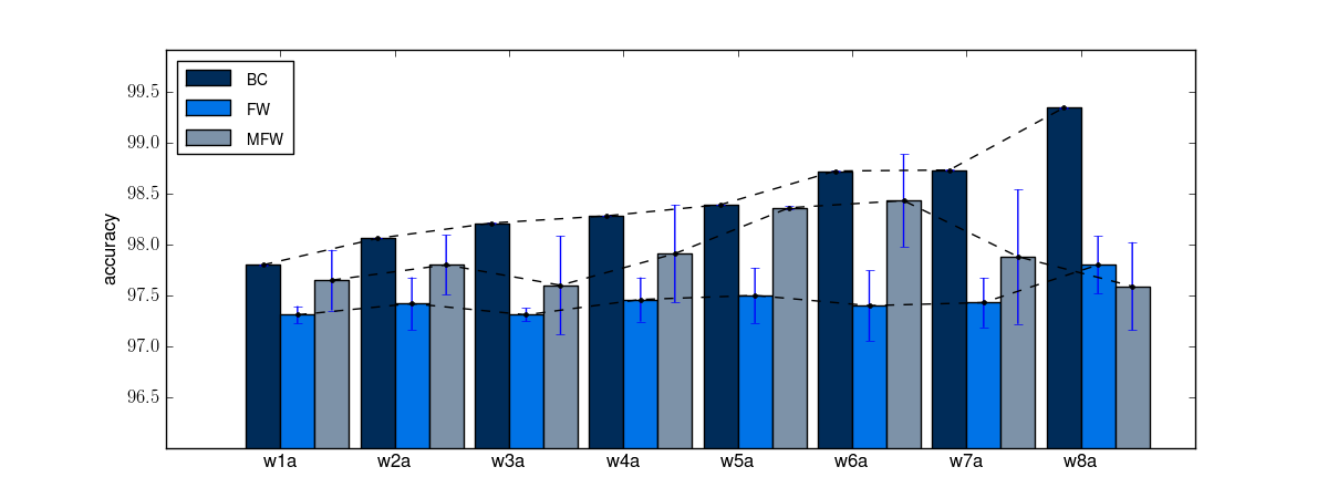
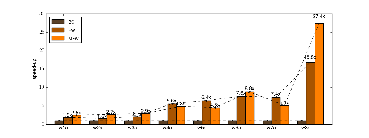
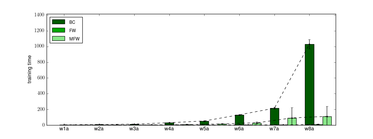
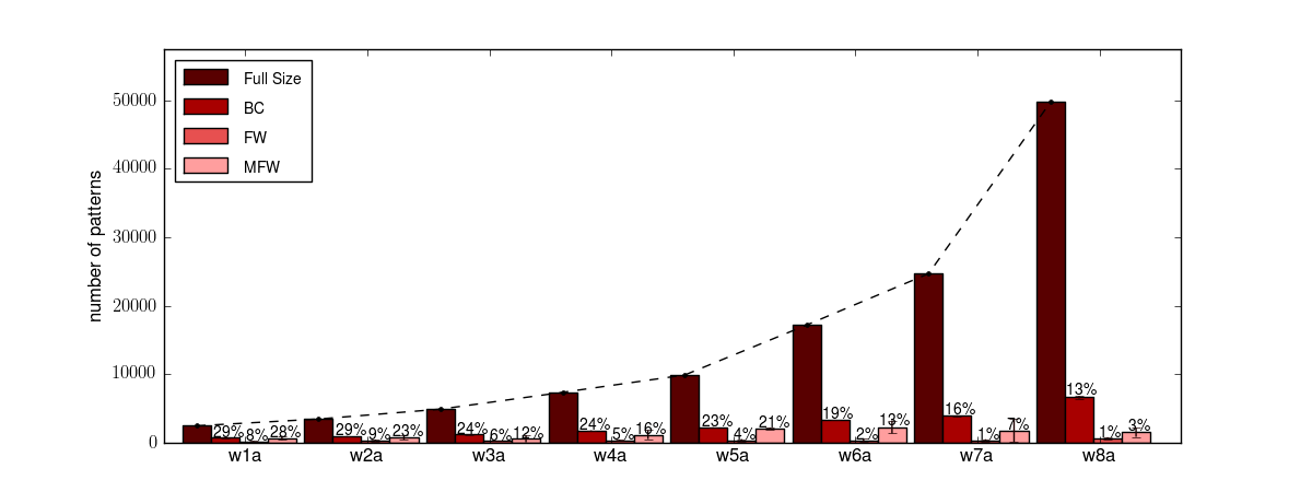
Figure 3: Comparison of accuracies (first row), speed-ups (second row), absolute running times (third row) and sizes of training sets and support vector sets (fourth row) in the Web datasets.

5.2.5 Computational Environment

The experiments were conducted on a personal computer with a 2.66GHz Quad Core CPU and 4 GB of RAM, running 64bit GNU/Linux (Ubuntu 10.10). The algorithms were implemented based on the (C++) source code available at [36].

5.3 Scalability Experiments on the Web Dataset Collection

In Fig. 3, we report some results concerning accuracies, training times, speed-ups and support vector set sizes obtained in the Web datasets. The series is monotonically increasing in the number of training patterns, which grows approximately as $m_{i}=1.4^{i}m_{0}$, $i=1,\ldots,8$, where $m_{0}$ is the number of training patterns in the first dataset [30].

The speed-up of the FW method with respect to CVMs is measured as $s=t_{0}/t_{1}$ where $t_{0}$ is the training time of the CVM algorithm and $t_{1}$ is the training time of the FW method, both measured in seconds. Similarly, the speed-up of the MFW method with respect to CVMs is measured as $s=t_{0}/t_{2}$ where $t_{2}$ is the training time of the MFW method.

As depicted in Fig. 3 the proposed methods are slightly less accurate than CVMs. The training time, in contrast, scales considerably better for our methods as the number of training patterns increases. The speed-ups are actually always greater than $1$, which shows that the FW and MFW methods indeed build classifiers faster than CVMs. More importantly, the speed-up is monotonically increasing, ranging from $12$ times faster up to $107$ times faster in the case of the FW algorithm and from $2$ times faster up to almost $10$ times faster in the case of the MFW method. This suggests that the improvements of the proposed method over CVMs becomes more and more significant as the size of the training set grows.

5.4 Scalability Experiments on the Adult Dataset Collection

Fig. 4 depicts accuracies and speed-ups obtained in the Adult datasets. Like the Web datasets, this collection was created with the purpose of analyzing the scalability of SVM methods and the number of training patterns grows approximately with the same rate [30]. The speed-up of the FW and MFW methods is computed as in the previous section.

Figure 4: Comparison of accuracies (first row), speed-ups (second row), absolute running times (third row) and sizes of training sets and support vector sets (fourth row) in the Adult datasets.

Results obtained in this experiment confirm that the proposed methods tend to be faster than CVMs as the dataset grows. CVMs are actually faster than FW just in two cases, corresponding to the smallest versions of the sequence. MFW however runs always faster than CVMs, reaching a speed-up of $15\times$ in the fifth version of the series. The speed-ups obtained by the FW method are in this experiment more moderate than in the Web collection. However, most of the time FW exhibits also better test accuracies than CVMs. Finally, the MFW algorithm is not only faster but also as accurate as CVMs on this classification problem.

5.5 Experiments on Single Datasets

Results of Figs. 5 and 6 correspond to accuracies and speed-ups obtained in the single datasets described in Tab. 1, that is, all of them but the Web and Adult series. Most of these problems have been already used to show the improvements of CVMs over other algorithms to train SVMs .

Results show that the proposed methods are faster than CVMs most of the time, sometimes at the price of a slightly lower accuracy. The speed-up achieved by FW and MFW becomes more significant as the size of the training set grows. FW in particular reaches peaks of $102\times$ in the second largest dataset (KDD99-10pc) and $25\times$ in the largest of the problems studied in this experiment (KDD99-Full). Finally, the results show that in the cases for which CVMs are faster, the advantage of this algorithm on FW and MFW tend to be very small, reaching its better speed-up against MFW in the USPS-Ext dataset, for which however FW exhibits a speed up of around $3\times$.

Dataset	CVM		FW		MFW
	Acc.	STD.	Acc.	STD.	Acc.	STD.
a1a	83.52	6.33E-003	83.52	7.53E-003	83.52	1.58E-003
a2a	83.55	1.15E-002	83.56	2.39E-002	83.56	9.19E-003
a3a	83.40	8.45E-003	83.39	4.17E-002	83.41	5.00E-003
a4a	84.06	1.59E-002	84.10	4.64E-002	84.07	1.15E-002
a5a	84.02	8.92E-003	84.03	2.93E-002	84.05	9.86E-003
a6a	84.28	3.51E-003	84.26	2.49E-002	84.25	1.86E-002
a7a	84.18	1.06E-002	84.23	4.41E-002	84.29	2.26E-002
w1a	97.80	2.81E-003	97.31	8.54E-002	97.65	2.97E-001
w2a	98.06	1.37E-003	97.42	2.58E-001	97.80	2.93E-001
w3a	98.21	1.67E-003	97.31	6.48E-002	97.60	4.83E-001
w4a	98.28	9.44E-004	97.46	2.17E-001	97.91	4.79E-001
w5a	98.39	2.01E-003	97.50	2.71E-001	98.36	1.76E-002
w6a	98.72	5.63E-003	97.40	3.45E-001	98.43	4.54E-001
w7a	98.73	5.29E-003	97.43	2.43E-001	97.88	6.60E-001
w8a	99.34	5.35E-003	97.80	2.82E-001	97.59	4.32E-001
Letter	97.48	2.19E-002	96.54	1.37E-001	97.35	1.50E-001
Pendigits	98.35	9.46E-002	97.68	9.39E-002	97.65	1.22E-001
USPS	95.63	3.73E-002	95.12	1.05E-001	95.47	8.34E-002
Reuters	97.10	4.11E-002	96.40	1.53E-001	95.60	6.13E-001
MNIST	98.46	3.14E-002	97.91	5.99E-002	98.36	4.05E-002
Protein	69.79	0.00E+00	69.73	0.00E+00	69.78	0.00E+00
Shuttle	99.67	1.51E-001	98.08	6.74E-001	97.82	1.54E+00
IJCNN	98.59	4.89E-002	95.71	7.95E-001	97.31	3.63E-001
USPS-Ext	99.50	1.26E-002	99.30	5.47E-002	99.57	2.76E-002
KDD10pc	99.87	2.06E-002	98.82	2.13E-001	99.10	2.86E-001
KDD-full	91.77	7.17E-002	91.53	1.14E+00	91.82	7.72E-002

Table 2: Test accuracy ($\%$) of the proposed algorithms and the baseline method CVM. Statistics correspond to the mean (Acc) and standard deviation (STD) obtained from $5$ repetitions of each experiment. For the Protein dataset, just $1$ repetition was carried out due to the significantly longer training times.

Dataset	CVM		FW		MFW
	Time	STD.	Time	STD.	Time	STD.
a1a	6.26	8.82E-02	12.5	6.99E-01	0.712	4.00E-03
a2a	16	1.82E-01	19.3	1.51E+00	1.46	1.41E-02
a3a	33.8	1.74E-01	26.8	1.44E+00	2.78	6.53E-02
a4a	89.1	2.67E-01	40.4	1.19E+00	6.37	1.08E-01
a5a	171	2.10E+00	56.1	1.94E+00	11.1	1.75E-01
a6a	590	2.62E+00	164	6.24E+00	45	1.15E+00
a7a	2060	2.79E+01	1420	5.86E+01	365	7.30E+00
w1a	3.59	3.62E-01	0.286	8.26E-02	1.67	7.62E-01
w2a	7.9	1.62E-01	0.658	3.32E-01	2.31	1.20E+00
w3a	12.8	1.11E+00	0.76	5.90E-02	2.27	2.25E+00
w4a	30.4	7.50E-01	1.26	5.01E-01	6.76	4.13E+00
w5a	52.7	6.39E-01	1.78	1.07E+00	15.8	1.44E+00
w6a	131	1.55E+00	2.67	2.36E+00	29.4	1.31E+01
w7a	215	1.17E+01	2.58	1.89E+00	91.4	1.31E+02
w8a	1030	6.05E+01	9.64	5.22E+00	111	1.27E+02
Letter	23.7	2.80E-01	13.3	2.05E-01	12.3	1.42E-01
Pendigits	0.554	3.26E-02	0.82	2.97E-02	0.658	2.23E-02
USPS	6.89	7.46E-02	7.58	1.42E-01	7.22	9.00E-02
Reuters	7.24	3.62E-01	2.17	3.87E-01	1.69	5.87E-01
MNIST	364	1.31E+01	301	8.56E+00	349	2.59E+00
Protein	247000	0.00E+00	11900	0.00E+00	2000	0.00E+00
Shuttle	1.41	3.41E-01	1.69	4.56E-01	0.176	2.73E-02
IJCNN	198	1.36E+01	40.5	2.27E+01	34.4	1.26E+01
USPS-Ext	84.4	2.02E+01	26.7	3.74E+00	161	1.49E+01
KDD10pc	42.3	3.58E+00	0.414	1.50E-02	1.22	1.24E+00
KDD-full	19.5	8.12E+00	0.764	2.42E-02	0.744	8.00E-03

Table 3: Running times (seconds) of the proposed algorithms and the baseline method CVM. Statistics correspond to the mean (Time) and standard deviation (STD) obtained from $5$ repetitions of each experiment. For the Protein dataset, just $1$ repetition was carried out due to the significantly longer training times.

For sake of readability we include in Tab. 2 and Tab. 3 a summary of the test accuracy and running times used to build the Figs. 3 to 6.

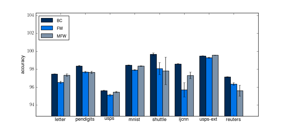
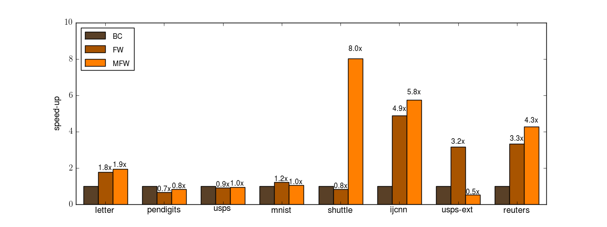
Figure 5: Comparison of accuracies (first row) and speed-ups (second row) obtained in some of the single datasets of Tab. 1

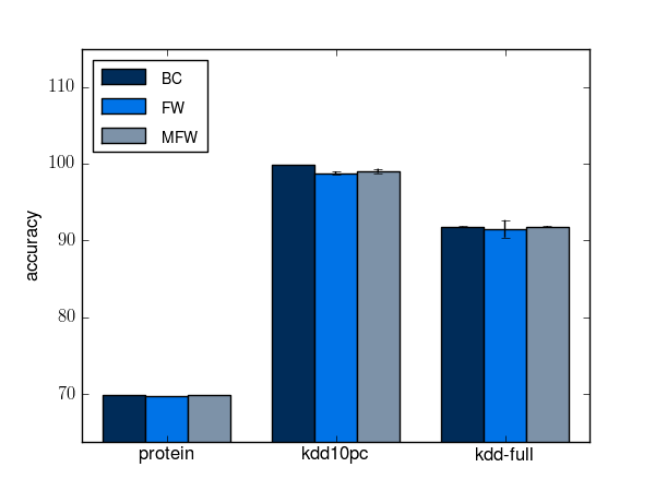
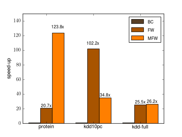
Figure 6: Comparison of accuracies (first column) and speed-ups (second column) obtained in some of the single datasets of Tab. 1

5.6 Statistical Tests

This paragraph is devoted to verify the statistical significance of the results obtained above. To this end we adopt the guidelines suggested in [7], that is, we first conduct a multiple test to determine whether the hypothesis that all the algorithms perform equally can be rejected or not. Then, we conduct separate binary tests to compare the performances of each algorithm against each other. For the binary tests we adopt the Wilcoxon Signed-Ranks Test method. For the multiple test we use the non-parametric Friedman Test. In [7], Demsar recommends these tests as safe alternatives to the classical parametric t-tests to compare classifiers over multiple datasets.

The main hypothesis of this paper is that our algorithms are faster than CVM. We have also observed than they are slightly less accurate. Therefore, our design for the binary tests between our algorithms and CVM is that of Tab. 7. As regards the comparison of the proposed methods, there is no an apparent advantage in terms of running time of one against the other. MFW seems however more accurate than FW. We thus conduct a two-tailed test for the running times but adopt a one-tailed test for testing accuracy.

	FW vs. CVM
Time	$H_{0}:\,\mbox{FW and CVM are equally fast}$
	$H_{1}:\,\mbox{FW is faster than CVM}\,$
Accuracy	$H_{0}:\,\mbox{FW and CVM are equally accurate}$
	$H_{1}:\,\mbox{CVM is more accurate than FW}\,$

	MFW vs. CVM
Time	$H_{0}:\,\mbox{MFW and CVM are equally fast}$
	$H_{1}:\,\mbox{MFW is faster than CVM}\,$
Accuracy	$H_{0}:\,\mbox{MFW and CVM are equally accurate}$
	$H_{1}:\,\mbox{CVM is more accurate than MFW}\,$

	FW vs. MFW
Time	$H_{0}:\,\mbox{FW and MFW are equally fast}$
	$H_{1}:\,\mbox{Running times of MFW and FW are different}\,$
Accuracy	$H_{0}:\,\mbox{FW and MFW are equally accurate}\,$
	$H_{1}:\,\mbox{FW is less accurate than MFW}\,$

Table 4: Null and alternative hypotheses for the binary statistical tests.

In Tab. 5 we report the values of the tests statistics calculated on the 26 datasets used in this paper. The critical values for rejection of the null hypothesis under a given significance level can be obtained in several books [26]. Here, in Tab. 6, we report the p-values corresponding to each test.

	W statistic			F statistic
	FW vs. CVM	MFW vs. CVM	FW vs. MFW	FW,MFW,CVM
Time	17	20	159	14.858
Accuracy	19	48.5	63.5	11.879

Table 5: Values of the W and F statistics for Wilcoxon Signed-Ranks Tests and Friedman Tests respectively.

	Binary Tests			Multiple Tests
	FW vs. CVM	MFW vs. CVM	FW vs. MFW	FW,MFW,CVM
Time	$3.085e-06$	$5.528e-06$	$0.6893$	$1.72e-05$
Accuracy	$4.977e-06$	$3.21e-04$	$1.23e-03$	$1.20e-04$

Table 6: P-values corresponding to the statistical tests.

Note that in all but one case (binary test FW vs. MFW about running time) the p-values are lower than $0.01$. Therefore, for most commonly used significance levels ($0.01$, $0.05$, $0.1$, or lower) we conclude that there are significant differences in terms of time and accuracy among the algorithms. Table 7 summarizes the conclusions from the binary tests. Note that the main hypothesis of this paper is confirmed. Most of the time our algorithms run faster and are less accurate. In the previous sections we have seen however that the loss in accuracy is usually lower than $1\%$, while the running time can be order of magnitudes better. As regards the comparison of the proposed algorithms FW and MFW, we cannot conclude that the difference in training time is statistically significant. However, we conclude that MFW is more accurate than FW. This last observation stresses the relevance of this work as an extension of the results presented in [10].

	FW vs. CVM
Time	$H_{0}$ rejected, so $H_{1}:\,\mbox{FW is faster than CVM}\,$
Accuracy	$H_{0}$ rejected, so $H_{1}:\,\mbox{CVM is more accurate than FW}\,$

	MFW vs. CVM
Time	$H_{0}$ rejected, so $H_{1}:\,\mbox{MFW is faster than CVM}\,$
Accuracy	$H_{0}$ rejected, so $H_{1}:\,\mbox{CVM is more accurate than MFW}\,$

	FW vs. MFW
Time	We cannot reject $H_{0}:\,\mbox{FW and MFW are equally fast}$
Accuracy	$H_{0}$ rejected, so $H_{1}:\,\mbox{FW is less accurate than MFW}\,$

Table 7: Conclusions from the binary statistical tests for significance levels $0.01$, $0.05$, $0.1$.

5.7 Experiments on the parameter $C$

Previous experiments have shown that parameter $C$ used by SVMs to handle noisy patterns can have a significant impact on the training time required to build the classifier [10]. We hence conduct experiments on some datasets to study this effect in more detail.

Figs. 7 and 8 show the training times and accuracies obtained in the Shuttle, KDD99-10pc, Pendigits and Reuters datasets when changing the value of $C$. Results confirm the general effect of this parameter on the training time: as $C$ grows all the algorithms become faster. However the training times of the proposed methods are most of time significantly lower than those of CVMs, independently of the value of parameter $C$ used by the SVM.

Figure 7: Test accuracies (first row) and training times (second row) obtained while changing the value of $C$ in the Shuttle and KDD99-10pc datasets.

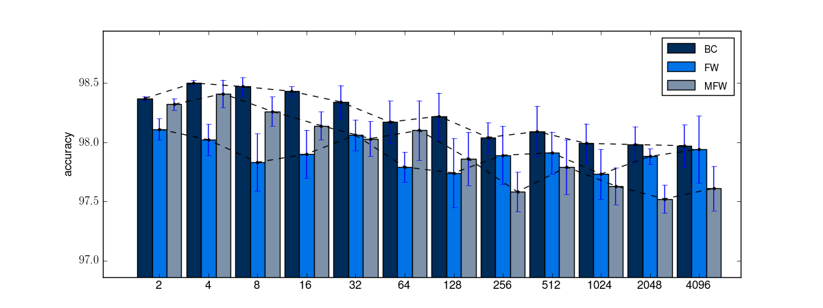
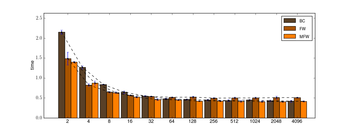
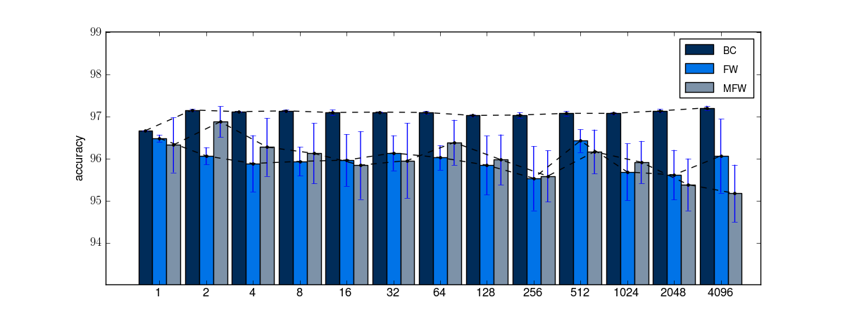
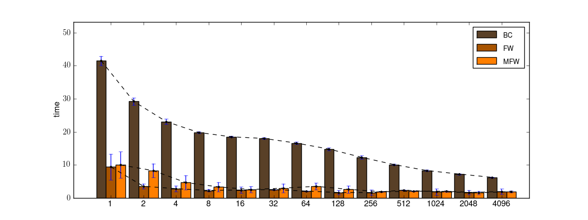
Figure 8: Test accuracies (first row) and training times (second row) obtained while changing the value of $C$ in the Pendigits and Reuters datasets.

5.8 Experiments with Non-Normalized Kernels

Solving a classification problem using SVMs requires to select a kernel function. Since the optimal kernel for a given application cannot be specified a priori, the capability of a training method to work with any (or the widest possible) family of kernels is an important feature.

In order to show that the proposed methods can obtain effective models even if the kernel does not satisfy the conditions required by CVMs, we conduct experiments using the homogeneous second order polynomial kernel $k(\mathbf{x}_{i},\mathbf{x}_{j})=(\gamma\mathbf{x}_{i}^{T}\mathbf{x}_{j})^{2}$. Here, parameter $\gamma$ is estimated as the inverse of the average squared distance among training patterns. Parameter $C$ is determined as usual by using a validation grid search on the values $2^{0},2^{1},\ldots,2^{12}$. The test set is never used to determine SVMs meta-parameters.

Note however that the purpose of this section is not to determine an optimal choice of the kernel function on the considered problems. The results presented below are merely indicative of the capability of the FW and MFW methods to handle a wide family of kernels, thus allowing for a greater flexibility in building a classifier.

Tab. 8 summarizes the results obtained in some of the datasets used in this section. We can see that both test accuracies and training times are comparable to those obtained using the gaussian kernel. It should be noted that the CVM algorithm cannot be used to train an SVM using the kernel selected for this experiment and thus we only incorporate the FW and MFW methods in the table. These results demonstrate the capability of our methods to be used with kernels other than those satisfying the normalization condition imposed by CVMs.

Dataset	Algorithm	Accuracy	STD-Accuracy	Time(s)	STD-Time
Shuttle	FW	96.58	9.44E-01	6.32E+01	3.69E+01
Shuttle	MFW	95.86	9.33E-01	8.52E+01	1.29E+02
Reuters	FW	95.80	3.00E-01	2.89E+00	3.23E-01
Reuters	MFW	95.90	1.98E-01	2.39E+00	1.52E-01
Web w1a	FW	97.22	1.08E-01	7.60E-02	3.50E-02
Web w1a	MFW	97.49	1.47E-01	2.52E-01	1.34E-01
Web w2a	FW	97.33	1.65E-01	1.42E-01	1.11E-01
Web w2a	MFW	97.09	1.93E-01	8.40E-02	6.53E-02
Web w3a	FW	97.32	1.68E-01	2.64E-01	1.33E-01
Web w3a	MFW	97.22	1.22E-01	3.18E-01	3.19E-01
Web w4a	FW	97.16	1.43E-01	3.76E-01	3.22E-01
Web w4a	MFW	97.25	1.49E-01	3.74E-01	3.65E-01
Web w5a	FW	97.08	7.37E-02	1.54E-01	2.14E-01
Web w5a	MFW	97.11	1.12E-01	2.78E-01	3.20E-01
Web w6a	FW	97.28	2.37E-01	2.96E-01	2.37E-01
Web w6a	MFW	97.18	1.31E-01	5.02E-01	4.11E-01
Web w7a	FW	97.23	6.22E-02	3.88E-01	2.81E-01
Web w7a	MFW	97.23	1.51E-01	2.10E-01	1.35E-01
Web w8a	FW	97.06	1.10E-01	2.76E-01	2.32E-01
Web w8a	MFW	97.24	2.91E-01	3.38E-01	3.32E-01

Table 8: Accuracies and training times obtained with a polynomial kernel. Statistics correspond to the mean and standard deviation obtained from $5$ repetitions of each experiment.

5.9 Discussion

We now comment in more detail the results presented above. First of all we note that, most of the time, the proposed algorithms appear very competitive against CVM, with a tendency to favor training speed in large datasets, sometimes at the expense of a little accuracy. CVMs appear faster than FW just in three problems among the single datasets studied in Subsection 5.5: Pendigits, USPS and Shuttle. It should be noted however that the Pendigits and USPS datasets correspond to multi-category problems and are approached using a decomposition method based on solving several binary subproblems. Now, as shown in Tab. 1, the greatest binary subproblem for these datasets, is smaller than all the problems of the Web collection and all but one of the Adult collection. When each subproblem is very small, SMO iterations are quite cheap, and the overall cost of running the BC procedure is reasonably low. In these cases, training with a CVM (or even with a traditional SMO-based SVM) possibly constitutes a convenient choice. The advantage of FW-based methods lies instead in their capability to effectively handle larger problems, as results on the Web and Adult collections show.

All the methods offer very similar testing performances on all the character recognition problems (Letter, Pendigits, MNIST, USPS-Scaled and USPS-Ext). On datasets IJCNN and Reuters, CVM offers more accurate classifiers but employs a larger running time compared to FW and MFW. The same can be said about the KDD99-10pc problem, but in this case the speed-up offered by FW and MFW is considerably larger, up to two orders of magnitude. The Shuttle dataset returns mixed results, which are probably due to the high lack of homogeneity in the size of the subproblems solved in the OVO decomposition approach. Finally, the two FW methods are clearly advantageous on Protein and KDD99-Full datasets, where they offer the same accuracy of CVMs along with a considerably improved running time.

The results on the Web and Adult datasets are of particular interest and deserve further comment. They consist of a series of datasets of increasing size, and from their study we expect to gain an understanding of the performance of the algorithm as $m$ gradually increases. In fact, as documented in [30] and [25] these datasets have been commonly used to compare the scalability of SVM algorithms. In this regard, our results appear very encouraging. Not only do both FW algorithms outperform CVM in every instance of the Web collection with respect to CPU time, but the observed speedup increases monotonically as the dataset size increases, reaching a peak of two orders of magnitude for the FW method. Both algorithms also outperforms running times of CVM on all but two datasets of the Adult collection, with very similar testing accuracies.

The clear advantage of the MFW method with respect to both FW and CVM in the Adult series can be probably explained by the considerable size of the support vector set, which roughly amounts to a $60\%$ of the full dataset, for all the methods. It is evident that, if $\mathcal{C}_{k}$ becomes large, SMO iterations become quite expensive, slowing down the CVM procedure. As regards the advantage of MFW over FW, we interpret the results as follows. At the beginning of the training process, the algorithms start with a small approximating ball, and progressively expand it by including new examples. Intuitively, in the first iterations both methods tend to include a large number of points in order to increase the radius of the ball (and thus the objective value). Some of these examples do not belong to the optimal support vector set and the algorithms will try to remove them from the model once they approach the solution. When the support vector set is large, as in this case, the number of these spurious examples can be quite large, hampering the progress towards the optimum. Now, FW is not endowed with the possibility of explicitly removing points from the current coreset approximation, implying that the weights of useless patterns vanish only in the limit. That is, a large number of iterations may be taken before they drop below the tolerance under which they are numerically considered zeros. MFW, in contrast, possesses the ability to remove undesired points directly, and thus enjoys a considerable advantage when the number of such examples is not small.

6 Conclusions and Perspectives

In this paper we have described the application of $\epsilon$–coreset based methods from computational geometry to the task of efficiently training an SVM, an idea first proposed in [37]. We have introduced two algorithms falling in this category, both based on the Frank-Wolfe optimization scheme. These methods use analytical formulas to learn the classifier from the training set and thus do not require the solution of nested optimization subproblems. Compared with the results we presented in [10], we have explored a variant of the algorithm which compares favorably in terms of testing accuracy and achieves training times similar to our original version.

The large set of experiments we report in this paper confirms and considerably expands the conclusions reached in [10]. As long as a minor loss in accuracy is acceptable, both Frank-Wolfe based methods are able to build SVM classifiers in a considerably smaller time compared to CVMs, which in turn have been proven in [37] to be faster than most traditional SVM software. These conclusions were statistically assessed using non-parametric tests. A second contribution of this work has been to present preliminary evidence about the capability to handle a wider family of kernels than CVMs, thus allowing for a greater flexibility in building a classifier. Further variations of this procedure will be explored in a future work, including learning tasks other than classification.

References

- [1] S. Asharaf, M. Murty, and S. Shevade. Multiclass core vector machine. In Proceedings of the ICML’07, pages 41–48. ACM, 2007.
- [2] M. Bădoiu and K. Clarkson. Smaller core-sets for balls. In Proceedings of the SODA’03, pages 801–802. SIAM, 2003.
- [3] C.-C. Chang and C.-J. Lin. LIBSVM: a library for support vector machines, 2010.
- [4] K. Clarkson. Coresets, sparse greedy approximation, and the Frank-Wolfe algorithm. In Proceedings of SODA’08, pages 922–931. SIAM, 2008.
- [5] C. Cortes and V. Vapnik. Support-vector networks. Machine Learning, 20:273–297, 1995.
- [6] K. Crammer and Y. Singer. On the algorithmic implementation of multiclass kernel-based vector machines. Journal of Machine Learning Research, 2:265–292, 2001.
- [7] J. Demsar. Statistical comparison of classifiers over multiple data sets. Journal of Machine Learning Research, 7:1–30, 2006.
- [8] R.-E. Fan, P.-H. Chen, and C.-J. Lin. Working set selection using second order information for training support vector machines. Journal of Machine Learning Research, 6:1889–1918, 2005.
- [9] S. Fine and K. Scheinberg. Efficient SVM training using low-rank kernel representations. Journal of Machine Learning Research, 2:243–264, 2002.
- [10] E. Frandi, M. G. Gasparo, S. Lodi, R. Ñanculef, and C. Sartori. A new algorithm for training SVMs using approximate minimal enclosing balls. In Proceedings of the 15th Iberoamerican Congress on Pattern Recognition, Lecture Notes in Computer Science, pages 87–95. Springer, 2010.
- [11] M. Frank and P. Wolfe. An algorithm for quadratic programming. Naval Research Logistics Quarterly, 1:95–110, 1956.
- [12] G. Fung and O. L. Mangasarian. Finite newton method for lagrangian support vector machine classification. Neurocomputing, 55(1-2):39–55, 2003.
- [13] J. Guélat and P. Marcotte. Some comments on Wolfe’s “away step”. Mathematical Programming, 35:110–119, 1986.
- [14] T. Hastie, R. Tibshirani, and J. Friedman. The elements of statistical learning: data mining, inference, and prediction: with 200 full-color illustrations. New York: Springer-Verlag, 2001.
- [15] S. Hettich and S. Bay. The UCI KDD Archive. http://kdd.ics.uci.edu, 2010.
- [16] T. Hofmann, B. Schölkopf, and A. J. Smola. Kernel methods in machine learning. Annals of Statistics, 36(3):1171–1220, 2008.
- [17] C. Hsu and C. Lin. A comparison of methods for multiclass support vector machines. IEEE Transactions on Neural Networks, 13(2):415–425, 2002.
- [18] T. Joachims. Making large-scale support vector machine learning practical. In Advances in kernel methods: support vector learning, pages 169–184. MIT Press, 1999.
- [19] U. Kressel. Pairwise classification and support vector machines. In Advances in kernel methods: support vector learning, pages 255–268. MIT Press, Cambridge, MA, USA, 1999.
- [20] K. Kumar, C. Bhattacharya, and R. Hariharan. A randomized algorithm for large scale support vector learning. In Advances in Neural Information Processing Systems 20, pages 793–800. MIT Press, 2008.
- [21] P. Kumar, J. Mitchell, and E. A. Yildirim. Approximate minimum enclosing balls in high dimensions using core-sets. Journal of Experimental Algorithmics, 8:1.1, 2003.
- [22] Y. Lee and S. Huang. Reduced support vector machines: A statistical theory. IEEE Transactions on Neural Networks, 18(1):1–13, 2007.
- [23] Y. Lee, Y. Li, and G. Wahba. Multicategory support vector machines: Theory and application to the classification of microarray data and satellite radiance data. Journal of the American Statistical Association, 99(465):67–81, 2004.
- [24] Y. Lee and O. L. Mangasarian. RSVM: reduced support vector machines. In Proceedings of the first SIAM International Conference on Data Mining, pages 325–361. SIAM, 2001.
- [25] O. L. Mangasarian and D. R. Musicant. Successive overrelaxation for support vector machines. IEEE Transactions on Neural Networks, 10:1032–1037, 1999.
- [26] W. Mendenhall. Introduction to probability and statistics (13th Ed.). Duxbury Press, 2009.
- [27] D. Michie, D. Spiegelhalter, and C. Taylor. Machine Learning, Neural and Statistical classification. Prentice Hall, Englewood Cliffs, NJ, 1994.
- [28] R. Ñanculef, C. Concha, H. Allende, and C. Moraga. AD-SVMs: A light extension of SVMs for multicategory classification. International Journal of Hybrid Intelligent Systems (to appear), 2009.
- [29] D. Pavlov, J. Mao, and B. Dom. An improved training algorithm for support vector machines. In Proceedings of the 15th International Conference on Pattern Recognition, volume 2, pages 2219–2222. IEEE, 2000.
- [30] J. Platt. Fast training of support vector machines using sequential minimal optimization. In Advances in kernel methods: support vector learning, pages 185–208. MIT Press, 1999.
- [31] R Core Team. R: A Language and Environment for Statistical Computing. R Foundation for Statistical Computing, Vienna, Austria, 2012. ISBN 3-900051-07-0.
- [32] K. Scheinberg. An efficient implementation of an active set method for SVMs. Journal of Machine Learning Research, 7:2237–2257, 2006.
- [33] B. Schölkopf and A. J. Smola. Learning with Kernels: Support Vector Machines, Regularization, Optimization, and Beyond. MIT Press, 2001.
- [34] B. Schölkopf and A. J. Smola. Sparse greedy matrix approximation for machine learning. In Proceedings of the 17th International Conference on Machine Learning, pages 911–918, 2001.
- [35] A. J. Smola and P. Bartlett, editors. Advances in Large Margin Classifiers. MIT Press, Cambridge, 2000.
- [36] I. Tsang, A. Kocsor, and J. Kwok. LibCVM Toolkit, 2009.
- [37] I. Tsang, J. Kwok, and P.-M. Cheung. Core vector machines: Fast SVM training on very large data sets. Journal of Machine Learning Research, 6:363–392, 2005.
- [38] I. Tsang, J. Kwok, and J. Zurada. Generalized core vector machines. IEEE Transactions on Neural Networks, 17(5):1126–1140, 2006.
- [39] V. Vapnik. The nature of statistical learning theory. Springer-Verlag, 1995.
- [40] P. Wolfe. Convergence theory in nonlinear programming. In J. Abadie, editor, Integer and Nonlinear Programming, pages 1–36. North-Holland, Amsterdam, 1970.
- [41] E. A. Yildirim. Two algorithms for the minimum enclosing ball problem. SIAM Journal on Optimization, 19(3):1368–1391, 2008.