Resource dependent branching processes
and the envelope of societies

Abstract

Since its early beginnings, mankind has put to test many different society forms, and this fact raises a complex of interesting questions. The objective of this paper is to present a general population model which takes essential features of any society into account and which gives interesting answers on the basis of only two natural hypotheses. One is that societies want to survive, the second, that individuals in a society would, in general, like to increase their standard of living. We start by presenting a mathematical model, which may be seen as a particular type of a controlled branching process. All conditions of the model are justified and interpreted. After several preliminary results about societies in general we can show that two society forms should attract particular attention, both from a qualitative and a quantitative point of view. These are the so-called weakest-first society and the strongest-first society. In particular we prove then that these two societies stand out since they form an envelope of all possible societies in a sense we will make precise. This result (the envelopment theorem) is seen as significant because it is paralleled with precise survival criteria for the enveloping societies. Moreover, given that one of the “limiting” societies can be seen as an extreme form of communism, and the other one as being close to an extreme version of capitalism, we conclude that, remarkably, humanity is close to having already tested the limits.

and

1 Introduction

What is the goal of any society? Are there natural boundaries for societies mankind would not or cannot exceed? And if so, can we quantify the critical parameters characterizing these boundaries? Certain aspects of these questions are equally interesting for animal societies; in fact, throughout this paper we shall always speak of “individuals” to make clear that, although the motivation stems from thinking about man, we keep general populations in mind.

The first question is partially philosophical, and we only treat it in as much as it concerns the subsequent questions. Here we shall provide a mathematical answer obtained from a model we propose as a global mathematical model for societies. This model is built on branching processes and submitted to two natural hypotheses. Still rudimentary, the model is broad enough to allow for essential features of life within any society: reproduction of individuals, the desire to have a future, heritage and production of resources, consumption of resources, policies to distribute resources among individuals, and, as a tool of interaction, the right of emigration. We look at different sub-models of the model, characterizing different societies. These are defined by the type of control they exercise through different policies to distribute resources among their individuals.

1.1 Objectives of societies

Any society is likely to advertise certain keywords in its program or mission statement, such as justice, liberty, equal opportunity, etc. We all agree that these issues are likely to be important. However, there may be as many different interpretations of them as there are individuals in a population. Hence, within a whole population they can hardly serve as real guidelines for the choice of a specific society form. We conclude that any reasonable approach must be more focused.

The philosophy of our approach to answering questions about the choice of a society is therefore to focus on factors which are seen as dominant, namely those which come out of two natural and seemingly inoffensive hypotheses:

Hypothesis 1.

Individuals want to survive and to see a future for their descendants.

Hypothesis 2.

Individuals prefer, in general, a higher standard of living to a lower one.

Since these hypotheses may not be compatible with each other, we define Hypothesis 1 to have a higher priority than Hypothesis 2.

Other hypotheses may be implicit. For instance, the desire to have security is implicit in Hypothesis 2. If the standard of living is sufficiently high, the society can afford a qualified police force or a strong army.

To deal with these hypotheses in an adequate way, the problem is to find a suitable model. This requires two important conditions. First, the model should allow for all mentioned features which are seen as essential for the development of a human society and also for a clear interaction of individuals within the society. Second, it should be sufficiently tractable to allow for quantifiable conclusions.

1.2 History of results

The first-named author has been thinking about ways to model societies for many years. He had given a first talk on resource dependent branching processes in 1983, a second around 1995 and a third in 2001. Although the publications Bruss (1984) and Bruss and Robertson (1991) were motivated by thinking about such processes, this is the very first paper devoted to this subject.

In the beginning, only preliminary results about necessary conditions for survival were obtained, and only for an elementary model. These results were based on earlier work on branching processes with random absorbing processes, on $\varphi$-branching processes, and on different forms of the Borel–Cantelli lemma.

In a second step, several models were tested until the model presented here took its approximate shape. When seeing, in a different context, the article by Coffman, Flatto and Weber (1987), the results were sharpened to our needs in Bruss and Robertson (1991). These opened the way to quantifiable conclusions for the chosen model and thus to survival criteria for several special societies.

In a third step it became visible that, in any reasonable model, two societies deserved special attention. These are what we call the strongest-first society (s.f.-society), and the weakest-first society (w.f.-society). A survival criterion for the w.f.-society was proved; survival criteria for the s.f.-society were tested, and the idea of a theorem of envelopment began to emerge.

The fourth step (with the co-author) brought a broad definition of general policies as well as a proof of a survival criterion for the s.f.-process. It also led to the precise formulation and proof of the envelopment theorem for societies. This theorem says (in both a conditional and an unconditional form) that all societies are bound to live in the long run between the s.f.-society and the w.f.-society. Combined with all earlier findings, we think this is a fundamental result.

1.3 Related work

Our model is an asexual controlled branching process (BP), where controlled should be understood in an interacting sense. The general control is governed by functions of sums of dependent variables, and self-imposed. This strong dependence property excludes the generating function machinery, of course. Moreover, although still rudimentary, the model seems no longer to profit from martingale arguments.

Early work on controlled BPs confined interest to control through bounds imposed on the growth of Galton–Watson-type processes. Sevast’janov and Zubkov (1974), Schuh (1976) and others modified the number of individuals which are allowed to reproduce in each generation by corresponding deterministic functions. Bruss (1978) considered a Galton–Watson process (GWP) with a nonspecified absorbing process for which only the expected influence is known.

Yanev (1976) studied so-called $\phi$-branching processes where the growth of the GWP reproduction is controlled by random numbers of offspring which are allowed to reproduce. A more general model for random control functions was studied in Bruss (1980), and again in more generality, by González, Molina and Del Puerto (2002). The same authors also examined $L_{2}$-convergence for such processes; see González, Molina and del Puerto (2005).

Population-size dependence is another interesting access to control in BP models. These were studied by Klebaner (1985) and Cohn and Klebaner (1986). Xu and Mannor (2012) proposed a special class of controlled BPs involving a different notion of “resources.” Motivated by applications in marketing, the objective is to control independent subpopulations (multi-type model) in such a way that they grow as quickly as possible. Relative frequencies of types were studied in Yakovlev and Yanev (2009).

The model presented in this paper is neither a BP with varying environment [see, e.g., Cohn (1996)] nor a BP with random environment. See Jagers (1975) for a clear analysis of the connection between these two types, and, for example, Haccou, Jagers and Vatutin (2007) for newer developments. Our model is neither a multi-type BP nor a pure population size-dependent model. It is a Markov process, as we shall see, but no phase-type Markov model or decomposable BP [see Hautphenne (2012)] can play the control we have in mind.

Hence, our model does not fit these or similar models studied in the literature. Nevertheless, related work is sincerely acknowledged. It has helped, over the years, to get a feeling of what result one can, or cannot, possibly hope for.

2 The model

We consider a population, beginning at time $0$ with a fixed number of individuals, which reproduce at distinct times $n\in\mathbb{N}_{0}$. The time interval $[n,n+1)$ is called the $n$th generation. Individuals consume resources and create new resources for their descendants. Only those descendants whose resource claims will be met by society will stay within the population until the next reproduction time; the others are supposed to emigrate (or die) before reproduction. We first define all the components of the model.

2.1 Reproduction

Individuals are supposed to reproduce independently of each other. The model supposes that reproduction is asexual. The number of descendants of each individual is modeled according to a common probability law $(p_{j})_{j\in\mathbb{N}}$, where $p_{j}$ denotes the probability that a given individual will have exactly $j$ offspring. To avoid trivial cases, we suppose $p_{0}>0$ and $p_{j}>0$ for at least some $j>1$. Let $D_{n}^{k}$ denote the number of descendants of the $k$th individual in the $n$th generation. Hence $\mathrm{P}[D_{n}^{k}=j]=p_{j}$, for all $n\in\mathbb{N},k\in\mathbb{N}_{0}$ and all $j\in\mathbb{N}$. The infinite double-array $(D_{n}^{k})_{n\in\mathbb{N},k\in\mathbb{N}_{0}}$, named reproduction matrix, thus consists of independent identically distributed (i.i.d.) integer-valued nonnegative random variables with mean $m:=\mathrm{E}(D_{n}^{k})<\infty$.

2.2 Resources and resource space

Human beings need food; they need resources. They also reproduce, and thus they need resources for their descendants. Hence they must save resources and create resources for future generations.

In our model, individuals inherit resources from preceding generations, consume resources and create new resources. The resources an individual can use during his lifetime determines his standard of living. The society decides in what way resources are distributed among the individuals, or expressed differently, it is the acceptance of policies to distribute resources that defines a society. The inherited resources, plus the newly created ones, are, after deduction of consumption, considered to be the individual’s contribution to the common resources of the society, called the resource space.

We do not distinguish between heritage, new production and nonconsumption of resources and summarize heritage plus production minus consumption as creation of resources. Resource creations of individuals are modeled as i.i.d. real-valued nonnegative random variables $R_{n}^{k}$, $n\in\mathbb{N},k\in\mathbb{N}_{0}$, and the infinite double array $(R_{n}^{k})_{n\in\mathbb{N},k\in\mathbb{N}_{0}}$ will be called resource creation matrix. We suppose that $r:=\mathrm{E}(R_{n}^{k})<\infty$.

2.3 Objective of survival

The population’s desire to survive is understood as the objective to have for the society as a whole a positive probability of surviving forever. If certain rules to distribute resources allow for a positive probability of survival, and if other rules do not achieve this, then the objective to survive takes priority, and the rules are changed accordingly. It suffices to see changes as an omnipresent option and to think of the rules defining the society, even if they had been changed many times before, as being fixed from today onward for the whole future. (This “fixed future-instant control” assumption has the advantage that society need not be expected to have long-term prophetical abilities.)

2.4 Resource claims within a society

The model interprets for each descendant, the individual claim of resources as the outcome of two random components. One is the descendant’s desire to have a certain amount of resources, and the other is what the descendant, with its own power of conviction, will be able to defend among its competitors within the society.

These random claims of individuals are modeled as i.i.d. real-valued nonnegative random variables governed by a known continuous distribution function $F$. If there are $t_{n}$ descendants in the $n$th generation they generate a string of claims $(X_{n}^{1},X_{n}^{2},\ldots,X_{n}^{t_{n}})$. The infinite double array $(X_{n}^{k})_{n\in\mathbb{N},k\in\mathbb{N}_{0}}$, is called claim matrix. We have $F(x)=\mathrm{P}[X_{j}^{k}\leq x]$ and suppose $\mu:=\break\mathrm{E}(X)<\infty$.

2.5 Interaction of individuals and society

Each individual is supposed to have the right to emigrate, and the control instrument is the right to exercise the option of emigration. To fix the rules, we suppose that an individual emigrates if and only if his individual resource claim is not completely satisfied by the society; otherwise he remains a member of the population until the end of the generation. Emigration is supposed to happen before an individual produces offspring. Hence each individual resource assignment (seen as the individual standard of living offered by the society) is felt by an individual as being either sufficient, implying “stay,” or else insufficient, implying “leave.”

Typically, the total resource space created by a generation is insufficient to satisfy all the resource claims of the offspring. We define a policy as a function which determines then a priority order among offspring, that is, a rule to distribute the resources created by the current generation among the next generation.

2.5.1 Examples

To keep examples simple we use here positive integers for claims and available resources; this is not required in reality, of course. Any random claim expresses the number of units of resources the individual requires. Assume, for instance, that, in a given generation, the number of individuals is $10$, and that the current resource space is $100$. Suppose further that the individuals write down their claims on a list in some order, as, for instance, in chronological order of arrival of claims, and that the string of claims reads

$$11,7,15,19,11,18,10,22,17,19.$$

The “first-come-first-served” society would grant the first seven claims(adding up to $91$), and the last three applicants would then have to emigrate. The $9$ remaining units may be divided among the seven or put back into the common resources. (Details on this level will not matter for our results.) A society that distributes resources in f.c.f.s.-order may not have much appeal, as one may argue. However there are certainly more foolish policies, as, for example, the “coin-flipping policy” which chooses the priority order at random. Any procedure to select a priority of claims is considered a policy.

In the sequel, two particular policies will attract our special interest: the first one, called the weakest-first society, satisfies the smallest claims first and would thus retain, in the example above, the claims $7,10,11,11,15,17,18$, while the other, called the strongest-first society, satisfies the largest claims first and would thus retain the claims $22,19,19,18,17$.

2.6 Resource dependent branching processes

We now give a precise definition of the type of population processes we consider in this paper. Two definitions are needed. Let $((D^{k}_{n})_{n\in\mathbb{N},k\in\mathbb{N}_{0}},(X^{k}_{n})_{n\in\mathbb{N},k\in\mathbb{N}_{0}},(R^{k}_{n})_{n\in\mathbb{N},k\in\mathbb{N}_{0}})$ be a triplet of independent double arrays of i.i.d. random variables defined on a probability space $(\Omega,\mathcal{F},\mathrm{P})$. As before, the variables $D_{n}^{k}$, $X_{n}^{k}$ and $R_{n}^{k}$ ($k\in\mathbb{N}_{0}$) represent the number of offspring, the resource claims and the production of resources (resp.) of each individual (labeled by $k$) in generation $n$. We always assume that these variables satisfy the natural regularity conditions given below; see Section 2.7. Let

$$D_{n}(k):=\sum_{j=1}^{k}D_{n}^{j}\quad\mbox{and}\quad R_{n}(k):=\sum_{j=1}^{k}R_{n}^{j}$$ (1)

denote the total number of offspring and the total resources created by generation $n$, respectively, given that generation $n$ counts $k$ individuals. The i.i.d. assumptions for random variables within the same double array allow us to use the shorter notation $D(k)=D_{n}(k)$ and $R(k)=R_{n}(k)$ whenever we limit our interest to their distributional prescriptions. Conversely, this is understood throughout the paper whenever we use this simplified notation.

We first need a precise definition of a policy:

Definition 2.1 ((Global definition of a policy)).

A policy is a sequence $\pi=(\pi_{t})_{t\in\mathbb{N}}$, where, for all $t\in\mathbb{N}$, $\pi_{t}$ is a function associating to any $t$-uple $(x_{k})_{k=1}^{t}\in(\mathbb{R}^{+})^{t}$ a permutation $\pi_{t}((x_{k})_{k=1}^{t})\in\operatorname{Sym}(t)$ of the set $[t]:=\{1,\ldots,t\}$.

In this definition, $t$ corresponds to the number of offspring, and $(x_{k})_{k=1}^{t}$ to their respective resource claims. The permutation $\pi_{t}((x_{k})_{k=1}^{t})\in\operatorname{Sym}(t)$ then gives the priority order that the society has chosen to satisfy the claims of the offspring: the individual $\pi_{t}((x_{k})_{k=1}^{t})(1)$ is the first served, etc. If $s$ denotes the total of resources produced by the previous generation, the number of offspring having their claims completely satisfied thanks to the society’s policy $\pi$ is thus defined by

$$Q^{\pi}\bigl{(}t,(x_{k})_{k=1}^{t},s\bigr{)}=\cases{0,\qquad\mbox{if $t=0$ or $x_{\pi_{t}((x_{k})_{k=1}^{t})(1)}>s$},\cr\displaystyle\max\Biggl{\{}1\leq k\leq t\dvtx\sum_{j=1}^{k}x_{\pi_{t}((x_{k})_{k=1}^{t})(j)}\leq s\Biggr{\}},\cr\hskip 32.5pt\mbox{otherwise.}}$$

Note that this function $Q^{\pi}$ necessarily satisfies

$$Q^{\pi}(0,\varnothing,s)=0=Q^{\pi}\bigl{(}t,(x_{k})_{k=1}^{t},0\bigr{)}\quad\mbox{and}\quad 0\leq Q^{\pi}\bigl{(}t,(x_{k})_{k=1}^{t},s\bigr{)}\leq t,$$

for all $s\in\mathbb{R}^{+}$, all $t\in\mathbb{N}$ and all $(x_{k})_{k=1}^{t}\in(\mathbb{R}^{+})^{t}$. Recall that all the offsprings that are not completely satisfied, and only these, leave the society forever. This leads to the definition of the following stochastic process:

Definition 2.2 ((Global model)).

If $\pi$ is a policy, the resource dependent branching process (RDBP) on $(D_{n}^{k},X_{n}^{k},R_{n}^{k})_{n,k}$ controlled by $\pi$ is defined as the integer-valued, nonnegative stochastic process $(\Gamma_{n})_{n\in\mathbb{N}}$, defined by $\Gamma_{0}=1$ and recursively

$$\Gamma_{n+1}=Q^{\pi}\bigl{(}D_{n}(\Gamma_{n}),\bigl{(}X_{n}^{k}\bigr{)}_{k=1}^{D_{n}(\Gamma_{n})},R_{n}(\Gamma_{n})\bigr{)},$$

where $D_{n}(\cdot)$ and $R_{n}(\cdot)$ are given by equation (1).

2.6.1 Remarks

(i) The notation $(\Gamma_{n})_{n}$ is mnemonic for “general” in the sense that the policy $\pi$ in $Q^{\pi}$ is not specified, and this is maintained throughout this paper.

(ii) Unless specified otherwise, each process in this paper is supposed to start at time $0$ at level $1$; exceptions to this will be clearly indicated.

(iii) Concerning all independence assumptions, we realize, of course, that in a convincing model, the random variables $D_{n}^{k}$, $R_{n}^{k}$ and $X_{n}^{k}$ should allow for some interaction (dependence), and the i.i.d. assumption is primarily made for simplicity. However, it is important to note that, in our setting, this assumption is less restrictive than it may seem. Indeed, recall that Hypothesis 1 is given priority to Hypothesis 2. If a population wants to know whether survival is possible, it must look at the current situation, because we do not assume in the model that the population knows more about the long-term future. Therefore the question is what would happen if the current situation were maintained for the future. Each time a change is warranted, for instance, an encouragement to have more descendants, or to increase resource creation, the matrices can be exchanged. It is this instant control mentioned earlier which gives considerable support to all independence assumptions.

2.7 Regularity assumptions

We suppose that the following assumptions are always satisfied:

[(iii)]

$1<m<\infty$, $r<\infty$ and $0<\mu<\infty$;

$p_{0}>0$ and there exists some $k\geq 2$ with $p_{k}>0$;

the trio of laws of reproduction, creation of resources and claims is compatible with a positive probability, however small it might be, that the process can reach any finite state;

the variables $(D_{n}^{k})_{n,k}$, $(R_{n}^{k})_{n,k}$ and $(X_{n}^{k})_{n,k}$ all have finite variance;

(the random variables $D_{n}^{k}$, $R_{n}^{k}$ and $X_{n}^{k}$ are all bounded).

2.7.1 Justification of assumptions

In assumption (i), the conditions $m>1$ and $\mu>0$ do not restrict generality: the case $m\leq 1$ is trivial because then any RDBP is stochastically smaller than a subcritical GWP. With the natural condition $p_{0}>0$ of (ii) it is bound to die out. The case $\mu=0$ implies that $(X_{n}^{k})_{n,k}$ consists only of $0$’s, so that the process coincides with the standard GWP. Survival is thus possible if and only if $m>1$, implying $p_{k}>0$ for some $k\geq 2$, hence (ii).

Assumption (iii) ensures that the process can grow. It is, for instance, satisfied if we assume that $F(r/k)>0$ for some $k\geq 2$ with $p_{k}>0$. Note that this assumption becomes superfluous if we replace the initial setting $\Gamma_{0}=1$ by $\Gamma_{0}=L$ for some $L$ sufficiently large.

The assumption of finite variances of all random variables is needed for our results and is also completely realistic.

Finally, assumption (v) of boundedness is, apart for two results (i.e., Theorems 4.7 and 4.13), not needed and therefore put in brackets. Note that even this stronger assumption is well defendable in our model, at least for human societies.

2.8 Multi-parameter policies

According to our definition, a policy can only depend on the available resources and on the claims of the offspring. However, in more realistic models, the offspring could be characterized by many other different parameters, and it would be natural to allow a policy to depend on all these additional parameters. This is why, although we do not pursue such general models in this paper, we will indicate shortly how to adapt our definitions accordingly.

We consider a new double array $({\mathbf{Y}}_{n}^{k})_{n,k}$ of i.i.d. random $p$-vectors defined on a corresponding probability space $(\Omega,\mathcal{F},P)$. Here, the components of the random vectors ${\mathbf{Y}}_{n}^{k}$ ($k\in\mathbb{N}_{0}$) correspond to the different characteristic parameters of each individual (labeled by $k$) in generation $n$. For some fixed $p\geq 0$, a $p$-parameter policy is any sequence $\pi=(\pi_{t})_{t\in\mathbb{N}}$, where, for all $t\in\mathbb{N}$, $\pi_{t}$ is a function associating to any $t$-uple $(x_{k},{\mathbf{y}}_{k})_{k=1}^{t}\in(\mathbb{R}^{+}\times B)^{t}$ a permutation $\pi_{t}((x_{k},{\mathbf{y}}_{k})_{k=1}^{t})\in\operatorname{Sym}(t)$ of the set $[t]:=\{1,\ldots,t\}$, where $B\subset\mathbb{R}^{p}$ denotes the set of possible parameter values. The associated counting function and the associated RDBP are defined as before. For instance, the coin-flipping policy could be seen as a trivial example of a multi-parameter policy, where the coin-flipping parameter actually determines the whole policy.

Note that the situation is trivial when the additional parameters of an individual are assumed to be independent of its number of offspring, its resource claim and its resource production, and when we consider some multi-parameter policy that only depends on these additional parameters (but not on the resource claims): in this case, the associated RDBP has exactly the same behavior as the f.c.f.s.-process (as defined below). In general, the dependence may of course lead to highly complex situations.

3 Particular policies

In the following, we define policies of particular interest. The first will be a neutral policy, which we call the first-come-first-served policy. It will serve as a point of comparison with the weakest-first policy and the strongest-first policy defined later.

3.1 First-come-first-served policy

The f.c.f.s.-policy is a neutral policy in the sense that it serves the claims according to their respective arrival times. To exclude ambiguities in the definition, these arrivals of claims are supposed to happen at the beginning of each generation, being almost surely different, and all preceding the times of producing offspring.

Definition 3.1.

The first-come-first-served policy (f.c.f.s.-policy) is the policy $\pi^{U}$ defined by $\pi_{t}^{U}((x_{k})_{k=1}^{t})=\mathrm{id}_{[t]}$.

The associated function $C:=Q^{\pi^{U}}$ counting the individuals staying in the process is

$$C\bigl{(}t,(x_{k})_{k=1}^{t},s\bigr{)}=\cases{0,&\quad if $t=0$ or $x_{1}>s$;\cr\displaystyle\operatorname{sup}\Biggl{\{}1\leq k\leq t\dvtx\sum_{j=1}^{k}x_{j}\leq s\Biggr{\}},&\quad otherwise.}$$

Definition 3.2.

The first-come-first-served process (f.c.f.s.-process) on $(X_{n}^{k},D_{n}^{k},R_{n}^{k})_{n,k}$ is the RDBP controlled by $\pi^{U}$, that is, the stochastic process $(U_{n})_{n\in\mathbb{N}}$ defined by $U_{0}=1$, and recursively by

$$U_{n+1}=C\bigl{(}D_{n}(U_{n}),\bigl{(}X_{n}^{k}\bigr{)}_{k=1}^{D_{n}(U_{n})},R_{n}(U_{n})\bigr{)}.$$

Note that $C(t,(X^{k}_{n})_{k=1}^{t},s)+1$ is a stopping time with respect to the natural filtration $({\mathcal{F}}_{\ell})_{\ell}$, where ${\mathcal{F}}_{\ell}$ denotes the $\sigma$-field generated by the $X_{n}^{k}$’s for $1\leq k\leq\ell$. It is useful to refer to stopping-time properties because frequently we use results which become intuitive if we think of a version of “Wald’s lemma” for curtailed random variables; see Section 4 of Bruss and Robertson (1991).

Interpretation and properties

The f.c.f.s.-society may be seen as a model of a laissez-faire society. When individuals are born, they are assumed to arrive at different times within their generation at maturity and then submit their random resource claims. This continues as long as resources are available. Since the claims are i.i.d. random variables, it is not the society but the scarcity of resources that imposes constraints. This process has some similarity with the GWP because, for given distributions of resource creation and claims, the claims curtail the effective mean $m$ of the offspring distribution $(p_{k})_{k}$. However, given that the process depends in each generation on common resources, the similarity with a GWP is still rather limited.

3.2 Weakest-first policy

The weakest-first policy (w.f.-policy) is an extreme policy, giving priority successively to the least demanding currently remaining offspring.

Definition 3.3.

The weakest-first policy (w.f.-policy) is the policy $\pi^{W}$ defined by $\pi_{t}^{W}((x_{k})_{k=1}^{t})=\sigma$, where $\sigma$ is the permutation of $[t]$ such that $x_{\sigma(1)}\leq\cdots\leq x_{\sigma(t)}$.

Throughout this paper, for i.i.d. realizations $(x_{k})_{k=1}^{t}$ of the random variable $X$, the increasing order statistics will be denoted by $x_{1,t}\leq x_{2,t}\leq\cdots\leq x_{t,t}$. The associated counting function $N:=Q^{\pi^{W}}$ is now

$$N\bigl{(}t,(x_{k})_{k=1}^{t},s\bigr{)}=\cases{0,&\quad if $t=0$ or $x_{1,t}>s$,\cr\displaystyle\sup\Biggl{\{}1\leq k\leq t\dvtx\sum_{j=1}^{k}x_{j,t}\leq s\Biggr{\}},&\quad otherwise.}$$ (2)

Definition 3.4.

The weakest-first process (w.f.-process) on $(D_{n}^{k},X_{n}^{k},\break R_{n}^{k})_{n,k}$ is the RDBP controlled by $\pi^{W}$, that is, the stochastic process $(W_{n})_{n\in\mathbb{N}}$ defined by $W_{0}=1$, and recursively by

$$W_{n+1}=N\bigl{(}D_{n}(W_{n}),\bigl{(}X_{n}^{k}\bigr{)}_{k=1}^{D_{n}(W_{n})},R_{n}(W_{n})\bigr{)}.$$ (3)

Note that $N(\cdot,\cdot,\cdot)$ counts the maximal number of increasing order statistics of the random sample $(x_{k})_{k=1}^{t}$ which, starting with the smallest, can be summed up without exceeding $s$. Further, $N(t,(X_{n}^{k})_{k=1}^{t},s)+1$ is a stopping time on the filtration $({\mathcal{F}}_{\ell}^{I})_{\ell}$ say, generated by the $\ell$ first increasing order statistics from all order statistics, beginning with the smallest one, but it is not a stopping time with respect to the natural filtration $({\mathcal{F}}_{\ell})_{\ell}$.

Interpretation and properties

The policy of the w.f.-society is to support always the weakest. In that respect it comes close to the ideas of socialism and communism. In each generation, individuals are ordered according to their resource claims, and these order statistics are highly dependent of each other.

The following lemma will be needed throughout.

Lemma 3.5

$N(t,(x_{k})_{k=1}^{t},s)$ is increasing in both $t$ and $s$.

This follows immediately from Definition 3.3.

3.3 Strongest-first policy

The strongest-first policy (s.f.-policy) gives successively priority to the most demanding currently remaining offspring, that is to the largest random claims.

Definition 3.6.

The strongest-first policy (s.f.-policy) is the policy $\pi^{S}$ defined by $\pi_{t}^{S}((x_{k})_{k=1}^{t})=\sigma$, where $\sigma$ is the permutation of $[t]$ such that $x_{\sigma(1)}\geq\cdots\geq x_{\sigma(t)}$.

The associated counting function $M:=Q^{\pi^{S}}$ becomes

$$M\bigl{(}t,(x_{k})_{k=1}^{t},s\bigr{)}=\cases{0,\qquad\mbox{if $t=0$ or $x_{t,t}>s$,}\cr\displaystyle\sup\Biggl{\{}1\leq k\leq t\dvtx\sum_{j=t-k+1}^{t}x_{j,t}\leq s\Biggr{\}},\cr\hskip 32.5pt\mbox{otherwise.}}$$ (4)

It counts the maximal number of decreasing order statistics which can be summed up, starting with the biggest, without exceeding $s$.

Definition 3.7.

The strongest-first process (s.f.-process) on $(X_{n}^{k},D_{n}^{k},\break R_{n}^{k})_{n,k}$ is the RDBP controlled by $\pi^{S}$, that is, the stochastic process $(S_{n})_{n\in\mathbb{N}}$ defined by $S_{0}=1$, and recursively by

$$S_{n+1}=M\bigl{(}D_{n}(S_{n}),\bigl{(}X_{n}^{k}\bigr{)}_{k=1}^{D_{n}(S_{n})},R_{n}(S_{n})\bigr{)}.$$ (5)

We note that $M(t,(X_{n}^{k})_{k=1}^{t},s)+1$ is a stopping time on the filtration $({\mathcal{F}}_{\ell}^{D})_{\ell}$ generated by the first $\ell$ decreasing order statistics of all currently presented claims, beginning with the largest one. It is again no stopping time on the natural filtration $({\mathcal{F}}_{\ell})_{\ell}$.

Interpretation and properties

The s.f.-society is the model which serves the strongest individuals first. Since we identified the values of resource claims with the power to defend these claims, this society shares important features with free-market policies and an uncontrolled capitalistic society. Since claims are again highly dependent, the technical difficulty in this model is comparable with the one evoked for the w.f.-society.

For a closer study of the s.f.-process, we will need later the following definition:

Definition 3.8.

We say that a function $h\dvtx[t_{1},t_{2}]\to\mathbb{R}$ defined on an interval $[t_{1},t_{2}]\subset\mathbb{R}$ is cap-unimodal if it is either monotone, or else unimodal and cap-shaped, on $[t_{1},t_{2}]$.

Note that a cap-unimodal function $h$ on $[t_{1},t_{2}]$ satisfies

$$\min_{t\in[t_{1},t_{2}]}h(t)=\min\bigl{\{}h(t_{1}),h(t_{2})\bigr{\}},$$ (6)

provided that $h$ is defined in both $t_{1}$ an $t_{2}$. The following lemma then contrasts Lemma 3.5:

Lemma 3.9

$M(t,(x_{k})_{k=1}^{t},s)$ is increasing in $s$ for fixed $t$, and, for fixed $s$, cap-unimodal in $t$ on any interval $[t_{1},t_{2}]$. Further, $\max_{t\in[t_{1},t_{2}]}M(t,(x_{k})_{k=1}^{t},\break s)\leq t_{2}-t_{1}+M(t_{1},(x_{k})_{k=1}^{t_{1}},s)$.

See Section 6.1.

Remark 3.10.

If resources are plenty and suffice to accommodate all claims, then all policies have the same effect; that is, they allow all individuals to stay and reproduce. However, if not, the w.f.-society is the one which allows the maximum number of individuals to stay and to reproduce. The s.f.-society is then opposite in the sense that the resource space is used up by the corresponding minimum number of applicants.

4 Main results

Throughout this section, all RDBPs are supposed to be controlled by some policy $\pi$ on $(D_{n}^{k},X_{n}^{k},R_{n}^{k})_{n,k}$, where all random variables satisfy the assumptions of Section 2.7.

4.1 Preliminaries

It is important to first point out that any RDBP shares the following property, which is typical for many branching processes. Namely, either it explodes, or it becomes extinct.

Proposition 4.1 ((Markov property))

Any RDBP $(\Gamma_{n})_{n}$ is a Markov process with a unique absorbing state, which is $0$. Moreover, it tends a.s. either to $0$ or to $\infty$.

See Section 6.1. (The same result remains true in the multi-parameter case.)

In accordance with Hypothesis 1, we must first answer the question under which conditions a given RDBP $(\Gamma_{n})_{n}$ can survive, that is, we must determine when the extinction probability

$$q_{\Gamma}=\mathrm{P}\Bigl{[}\lim_{n\to\infty}\Gamma_{n}=0\big{|}\Gamma_{0}=1\Bigr{]}$$

is equal to $1$. Note that, in the case $q_{\Gamma}<1$, the probability of extinction could intuitively be made arbitrarily small if we replace the initial setting $\Gamma_{0}=1$ by $\Gamma_{0}=M$ for $M$ sufficiently large. We will in fact prove this for several processes, and for the w.f.-process this holds even in a stronger form:

Proposition 4.2 ((“Safe-haven” property of the w.f.-process))

For all $L\in\mathbb{N}_{0}$,

$$\mathrm{P}\Bigl{[}\lim_{n\to\infty}W_{n}=0\big{|}W_{0}=L\Bigr{]}\leq q_{W}^{L}.$$

See Section 6.1.

Hence, if a society fears extinction it may change to become a w.f.-society and likely survive unless $q_{W}=1$, or $L$ is small. Also, as we shall see later on, $q_{W}=1$ implies $q_{\Gamma}=1$ for any RDBP $(\Gamma_{n})_{n}$, so that in that case no change in policy could avoid extinction. The w.f.-society may be seen as the “safe-haven” society form with respect to Hypothesis 1.

4.2 Uniform upper-bound process

It turns out that the w.f.-process is always an upper bound for any other RDBP, and this in the strongest sense:

Proposition 4.3 ((Uniform upper bound))

Let $(\Gamma_{n})_{n}$ be any RDBP, and let $(W_{n})_{n}$ be the w.f.-process defined on the same double arrays. Then, for all $n$, we have $\Gamma_{n}\leq W_{n}$ a.s. In particular, $q_{W}\leq q_{\Gamma}$.

See Section 6.2. (The same result remains true in the multi-parameter case.)

4.2.1 Nonexistence of a uniform lower-bound process

We now turn to a comparison between $(\Gamma_{n})_{n}$ and the corresponding s.f.-process $(S_{n})_{n}$. This is a more subtle problem. Indeed, it is in general not true that $S_{n}\leq\Gamma_{n}$ a.s. for all $n$.

This may come somewhat as a surprise. Indeed, since the s.f.-society is clearly the most restrictive one for the number of offspring which can stay, one feels that $(\Gamma_{n})_{n}$ should always do at least as well as the process $(S_{n})_{n}$ governed by the s.f.-policy. An explicit counterexample is given in Section 6.2: it is based on the fact that $M(t,(x_{k})_{k=1}^{t},s)$ is, for fixed $s$, increasing in $t$ up to some threshold $t_{s}$ but decreasing for $t\geq t_{s}$. However we can explain here already what is behind it.

Suppose $(S_{n})_{n}$ and $(\Gamma_{n})_{n}$ have the same number $k$ of individuals at time $n$. Then it follows from the counting function comparison that $\Gamma_{n+1}$ is at least as large as $S_{n+1}$. Hence we expect on average more offspring from $\Gamma_{n+1}$ than from $S_{n+1}$. But then the extreme claims of the offspring of $\Gamma_{n+1}$ must be expected to be larger than those from the offspring of $S_{n+1}$. If the policy of $(\Gamma_{n})_{n}$ serves just one of the larger claims, the inequality established in generation $n+1$ may point to the opposite direction in generation $n+2$.

Therefore, we see that no nontrivial uniform lower bound can exist for general RDBPs, and thus all attempts to compare general trajectories would be fruitless. We found it highly interesting that, nevertheless, we can prove the Envelopment theorem presented in Section 4.6 (see Theorem 4.13). This will justify the fact that we can essentially restrict our attention to the w.f.-policy and the s.f.-policy, which we will study in the next sections. The f.c.f.s.-policy will be considered as a point of comparison later on (see Section 4.5).

4.3 Extinction criterion for the w.f.-process

Theorem 4.4

Let $(W_{n})_{n}$ be the w.f.-process on $(D_{n}^{k},X_{n}^{k},R_{n}^{k})_{n,k}$.

[(a)]

If $r\leq m\mu$ and if $\tau$ is the solution of

$$\int_{0}^{\tau}x\,\mathrm{d}F(x)=\frac{r}{m},$$ (7)

then:

1. [(ii)]

2. if $mF(\tau)<1$, then $q_{W}=1$;

3. if $mF(\tau)>1$, then $q_{W}<1$.

If $r>m\mu$, then $q_{W}<1$. Moreover, in cases (a)(ii) and (b), we even have

$$\mathrm{P}\Bigl{[}\lim_{n\to\infty}W_{n}=0\big{|}W_{0}=L\Bigr{]}\stackrel{{\scriptstyle L\to\infty}}{{-\!\!\!-\!\!\!\longrightarrow}}0.$$ (8)

Further, if there is no extinction, the process explodes a.s. and behaves more and more like a supercritical GWP with a new reproduction mean $\tilde{m}(>1)$, say, defined by

$$\tilde{m}=\cases{m,&\quad if $r\geq m\mu$,\cr mF(\tau),&\quad if $r<m\mu$ and $mF(\tau)>1$.}$$

See Section 6.3. Equation (8) follows from Proposition 4.2.

The following remarks will provide a better understanding of these results.

Remarks 4.5.

(i) The case (b) is the most intuitive one. Indeed, the condition $r>m\mu$ means that a typical ancestor creates in expectation more resources than his offspring will claim together. Consequently, when the population grows the law of large numbers ensures that the process will behave more and more like a supercritical GWP, the asymptotic properties of which are well understood [see, e.g., Bingham and Doney (1974)]. For this argument to hold, the regularity assumption (iii) (see Section 2.7) is needed to ensure that the process can reach any finite size with positive probability; this condition becomes redundant if we replace the initial setting $W_{0}=1$ by $W_{0}=w$ for $w$ sufficiently large.

(ii) Theorem 4.4 is sharp in the sense that $mF(\tau)=1$ is the exact separation point between a.s. extinction and positive survival probability. However, unlike what occurs with GWPs, it is here not immediate to see under which conditions on the law $(p_{k})_{k}$ and on $F$ the critical case implies a.s. extinction. Note that, for fixed $m$ and $F$, the parameter $\tau=\tau(r/m)$ is increasing in $r$, so that the equation $mF(\tau)=1$ defines a critical mean resource production $r_{W,c}$ below which $q_{W}=1$ and above which $q_{W}<1$.

Note that the survival conditions depend deeply on the distribution $F$ of the claims. The following special cases give criteria in terms of the first two moments only. From the point of view of applications, this is more attractive since $F$ may not be known precisely.

Corollary 4.6

Let $(W_{n})_{n}$ be the w.f.-process on $(D_{n}^{k},X_{n}^{k},R_{n}^{k})_{n,k}$.

[(ii)]

If $\mu<r$, we have $q_{W}<1$.

Assume $r\leq m\mu(1-\sqrt{1-1/m})$. If $\operatorname{Var}X<\frac{(m\mu-r)^{2}}{m(m-1)}-\mu^{2}(>0)$, we have $q_{W}=1$.

See Section 6.5.

4.4 Extinction criterion for the s.f.-process

We now present the extinction criterion for the s.f.-process. Since we deal here again with a process depending on the partial sum behavior of order statistics—now on the sum of the largest ones—we expect analogies. To facilitate a comparison between the s.f.-process and the w.f.-process we had made the assumption [recall (v) in Section 2.7] that resource claims are bounded above.

However, many important difficulties will arise, and the comparison with the w.f.-process will only be possible for a very small part of the proof. In particular, we will need here the boundedness of all the random variables $D_{n}^{k}$, $X_{n}^{k}$ and $R_{n}^{k}$ [see (v) in Section 2.7].

Theorem 4.7

Let $(S_{n})_{n}$ be the s.f.-process on $(D_{n}^{k},X_{n}^{k},R_{n}^{k})_{n,k}$.

[(a)]

If $r\leq m\mu$ and if $\theta$ is the solution of

$$\int_{\theta}^{b}x\,\mathrm{d}F(x)=\frac{r}{m},$$ (9)

then:

1. [(ii)]

2. if $m(1-F(\theta))<1$, then $q_{S}=1$;

3. if $m(1-F(\theta))>1$, then $q_{S}<1$.

If $r>m\mu$, then $q_{S}<1$. Moreover, in cases (a)(ii) and (b), we even have

$$\mathrm{P}\Bigl{[}\lim_{n\to\infty}S_{n}=0\big{|}S_{0}=L\Bigr{]}\stackrel{{\scriptstyle L\to\infty}}{{-\!\!\!-\!\!\!\longrightarrow}}0.$$ (10)

Further, if there is no extinction, the process explodes a.s. and behaves more and more like a supercritical GWP with a new reproduction mean $\tilde{m}(>1)$, say, defined by

$$\tilde{m}=\cases{m,&\quad if $r\geq m\mu$,\cr m\bigl{(}1-F(\theta)\bigr{)},&\quad if $r<m\mu$ and $m\bigl{(}1-F(\theta)\bigr{)}>1$.}$$

See Sections 6.4 and 6.8.

Remark 4.8.

Equation (10) rejoins Proposition 4.2 in a weaker sense. The critical case is now determined by the equation $m(1-F(\theta))=1$. Note that, for fixed $m$, the parameter $\theta=\theta(r/m)$ is decreasing in $r$, in the same way that, in Theorem (4.4), $\tau(r/m)$ was increasing in $r$. The equation $m(1-F(\theta))=1$ thus defines the critical mean resource production $r_{S,c}$.

Note that the survival conditions depend deeply on the distribution of the claims and are thus quite difficult to interpret in practice. The following special cases, expressed in terms of the two first moments of the claims only, are more easy to interpret:

Corollary 4.9

Let $(S_{n})_{n}$ be the s.f.-process on $(D_{n}^{k},X_{n}^{k},R_{n}^{k})_{n,k}$.

[(ii)]

If $r<\mu$, we have $q_{S}=1$.

Assume $r\geq\mu\sqrt{m}$. If $\operatorname{Var}X<{r^{2}}/m-\mu^{2}(>0)$, then we have $q_{S}<1$.

See Section 6.5.

4.5 Extinction criterion for the f.c.f.s.-process

As a term of comparison, it is interesting to observe what happens in the case of a f.c.f.s.-process.

Proposition 4.10

Let $(U_{n})_{n}$ be the f.c.f.s.-process on $(D_{n}^{k},X_{n}^{k},R_{n}^{k})_{n,k}$.

[(a)]

If $r<\mu$, then $q_{U}=1$.

If $r>\mu$, then $q_{U}<1$. Moreover, in case (b), we even have

$$\mathrm{P}\Bigl{[}\lim_{n\to\infty}U_{n}=0\big{|}U_{0}=L\Bigr{]}\stackrel{{\scriptstyle L\to\infty}}{{-\!\!\!-\!\!\!\longrightarrow}}0.$$ (11)

Further, if there is no extinction, the process explodes a.s. and behaves more and more like a supercritical GWP with reproduction mean $m$.

Remark 4.11.

As in the case of the w.f.-process, the regularity assumption (v) (see Section 2.7) is not needed in the proof of the above result. The critical mean resource production is now simply defined by $r_{U,c}=\mu$.

4.6 Envelopment theorems

As explained in Section 4.2, although the w.f.-process constitutes a uniform upper bound process, no nontrivial uniform lower bound process can possibly exist for general RDBPs. In this section we shall see that, however, the s.f.-process constitutes a lower bound process in a sense that is strong enough to call it an envelopment from below. Firstly, conditioned on survival, $(S_{n})_{n}$ has the lowest limiting growth rate of all RDBPs. Secondly, if an arbitrary RDBP $(\Gamma_{n})_{n}$ cannot survive, the s.f.-process $(S_{n})_{n}$ cannot survive either.

4.6.1 Conditional envelopment theorem

Let us first consider a general RDBP $(\Gamma_{n})_{n}$. Since $0$ is an absorbing state, we define $\Gamma_{n+1}/\Gamma_{n}=0$ if $\Gamma_{n}=0$. If $\Gamma_{n+1}>0$ we may see $\Gamma_{n+1}/\Gamma_{n}$ as the empirical growth rate in period $n$. We know that for some societies the empirical growth rates will converge a.s. to a limit in time, as, for instance, for the w.f.-process, the s.f.-process, the f.c.f.s.-process, and others. But then, given our very general definition of a policy $\pi$, it is also clear that there are many processes for which the empirical growth rates do not converge; it suffices to think, for example, of societies which apply very different rules according to the number of claims being even or odd.

The following result shows that, conditioned on survival, the growth rates of any RDBP will finally be between the growth rates of the w.f.-process and the s.f.-process.

Proposition 4.12

Let $(\Gamma_{n})_{n}$ be any RDBP on $(D_{n}^{k},X_{n}^{k},R_{n}^{k})_{n,k}$. Let

$$\underline{\gamma}=\liminf_{n\to\infty}\frac{\Gamma_{n+1}}{\Gamma_{n}},\qquad\bar{\gamma}=\limsup_{n\to\infty}\frac{\Gamma_{n+1}}{\Gamma_{n}}.$$

Given that $\Gamma_{n}\to\infty$ (i.e., $\underline{\gamma}>0$), we have

$$m\bigl{(}1-F(\theta)\bigr{)}\leq\underline{\gamma}\leq\bar{\gamma}\leq mF(\tau),$$

where $\tau$ and $\theta$ are defined as in Theorems 4.4 and 4.7.

See Section 6.6.

Hence, there may be no limiting growth rate of a RDBP, but the $\liminf$ and the $\limsup$ of empirical growth rates are, conditioned on survival, bounded by the limit growths rates of the w.f.-process and the s.f.-process. This can be seen as a conditional envelopment result with the w.f.- and the s.f.-policies as extreme policies. If the $\liminf$ and $\limsup$ coincide, we can call the limit $\gamma$ (without much abuse of terminology) the “Malthusian” growth rate.

4.6.2 Unconditional envelopment theorem

We shall prove a stronger unconditional result: if there is a positive survival probability for the process $(\Gamma_{n})_{n}$, then, given that the size of the process $(\Gamma_{n})_{n}$ is sufficiently large, the growth rate of that process dominates, with overwhelming probability, that of the corresponding s.f.-society at all times $n\geq n_{0}$. This is essentially the statement of Proposition 6.8 in Section 6.7, and this allows us to deduce the following envelopment theorem.

A few definitions are needed: for any $L\in\mathbb{N}_{0}$, let $(S_{n}(L))_{n}$, $(\Gamma_{n}(L))_{n}$ and $(W_{n}(L))_{n}$ denote, respectively, the s.f.-process, an arbitrary RDBP, and the w.f.-process, each starting with initial size $L$. Hence, $S_{n}=S_{n}(1)$, $\Gamma_{n}=\Gamma_{n}(1)$ and $W_{n}=W_{n}(1)$. Also let $\theta$ be defined as in Theorem 4.7.

Theorem 4.13 ((Envelopment theorem))

Assume that $m(1-F(\theta))\neq 1$ if $r\leq m\mu$. Then,

$$\mathrm{P}\Bigl{[}\lim_{n\to\infty}S_{n}(L)\leq\lim_{n\to\infty}\Gamma_{n}(L)\leq\lim_{n\to\infty}W_{n}(L)\Bigr{]}\stackrel{{\scriptstyle L\to\infty}}{{-\!\!\!-\!\!\!\longrightarrow}}1.$$

Moreover, $q_{W}=1\Rightarrow q_{\Gamma}=1\Rightarrow q_{S}=1$.

See Section 6.7. (The same result holds in the multiparameter case.)

Proposition 6.8 in Section 6.7 will give more precise information about the lower bound. Such bounds are of considerable theoretical interest, and, as we shall now see, they are also serving as useful directives for individuals who have decided to adapt a specific type of society. Indeed, if the probability laws of the random variables $(D_{n}^{k})_{n,k}$, $(X_{n}^{k})_{n,k}$ and $(R_{n}^{k})_{n,k}$ are fixed up to their mean $m$, $\mu$ and $r$, respectively, then it is in practice interesting to determine the critical mean resource production $r_{\Gamma,c}(m,\mu)$, say, relative to the RDBP $(\Gamma_{n})_{n}$, that is, the value such that

$$q_{\Gamma}=1\qquad\mbox{if }r<r_{\Gamma,c}(m,\mu)\quad\mbox{and}\quad q_{\Gamma}<1\qquad\mbox{if }r>r_{\Gamma,c}(m,\mu).$$

By Theorem 4.13, the following can be deduced:

Corollary 4.14 ((Critical curves for survival))

For all $m,\mu$, we have

$$r_{W,c}(m,\mu)\leq r_{\Gamma,c}(m,\mu)\leq r_{S,c}(m,\mu).$$

Therefore, the study of the two extreme RDBPs gives highly relevant information about general RDBPs, without having to understand every single possible policy (see examples in Section 5). As we have seen, the computation of the critical mean resource production even shows more. The point is that the mean claim value plays only one part but that the resource claim distribution function $F$ (which determines the mean, of course) plays itself an important part. Hence society may try to take influence on individuals to settle, under a fixed mean claim $\mu$, for a distribution $F$ which favors survival.

Remark 4.15.

If $D$, $X$ and $R$ were not assumed to be independent, Theorem 4.13 would in general not remain true: the w.f.-policy and the s.f.-policy would a priori not remain extreme policies. We could then naturally wonder how different dependence patterns yield different extreme policies. Such questions may attract interest for further studies.

5 Examples

We now give examples. It will be interesting to notice that the critical mean resource production for a w.f.-process turns out to be lower than one would intuitively expect.

[iii)]

Let $F$ be the uniform distribution function on $(0,d)$, say. Then $\mu=d/2$. As in Theorems 4.4(a) and 4.7(a), let $r<m\mu=md/2$ and suppose that $F(r/k)>0$ for some $k\geq 2$ with $p_{k}>0$.

First, focus on the corresponding w.f.-process. The value of $\tau$ [see equation (7)] is thus determined by:

$$\frac{r}{m}=\int_{0}^{\tau}x\,\mathrm{d}F(x)=\int_{0}^{\tau}\frac{1}{d}x\,\mathrm{d}x=\frac{\tau^{2}}{2d},$$

which yields $\tau=\sqrt{2dr/m}$. Therefore, $F(\tau)=\sqrt{2r/(md)}$. The critical mean resource production $r_{w,c}$ is thus determined by

$$mF(\tau)=1\quad\Longleftrightarrow\quad\sqrt{2r_{w,c}m/d}=1$$

which implies $r_{w,c}=d/2m=\mu/m$. Note that, $r_{w,c}=d/2m$, which is for larger $m$ not far from the expected value of the smallest order statistic of claims of $2m$ descendants. With such a low creation of resources, the f.c.f.s.-process or s.f.-process would die out very quickly, as we shall see now.

For the s.f.-process we need $\theta$ defined by [see equation (9)]:

$$\frac{r}{m}=\int_{\theta}^{d}\frac{1}{d}x\,\mathrm{d}x=\frac{d^{2}-\theta^{2}}{2d},$$

and straightforward calculations yield $r_{s,c}=d(1-1/2m)=\mu(2-1/m)$.

We note that the critical mean resource production is now $2m-1$ times higher than for the corresponding w.f.-process. Hence, if individuals living in the w.f.-society on the critical value of creation and want to change to the s.f.-society, then they must increase their average resource creation by a factor $2m-1$ to be able to survive in the long run, that is, an enormous difference. For instance, if $m=3$, the critical resource creation mean must increase by factor five to maintain a chance of survival! Comparing with the corresponding critical mean resource production for a f.c.f.s.-process, $r_{u,c}=\mu$, gives

$$r_{u,c}-r_{w,c}=\mu(1-1/m)=r_{s,c}-r_{u,c}.$$

Figure 1 compares the behavior of $r_{w,c}$ and $r_{s,c}$ as functions of $m$. The area between the two curves corresponds to a control area, where the population can survive or get extinct depending on the policy.

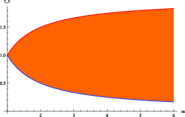
Figure 1: For $d=2$ $(\mu=1)$, the critical mean resource productions $r_{w,c}$ and $r_{s,c}$ are plotted (in blue and in red, resp.), as functions of $m$.

Of course, we realize that the uniform distribution pushes the largest and the smallest order statistics far apart. Therefore, it is informative to look also at a case when the resource claim distribution is more concentrated around its mean, as, for instance, in the case of a beta distribution on $(0,1)$, with parameters $a$ and $b$, say. The distribution function is then defined on $(0,1)$ by the regularized incomplete beta function: $F(x)=I_{a,b}(x)$. The mean resource claim is given by $\mu=\frac{a}{a+b}$. As in Theorems 4.4(a) and 4.7(a), let $r<m\mu=\frac{am}{a+b}$ and suppose that $F(r/k)>0$ for some $k\geq 2$ with $p_{k}>0$.

First, focus on the corresponding w.f.-process. The value of $\tau$ [see equation (7)] is determined by

$$\frac{r}{m} = \int_{0}^{\tau}x\,\mathrm{d}F(x)=\int_{0}^{\tau}\frac{x^{a}(1-x)^{b-1}}{B(a,b)}=\frac{B(a+1,b)}{B(a,b)}I_{a+1,b}(\tau)$$

$$= \frac{a}{a+b}I_{a+1,b}(\tau),$$

which yields $\tau=I^{-1}_{a+1,b}(\frac{r}{m}\frac{a+b}{a})$. The critical mean resource production $r_{w,c}$ is thus defined by

$$mF(\tau)=1\quad\Longleftrightarrow\quad mI_{a,b}\biggl{(}I^{-1}_{a+1,b}\biggl{(}r_{w,c}\frac{a+b}{am}\biggr{)}\biggr{)}=1,$$

which implies

$$r_{w,c}=\frac{am}{a+b}I_{a+1,b}\bigl{(}I_{a,b}^{-1}(1/m)\bigr{)}.$$

Now look at the corresponding s.f.-process. The value of $\theta$ [see equation (9)] is determined by

$$\frac{r}{m}=\int_{\theta}^{1}x\,\mathrm{d}F(x)=\frac{a}{a+b}\bigl{(}1-I_{a+1,b}(\theta)\bigr{)},$$

which yields $\theta=I_{a+1,b}^{-1}(1-\frac{r}{m}\frac{a+b}{a})$. Straightforward calculations then give the critical mean resource production $r_{s,c}=\frac{am}{a+b}(1-I_{a+1,b}(I_{a,b}^{-1}(1-1/m)))$.

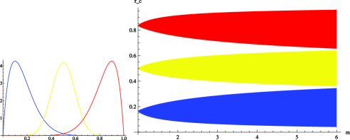
Figure 2: The critical mean resource productions $r_{w,c}$ and $r_{s,c}$ are plotted as functions of $m$, in the case of a $B(a,b)$ resource claim distribution, for typical values of $(a,b)$: $(2,10)$ in blue, $(14,14)$ in yellow and $(10,2)$ in red.

Observing that $I_{\alpha,\beta}(1-x)=1-I_{\beta,\alpha}(x)$, we deduce that $I_{\alpha,\beta}^{-1}(1-x)=1-I_{\beta,\alpha}^{-1}(x)$. The formula for $r_{s,c}$ can thus be rewritten as

$$r_{s,c}=\frac{am}{a+b}I_{b,a+1}\bigl{(}I_{b,a}^{-1}(1/m)\bigr{)}.$$

For a f.c.f.s.-process, the corresponding critical mean resource production simply reads $r_{u,c}=\mu$. Further, for large $m$, we can use the approximation

$$I_{\alpha,\beta}(z)=\frac{z^{\alpha}}{B(\alpha,\beta)}\biggl{(}\frac{1}{\alpha}+\frac{1-\beta}{\alpha+1}z+O\bigl{(}z^{2}\bigr{)}\biggr{)};$$

see, for example, Pearson (1968). Straightforward calculations then give, at leading order,

$$r_{w,c}=\frac{a}{a+1}\biggl{(}\frac{a}{m}B(a,b)\biggr{)}^{1/a}+O\bigl{(}m^{-2/a}\bigr{)},$$

and

$$r_{s,c}=1+\frac{b}{b+1}\bigl{(}b-a(b+1)\bigr{)}\biggl{(}\frac{b}{m}B(b,a)\biggr{)}^{1/b}+O\bigl{(}m^{-2/b}\bigr{)}.$$

Figure 2 shows the critical areas in some typical cases, as the peak is centered, moved to the left or to the right. Figure 3 shows, in the centered case, how the critical area narrows as the dispersion around the peak diminishes.

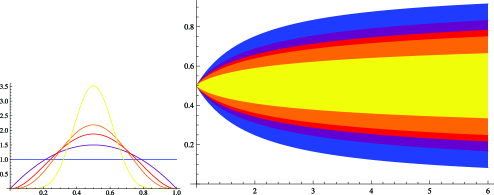
Figure 3: The critical mean resource productions $r_{w,c}$ and $r_{s,c}$ are plotted as functions of $m$, in the case of a $B(a,b)$ resource claim distribution, for different symmetric values of $(a,b)$: $(1,1)$ in blue, $(2,2)$ in pink, $(3,3)$ in red, $(4,4)$ in orange and $(10,10)$ in red.

In the third example we choose a case where resource claims are not bounded. Our results in the s.f.-case can therefore not be used directly but it is interesting to see what happens to the corresponding w.f.-process. Let $F$ be the distribution function of an exponential random variable with parameter $\lambda$. The mean resource claim is given by $\mu=1/\lambda$. As in Theorem 4.4(a), let $r<m\mu=m/\lambda$ and suppose that $F(r/k)>0$ for some $k\geq 2$ with $p_{k}>0$. The value of $\tau$ is determined by [see equation (7)]

$$\frac{r}{m}=\int_{0}^{\tau}x\,\mathrm{d}F(x)=\int_{0}^{\tau}\lambda xe^{-\lambda x}\,\mathrm{d}x=\frac{1}{\lambda}-e\biggl{(}\tau+\frac{1}{\lambda}\biggr{)}e^{-\lambda(\tau+1/\lambda)}$$

which yields $\tau=-\frac{1}{\lambda}(1+\mathrm{W}[-\frac{\lambda}{e}(\frac{1}{\lambda}-\frac{r}{m})])$, where $\mathrm{W}[\cdot]$ denotes the Lambert W function; see, for example, Corless et al. (1996). The critical mean resource production $r_{w,c}$ is thus determined by

$$mF(\tau)=1\quad\Longleftrightarrow\quad m\biggl{(}1-\exp\biggl{(}\mathrm{W}\biggl{[}-\frac{\lambda}{e}\biggl{(}\frac{1}{\lambda}-\frac{r_{w,c}}{m}\biggr{)}\biggr{]}+1\biggr{)}\biggr{)}=1.$$

After simplifications, we get $r_{w,c}=\frac{1}{\lambda}(1-(m-1)\log{(\frac{m}{m-1})})$, where we recall that $\frac{1}{\lambda}=\mu$. For larger $m$, this becomes $r_{w,c}\approx 1/(2\lambda m)=\mu/(2m)$, that is, about one half of what is required for $U[0,1]$-claims.

6 Proofs

6.1 Preliminary results

We first prove Lemma 3.9.

Proof of Lemma 3.9 The property of $M(t,(x_{k})_{k=1}^{t},s)$ being increasing in $s$ is evident from the definition. To see unimodality in $t$, let $I(t,s)=\mathbh 1\{\sum_{j=1}^{t}x_{j,t}\leq s\}$. Then (4) can be written as

$$M\bigl{(}t,(x_{k})_{k=1}^{t},s\bigr{)}=I(t,s)t+\bigl{(}1-I(t,s)\bigr{)}\sup\Biggl{\{}1\leq k\leq t\dvtx\sum_{j=t-k+1}^{t}x_{j,t}\leq s\Biggr{\}},$$

where $\sup\varnothing:=0$. This sum is clearly linearly increasing in $t$ as long as $I(t,s)=1$; it is decreasing in $t$ as soon as $I(t,s)=0$, since the $k$ largest order statistics are increasing with the sample size $t$. Hence, if $t_{1},t_{2}\in\mathbb{N}_{0}$, then, for fixed $s$, $M(t,(x_{k})_{k=1}^{t},s)$ is either monotone increasing or monotone decreasing on $[t_{1},t_{2}]$, or else takes its maximum somewhere in $(t_{1},t_{2})$. This means that $M$ is cap-unimodal in $t$, and hence the minimum

$$\min_{t\in[t_{1},t_{2}]}M\bigl{(}t,(x_{k})_{k=1}^{t},s\bigr{)}$$

is assumed in either $t_{1}$ or $t_{2}$. Finally, the estimate for the corresponding maximum on $[t_{1},t_{2}$] is evident from the definition of $M(t,(x_{k})_{k=1}^{t},s)$.

We now prove Proposition 4.1.

Proof of Proposition 4.1 Let $\pi$ be some policy (in the sense of Definition 2.1). Given $\Gamma_{n}$, the distributions of $D_{n}(\Gamma_{n})$ and $R_{n}(\Gamma_{n})$ are independent from $\Gamma_{1},\ldots,\Gamma_{n-1}$, so that

$$\Gamma_{n+1}=Q^{\pi}\bigl{(}D_{n}(\Gamma_{n}),\bigl{(}X_{n}^{k}\bigr{)}_{k=1}^{D_{n}(\Gamma_{n})},R_{n}(\Gamma_{n})\bigr{)}$$

is independent of $\Gamma_{1},\ldots,\Gamma_{n-1}$, given $\Gamma_{n}$. Thus, $(\Gamma_{n})_{n}$ is a Markov process. Now note that, since $Q^{\pi}(0,\varnothing,s)=0$ and $D_{n}(0)=0$ for all $n\in\mathbb{N}$, we have $\{\Gamma_{n}=0\}\subset\{\Gamma_{n+1}=0\}$ so that $0$ is an absorbing state for the process $(\Gamma_{n})_{n}$. Moreover, since

$$\Gamma_{n+1}=Q^{\pi}\bigl{(}D_{n}(\Gamma_{n}),\bigl{(}X_{n}^{k}\bigr{)}_{k=1}^{D_{n}(\Gamma)},R_{n}(\Gamma_{n})\bigr{)}\leq D_{n}(\Gamma_{n}),$$ (12)

it follows that

$$\mathrm{P}[\Gamma_{n+1}=0|\Gamma_{n}]\geq P\bigl{[}D_{n}(\Gamma_{n})=0|\Gamma_{n}\bigr{]}=p_{0}^{\Gamma_{n}},$$ (13)

where the last equality holds because of the assumption of independent reproduction. Therefore, the absorbing state $0$ is accessible from any state $s\in\mathbb{N}$, with at least probability $p_{0}^{s}>0$. The state $0$ is thus the only absorbing state, and, as $(\Gamma_{n})_{n}$ is a Markov process, we conclude

$$\mathrm{P}[0<\Gamma_{n}\leq s\mbox{ i.o.}]=0\qquad\forall s\in\mathbb{N}_{0}.$$ (14)

The same arguments immediately adapt to multiparameter policies.

We now turn to the proof of Proposition 4.2. The idea is that we compare the behavior of $(W_{n})_{n}$ in each step $n$ with a process consisting of $W_{n}$ i.i.d. versions of a weakest-first process starting with one individual.

Proof of Proposition 4.2 Let $L\in\mathbb{N}_{0}$ and let $W_{n}^{(1)},\ldots,W_{n}^{(L)}$ be $L$ i.i.d. copies of a weakest-first process. We then have the following (superadditivity-type) inequality, namely, for all $n,k\in\mathbb{N}_{0}$,

$$\mathrm{P}[W_{n}\leq k|W_{0}=L]$$

(15)

$$\qquad\leq\mathrm{P}\bigl{[}W_{n}^{(1)}+\cdots+W_{n}^{(L)}\leq k|W_{0}^{(1)}=\cdots=W_{0}^{(L)}=1\bigr{]},$$

which we shall prove first.

To see this, we begin with the case $n=1$.

The case $L=1$ is trivial; hence suppose $L>1$. The LHS of (6.1) becomes, by an additional conditioning on $D_{1}(L)\sim D(L)$,

$$P[W_{1}\leq k|W_{0}=L]$$

$$\qquad=P\bigl{[}D(L)\leq k\bigr{]}+P\bigl{[}W_{1}\leq k|D_{1}(L)>k,W_{0}=L\bigr{]}P\bigl{[}D(L)>k\bigr{]},$$

where we have used the facts that the distribution of $D(L)$ depends only on $L$ (and not on the generation number), and also that $W_{1}$ cannot possibly exceed $D_{1}(W_{0})=D_{1}(L)$.

Now suppose we do the same conditioning on the RHS of (6.1), that is, for the offspring of the $L$ partitioned processes. The first term $P[D(L)\leq k]$ is then the same on both sides, since, as before, reproduction of individuals is independent. Hence, subtracting equal terms on both sides we can now limit our interest to the corresponding second term with more than $k$ offspring.

The distributions of the total created resource space and of the claims are by definition the same on both sides; therefore it suffices to look for the moment at the influence of the order statistics of claims in a fixed sequence of claims on a fixed resource space $R$, say.

In the LHS model of (6.1), the resource space $R$ is global (i.e., united) because all descendants from the different families contribute to a common resource space. In the RHS model of (6.1), this resource space is, however, local (i.e., compartmented). On the LHS the count of individuals to stay is therefore the count of the globally smallest order statistics of claims which can be successively accommodated by $R$ whereas on the RHS the count is on the locally smallest order statistics of claims. The latter, put in increasing order, are a subsequence of the sequence of claims in increasing order. Hence the RHS count cannot exceed the lhs count.

Passing from the counting argument to the corresponding probability measures on both sides proves (6.1) for $n=1$, that is, under the condition $W_{0}=L$ the number of descendants staying in the population is stochastically larger than $W_{1}^{(1)}+\cdots+W_{1}^{(L)}$, that is, for all $j\in\mathbb{N}_{0}$,

$$\mathrm{P}[W_{1}\geq j|W_{0}=L]\geq\mathrm{P}\bigl{[}W_{1}^{(1)}+\cdots+W_{1}^{(L)}\geq j|W_{0}^{(1)}=\cdots=W_{0}^{(L)}=1\bigr{]}.$$

But now, we can iterate this argument. Clearly inequality (6.1) must hold in particular if we replace, on the RHS only, the number $L$ by some $L^{\prime}$ with $L^{\prime}\leq L$. Hence the stochastic order is maintained through the next generation, and thus, by recurrence, through all generations. This implies that (6.1) is true for all $n\in\mathbb{N}_{0}$.

Finally, choosing $k=0$ in (6.1) and taking the limit for $n\to\infty$, we obtain by independence of the processes $(W_{n}^{(j)})_{n}$ that

$$\mathrm{P}[W_{n}\to 0|W_{0}=L]$$

(16)

$$\qquad\leq\mathrm{P}\bigl{[}W_{n}^{(1)}\to 0,\ldots,W_{n}^{(L)}\to 0|W_{0}^{(1)}=\cdots=W_{0}^{(L)}=1\bigr{]}=q_{W}^{L},$$

which completes the proof.

Remark 6.1.

The superadditivity-type inequality (6.1) is in general no longer correct if the w.f.-process is replaced by other RDBPs. Indeed, a very large claim may force on the RHS all the offspring of one subpopulation to leave, but this effect stays still local whereas it may be large on the global LHS. This exemplifies at the same time the adherent difficulty in estimating extinction probabilities for arbitrary policies.

6.2 Uniform bounds

We first prove Proposition 4.3.

Proof of Proposition 4.3 Let $\pi$ be any policy (the same arguments immediately adapt to multiparameter policies). First note that, by definition of $N$ and $M$,

$$M\bigl{(}t,(x_{k})_{k=1}^{t},s\bigr{)}\leq Q^{\pi}\bigl{(}t,(x_{k})_{k=1}^{t},s\bigr{)}\leq N\bigl{(}t,(x_{k})_{k=1}^{t},s\bigr{)}$$

(17)

$$\eqntext{\forall t,\ \forall(x_{k})_{k=1}^{t},\ \forall s.}$$ (18)

We shall now show by induction that if $(\Gamma_{n})_{n}$ is the RDBP controlled by $\pi$, it follows that $\Gamma_{n}\leq W_{n}$ a.s. for all $n$, given $W_{0}=\Gamma_{0}=1$. Indeed, it is true at any time at which the two processes have the same number of individuals, and hence for $n=0$.

Now, if it is true for some $n$, we deduce that, a.s.,

$$\Gamma_{n+1} = Q^{\pi}\bigl{(}D_{n}(\Gamma_{n}),\bigl{(}X_{n}^{k}\bigr{)}_{k=1}^{D_{n}(\Gamma_{n})},R_{n}(\Gamma_{n})\bigr{)}$$ (19)

$$\leq N\bigl{(}D_{n}(\Gamma_{n}),\bigl{(}X_{n}^{k}\bigr{)}_{k=1}^{D_{n}(\Gamma_{n})},R_{n}(\Gamma_{n})\bigr{)}$$ (20)

$$\leq N\bigl{(}D_{n}(W_{n}),\bigl{(}X_{n}^{k}\bigr{)}_{k=1}^{D_{n}(W_{n})},R_{n}(W_{n})\bigr{)}=W_{n+1},$$ (21)

as the mapping $(t,s)\mapsto N(t,(x_{k})_{k=1}^{t},s)$ is increasing in both arguments. Hence the inequality is also true for $n+1$.

It follows that $\mathrm{P}[\Gamma_{n}\leq W_{n}]=1$ for all $n$. Since the limiting extinction probabilities of $(\Gamma_{n})_{n}$ and $(W_{n})_{n}$ must exist, we must also have $q_{W}\leq q_{\Gamma}$.

We now give an explicit counterexample showing that it is in general not true that $S_{n}\leq\Gamma_{n}$ a.s. for all $n$, given $S_{0}=\Gamma_{0}=1$. The underlying idea was already explained in Section 4.2.1.

Counterexample

We have assumed $p_{k}>0$ for some $k\geq 2$ [see regularity assumption (ii) in Section 2.7]; to fix ideas, assume that $p_{3}>0$ (the argument can be adapted in any case). Then consider the deterministic policy $\pi$ given by

$$\pi_{t}\bigl{(}(x_{k})_{k=1}^{t}\bigr{)}(j)=\cases{\sigma(3),&\quad if $j=1$ and $t\geq 3$,\vspace*{2pt}\cr\sigma(1),&\quad if $j=2$ and $t\geq 3$,\vspace*{2pt}\cr\sigma(2),&\quad if $j=3$ and $t\geq 3$,\vspace*{2pt}\cr\sigma(j),&\quad otherwise,}$$ (22)

where $\sigma$ is the permutation such that $x_{\sigma(1)}\geq\cdots\geq x_{\sigma(t)}$ [i.e., by definition, $\sigma=\pi^{S}_{t}((x_{k})_{k=1}^{t})$]. Let, for example,

$$D_{0}^{1} = 3,\qquad X_{0}^{1}>X_{0}^{2}>X_{0}^{3},\qquad X_{0}^{1}+X_{0}^{3}<R_{0}^{1}<X_{0}^{1}+X_{0}^{2},$$

$$D_{1}^{1} = D_{1}^{2}=3,\qquad X_{1}^{1}+X_{1}^{2}+X_{1}^{3}\leq R_{1}^{1}$$

and then

$$X_{1}^{4},X_{1}^{5},X_{1}^{6}>R_{1}^{1}+R_{1}^{2}.$$

These events will occur simultaneously with positive probability, as $p_{3}>0$. But then we immediately see that $\Gamma_{2}=0<3=S_{2}$ in this case.

6.3 Extinction criterion for the w.f.-society

In this section, we will prove Theorem 4.4. In these proofs, we will repeatedly make use of the following lemma, which we shall prove first.

Lemma 6.2

Let $X_{1},X_{2},\ldots$ be i.i.d. real-valued nonnegative random variables with mean $\mu<\infty$ and continuous distribution function $F$. Further, let $(\Phi_{n})_{n}$ be a sequence of integer-valued random variables with $\Phi_{n}\to\infty$ a.s. as $n\to\infty$, and let $(\Psi_{n})_{n}$ be a sequence of real random variables with $\Psi_{n}\to\infty$ a.s. as $n\to\infty$. Suppose that $\Psi_{n}/\Phi_{n}\to\rho$ a.s. with $0<\rho\leq\mu$, and that $\tau$ is the solution of

$$\int_{0}^{\tau}x\,\mathrm{d}F(x)=\rho.$$

Let $N$ be defined by (2). Then $N(\Phi_{n},(X_{k})_{k=1}^{\Phi_{n}},\Psi_{n})/\Phi_{n}\to F(\tau)$ a.s.

Moreover, if the random variables $X_{1},X_{2},\ldots$ are bounded, then we have an analogous result for $M$ defined in (4): defining $\theta$ as the solution of

$$\int_{\theta}^{b}x\,\mathrm{d}F(x)=\rho,$$

then $M(\Phi_{n},(X_{k})_{k=1}^{\Phi_{n}},\Psi_{n})/\Phi_{n}\to 1-F(\theta)$ a.s.

Since $\Psi_{n}/\Phi_{n}\to\rho>0$ a.s. as $n\to\infty$, we have

$$\forall\varepsilon>0\qquad\mathrm{P}\biggl{[}\mathop{\operatorname{sup}}_{n\geq b}\biggl{|}\frac{\Psi_{n}}{\Phi_{n}}-\rho\biggr{|}<\varepsilon\biggr{]}\to 1\qquad\mbox{a.s. as $b\to\infty$.}$$ (23)

To simplify notation, we write $N(t,s):=N(t,(X_{k})_{k=1}^{t},s)$. (Note that this simplification is here admissible since the distribution of the string of claims depends only on $t$.)

As the function $N(t,s)$ is stochastically increasing in $s$, we deduce from almost-sure convergence of $\Phi_{n}/\Psi_{n}$ to $\rho$ that, for all $0\leq\varepsilon<\rho$ and all $\delta>0$, the inequalities

$$\frac{N(\Phi_{n},(\rho-\varepsilon)\Phi_{n})}{\Phi_{n}}\leq\frac{N(\Phi_{n},\Psi_{n})}{\Phi_{n}}\leq\frac{N(\Phi_{n},(\rho+\varepsilon)\Phi_{n})}{\Phi_{n}}$$ (24)

must hold (simultaneously), for all $n$ sufficiently large, with probability at least $1-\delta$.

We now use Theorem 2.2 (on page 615) of Bruss and Robertson (1991). This theorem [refining a result of Coffman, Flatto and Weber (1987)] implies that

$$\frac{N(n,s_{n})}{n}\to F\bigl{(}\tau(s)\bigr{)}\qquad\mbox{a.s. as $n\to\infty$,}$$ (25)

where $\tau(s)$ is the solution of

$$\int_{0}^{\tau(s)}x\,\mathrm{d}F(x)=\lim_{n\to\infty}\frac{s_{n}}{n}=:s,$$ (26)

provided that the latter limit exists and satisfies $0<s\leq\mu=\mathrm{E}[X]$.

Now note that $\tau(\cdot)$ is continuous on $(0,\mu)$ because $F$ is assumed to be continuous on its support.

As $\Phi_{n}\to\infty$ a.s., the left-hand side variable of (24) must converge a.s. to $F(\tau(\rho-\varepsilon))$ and the right-hand side variable of (24) a.s. to $F(\tau(\rho+\varepsilon))$. Since $\varepsilon>0$ is arbitrary and

$$\lim_{\varepsilon\to 0^{+}}F\bigl{(}\tau(\rho\pm\varepsilon)\bigr{)}=F\bigl{(}\tau(\rho)\bigr{)}$$

by continuity of $F(\cdot)$ and $\tau(\cdot)$, the first part of the lemma is proved.

The second part of the lemma, that is, the statement that

$$M\bigl{(}\Phi_{n},(X_{k})_{k=1}^{\Phi_{n}},\Psi_{n}\bigr{)}/\Phi_{n}\to 1-F(\theta)\qquad\mbox{a.s.},$$

can now be proved similarly, using Theorem 2.3 of Bruss and Robertson (1991). Note that we need here, as stated, the assumption that the resource claims are bounded, since the cited Theorem 2.3 may not hold otherwise.

We can now prove Theorem 4.4.

Proof of Theorem 4.4 We first prove statement (a). Suppose $r\leq m\mu$ and $mF(\tau)<1$, and let

$$W^{\infty}(\Omega)=\bigl{\{}\omega\in\Omega\dvtx W_{n}(\omega)\to\infty\mbox{ as $n\to\infty$}\bigr{\}}.$$ (27)

In the following, we can use the shorthand notation $N_{n}(t,s):=N(t,(X_{n}^{k})_{k=1}^{t},\break s)$, where again the index $n$ will be dropped only if the distribution is used.

Now look at

$$\mathrm{E}[W_{n+1}|W_{n}=w]=\mathrm{E}\bigl{[}N_{n}\bigl{(}D_{n}(w),R_{n}(w)\bigr{)}|W_{n}=w\bigr{]}.$$ (28)

Since $R_{n}(w)/w\to r$ a.s. as $w\to\infty$ and $D_{n}(w)/w\to m$ a.s. as $w\to\infty$ and $m>0$, we have $R_{n}(w)/D_{n}(w)\to\rho:=r/m$ a.s. According to Lemma 4.1 (on page 622) of Bruss and Robertson (1991), there exists a sequence $T_{w}\to\tau$ a.s. as $w\to\infty$ with

$$\mathrm{E}\bigl{[}N_{n}\bigl{(}D_{n}(w),R_{n}(w)\bigr{)}|W_{n}=w\bigr{]}\leq\mathrm{E}\bigl{[}D_{n}(w)\bigr{]}F(T_{w}),$$ (29)

where $\tau$ is the solution of

$$\int_{0}^{\tau}x\,\mathrm{d}F(x)=\rho=\frac{r}{m}.$$

Since $F$ is continuous we can find, for each $\varepsilon>0$, a value $w=w(\varepsilon)$ such that $F(T_{v})\leq F(\tau+\varepsilon)$ for all $v\geq w$. Thus, from equations (28) and (29),

$$\mathrm{E}[W_{n+1}|W_{n}=v]\leq mvF(\tau+\varepsilon),\qquad v\geq w.$$ (30)

Hence we get

$$\mathrm{E}[W_{n+1}|W_{n}\geq w] = \sum_{v=w}^{\infty}\mathrm{P}[W_{n}=v|W_{n}\geq w]\mathrm{E}[W_{n+1}|W_{n}=v]$$ (31)

$$\leq mF(\tau+\varepsilon)\sum_{v=w}^{\infty}v\mathrm{P}[W_{n}=v|W_{n}\geq w]$$ (32)

$$= mF(\tau+\varepsilon)\mathrm{E}[W_{n}|W_{n}\geq w].$$ (33)

Since $mF(\tau)<1$, we can choose, again by continuity of $F$, a positive value $\varepsilon$ sufficiently small such that $mF(\tau+\varepsilon)<1$. The latter implies then that $(\mathrm{E}[W_{n}])_{n}$ must be bounded. Consequently, Proposition 4.1 implies that$\mathrm{P}[W^{\infty}(\Omega)]=0$, or equivalently, since $(W_{n})_{n}$ is Markovian, $q_{W}=1$.

This proves the first part of Theorem 4.4(a).

To see the second part of Theorem 4.4(a), we now suppose that $r\leq m\mu$ and $mF(\tau)>1$. Recall that we had supposed that any finite level can be reached with a strictly positive probability [see regularity assumption (iii) in Section 2.7]. Therefore it suffices to show that, for $w$ sufficiently large,

$$\exists\alpha\geq 1\qquad\mathop{\operatorname{liminf}}_{k\to\infty}\mathrm{P}\bigl{[}W_{n+k}\geq\alpha^{k}w|W_{n}\geq w\bigr{]}>0.$$ (34)

Let now

$$h(j,\alpha,w):=\mathrm{P}\bigl{[}W_{n+j}<\alpha^{j}w|W_{n+j-1}\geq\alpha^{j-1}w\bigr{]}.$$ (35)

It follows that

$$\mathrm{P}\bigl{[}W_{n+k}\geq\alpha^{k}w|W_{n}\geq w\bigr{]}$$

(36)

$$\qquad\geq\bigl{(}1-h(k,\alpha,w)\bigr{)}\mathrm{P}\bigl{[}W_{n+k-1}\geq\alpha^{k-1}w|W_{n}\geq w\bigr{]}$$

and thus by recurrence on $k$ that

$$\mathrm{P}\bigl{[}W_{n+k}\geq\alpha^{k}w|W_{n}\geq w\bigr{]}\geq\prod_{j=1}^{k}\bigl{(}1-h(j,\alpha,w)\bigr{)}.$$ (37)

Therefore a sufficient condition for (34) to hold is

$$\sum_{j=1}^{\infty}h(j,\alpha,w)<\infty.$$ (38)

Since $N_{n}(\cdot,\cdot)$, $D_{n+j}(\cdot)$ and $R_{n+j}(\cdot)$ are all stochastically increasing in their arguments, we have

$$h(j,\alpha,w) = \mathrm{P}\bigl{[}W_{n+j}<\alpha^{j}w|W_{n+j-1}\geq\alpha^{j-1}w\bigr{]}$$

$$= \mathrm{P}\bigl{[}N_{n+j}\bigl{(}D_{n+j}(W_{n+j-1}),$$

$$\hskip 10.0ptR_{n+j}(W_{n+j-1})\bigr{)}<\alpha^{j}w|W_{n+j-1}\geq\alpha^{j-1}w\bigr{]}$$

$$\leq \mathrm{P}\bigl{[}N_{n+j}\bigl{(}D_{n+j}\bigl{(}\bigl{\lfloor}\alpha^{j-1}w\bigr{\rfloor}\bigr{)},R_{n+j}\bigl{(}\bigl{\lfloor}\alpha^{j-1}w\bigr{\rfloor}\bigr{)}\bigr{)}<\alpha^{j}w\bigr{]}.$$ (41)

Choose $\varepsilon>0$ such that $(m-\varepsilon)F(\tau)>1$, and put $\alpha=(m-\varepsilon)F(\tau)$. Then we have $p_{0}^{\alpha}<1$ so that

$$\sum_{j=1}^{\infty}p_{0}^{\lfloor\alpha^{j-1}w\rfloor}=\sum_{j=1}^{\infty}\mathrm{P}\bigl{[}D_{n+j}\bigl{(}\bigl{\lfloor}\alpha^{j-1}w\bigr{\rfloor}\bigr{)}=0\bigr{]}<\infty.$$ (42)

Since the $D_{n+j}$ are independent random variables, it follows from the Borel–Cantelli lemma that $\mathrm{P}[D_{n+j}(\lfloor\alpha^{j-1}w\rfloor)=0$ $j$-i.o.$]=0$. Therefore, for $j$ sufficiently large, inequality (41) is equivalent to

$$h(j,\alpha,w)\leq\mathrm{P}\bigl{[}L_{j}^{*}<R_{j}^{*}\bigr{]},$$ (43)

where the LHS variable is defined by

$$L_{j}^{*}=\frac{N_{n+j}(D_{n+j}(\lfloor\alpha^{j-1}w\rfloor),R_{n+j}(\lfloor\alpha^{j-1}w\rfloor))}{D_{n+j}(\lfloor\alpha^{j-1}w\rfloor)}$$ (44)

and the corresponding RHS variable by

$$R_{j}^{*}=\frac{\alpha^{j}w}{D_{n+j}(\lfloor\alpha^{j-1}w\rfloor)}.$$ (45)

Now let $\beta_{j}=\lfloor\alpha^{j-1}w\rfloor$.

First look at the random variables $D_{n+j}(\beta_{j})/\beta_{j}\sim D(\beta_{j})/\beta_{j}$ (and recall that, whenever we drop indices of variables in our notation, then this means that we use information on their distributional prescription only). $D(k)$ is hence distributed like a sum of $k$ i.i.d. random variables with finite mean $m$ and finite variance $\sigma_{D}^{2}$, say.

Recall that $\alpha>1$, and that $\beta_{j}/j\to\infty$ as $j\to\infty$. Therefore, it follows from the Hsu–Robbins theorem of complete convergence [see Theorem 1 of Hsu and Robbins (1947), or Asmussen and Kurtz (1980)] that $D(\beta_{j})/\beta_{j}\to m$ completely as $j\to\infty$. Note that complete convergence holds row-wise in the reproduction matrix since all $D_{k}^{j}$ are i.i.d. and have finite variance. This implies

$$\forall\delta>0\qquad\sum_{j=1}^{\infty}\mathrm{P}\biggl{[}\biggl{|}\frac{D(\beta_{j})}{\beta_{j}}-m\biggr{|}>\delta\biggr{]}<\infty.$$ (46)

Further, since $\alpha^{j}w/\beta_{j}\to\alpha$ as $j\to\infty$ and $D_{n+j}(\cdot)\sim D(\cdot)$, we obtain from (45) and (46)

$$\forall\delta>0\qquad\sum_{j=1}^{\infty}\mathrm{P}\biggl{[}\biggl{|}R_{j}^{*}-\frac{\alpha}{m}\biggr{|}>\delta\biggr{]}<\infty.$$ (47)

Second, to study the convergence of $L_{j}^{*}$ defined in (44) we turn to Lemma 6.2 with $\Phi_{j}=D(\beta_{j})$ and $\Psi_{j}=R(\beta_{j})$. Since $\Phi_{j}/\beta_{j}\to m$ completely and $\Psi_{j}/\beta_{j}\to r$ completely (again by the Hsu–Robbins theorem), we have

$$\frac{\Psi_{j}}{\Phi_{j}}\to\rho=\frac{r}{m}\qquad\mbox{completely, as $j\to\infty$.}$$ (48)

Therefore, in particular, $\Psi_{j}/\Phi_{j}\to\rho$ a.s., so that the conditions of Lemma 6.2 are satisfied. It follows that if $L_{j}^{*}$ in (44) allows for a limit (in some sense) $l$, say, then we must have $l=F(\tau)$, where $\tau$ is defined as in Lemma 6.2.

Using this and the Chernov-type estimates obtained by Coffman, Flatto and Weber (1987) (see Theorems 2 and 3) with $a=j\delta$, we obtain after some straightforward simplifications,

$$\mathrm{P}\biggl{[}\biggl{|}\frac{N(\cdot,\cdot)}{j}-F(\tau)\biggr{|}>\delta\biggr{]}\leq 2e^{-({j\delta^{2}})/({4F(\tau)})}.$$ (49)

Again $N_{n+j}(\cdot,\cdot)\sim N(\cdot,\cdot)$ and $\beta_{j}/j\to\infty$, and thus $L_{j}^{*}\to F(\tau)$ completely as $j\to\infty$. This implies the convergence

$$\forall\delta>0\qquad\sum_{j=1}^{\infty}\mathrm{P}\bigl{[}\bigl{|}L_{j}^{*}-F(\tau)\bigr{|}>\delta\bigr{]}<\infty.$$ (50)

Now choose $\delta=\frac{1}{2}|F(\tau)-\alpha/m|>0$. Note that the event $\{L_{j}^{*}<R_{j}^{*}\}$ can only occur if $|L_{j}^{*}-F(\tau)|>\delta$ or $|R_{j}-\alpha/m|>\delta$. Therefore, from (43),

$$h(j,\alpha,w) \leq \mathrm{P}\bigl{[}L_{j}^{*}<R_{j}^{*}\bigr{]}$$ (51)

$$\leq \mathrm{P}\bigl{[}\bigl{|}L_{j}^{*}-F(\tau)\bigr{|}>\delta\bigr{]}+\mathrm{P}\biggl{[}\biggl{|}R_{j}^{*}-\frac{\alpha}{m}\biggr{|}>\delta\biggr{]}$$ (52)

so that, according to (47) and (50),

$$\sum_{j=1}^{\infty}h(j,\alpha,w)<\infty.$$ (53)

This completes the proof of statement (a).

Statement (b) is obtained similarly (and more easily) using Theorem 2.1 of Bruss and Robertson (1991).

Finally, using Lemma 6.2, it is clear that, if $r\leq m\mu$ and $mF(\tau)>1$, conditioning on survival, we have $W_{n+1}/W_{n}\to mF(\tau)$ a.s. as $n\to\infty$, and thus, for any $\varepsilon,\delta>0$, there exists some large $L_{\varepsilon,\delta}>0$ such that

$$\mathrm{P}\biggl{[}\sup_{n\geq L_{\varepsilon,\delta}}\biggl{|}\frac{W_{n+1}}{W_{n}}-mF(\tau)\biggr{|}<\delta\Big{|}\lim_{n\to\infty}W_{n}=\infty\biggr{]}\geq 1-\varepsilon.$$ (54)

This precisely means that, conditioning on survival, the w.f.-process behaves more and more like a GWP with the modified reproduction mean $\tilde{m}=mF(\tau)$.

6.4 Extinction criterion for the s.f.-society (first part)

In this section, we are concerned with the proof of Theorem 4.7. The first part of Theorem 4.7(a) can be obtained by similar considerations as for Theorem 4.4 (the extinction criterion for the w.f.-society), the role of $\tau$ being now played by $\theta$, defined by

$$\int_{\theta}^{b}x\,\mathrm{d}F(x)=\frac{r}{m},$$

as in Theorem 2.3 of Bruss and Robertson (1991). However, here we need the assumption that the resource claims are bounded as assumed in the model, simply because the cited Theorem 2.3 may not hold otherwise. (This was not needed in the case of the w.f.-society where we only used that the claims have a finite variance.)

Proof of Theorem 4.7(a)(i) The proof of the first part of Theorem 4.7(a) follows the same reasoning as for Theorem 4.4 [see equations (27)–(33)] and yields correspondingly that, for all $\varepsilon>0$, there exists a sufficiently large $s$ such that

$$\mathrm{E}[S_{n+1}|S_{n}\geq s]\leq m\bigl{(}1-F(\theta-\varepsilon)\bigr{)}\mathrm{E}[S_{n}|S_{n}\geq s].$$ (55)

Choosing $\varepsilon$ sufficiently small such that $m(1-F(\theta-\varepsilon))<1$ shows that $(\mathrm{E}[S_{n+1}|S_{n}\geq s])_{n}$ is bounded, so that $(\mathrm{E}[S_{n}])_{n}$ is bounded too. Hence, similarly as before, $q_{S}=1$.

For the other parts of Theorem 4.7, adapting the proof of Theorem 4.4 seems difficult. The major technical difficulty is that we have to deal with the cap-unimodality of $M(\cdot,\cdot)$ in its first argument [while $N(\cdot,\cdot)$ was increasing in both arguments].

Cap-unimodality implies that the minimum of $M(D(t),R(t))$ for given $D(t)$ and $R(t)$ over an interval $[t_{1},t_{2}]$ must be taken on the border, but gives less information about the corresponding maximum. The estimate $t_{2}-t_{1}$ for the difference between the maximum and the minimum over $[t_{1},t_{2}]$ (see Lemma 3.9) is here too crude. We therefore have to proceed differently, and, in order to use arguments developed later, the rest of this proof is postponed to Section 6.8.

6.5 Corollaries 4.6 and 4.9

We shall need the following two lemmas, which we prove first:

Lemma 6.3

Assume $r>\mu$, and let $\tau$ be defined by

$$\int_{0}^{\tau}x\,\mathrm{d}F(x)=\frac{r}{m}.$$

Then $mF(\tau)>1$.

Let $a\geq 0$ be the infimum of the support of $F$. As $F(x)>0$ for all $x>a$ and as $\tau>a$ [because $\int_{0}^{\tau}x\,\mathrm{d}F(x)=\frac{r}{m}>\frac{\mu}{m}\geq 0$], we deduce $F(\tau)>0$, and we can write

$$mF(\tau)\int_{0}^{\tau}x\frac{\mathrm{d}F(x)}{F(\tau)}=r>\mu,$$

or equivalently,

$$mF(\tau)\mathrm{E}[X|X\leq\tau]>\mu.$$

However, $\mathrm{E}[X|X\leq\tau]\leq\mathrm{E}[X]=\mu$, so that the above inequality cannot hold unless $mF(\tau)>1$.

Lemma 6.4

Assume $r<\mu$, and let $\theta$ be defined by

$$\int_{\theta}^{\infty}x\,\mathrm{d}F(x)=\frac{r}{m}.$$

Then $m(1-F(\theta))<1$.

Let $b\geq 0$ be the least upper bound of claims. As $1-F(x)>0$ for all $x<b$ and as $\theta<b$ [because $\int_{\theta}^{\infty}x\,\mathrm{d}F(x)=\frac{r}{m}>0$], we deduce $1-F(\theta)>0$, and we can write

$$m\bigl{(}1-F(\theta)\bigr{)}\int_{\theta}^{\infty}x\frac{\mathrm{d}F(x)}{1-F(\theta)}=r<\mu,$$

or equivalently

$$m\bigl{(}1-F(\theta)\bigr{)}\mathrm{E}[X|X>\theta]<\mu.$$

However, $\mathrm{E}[X|X>\theta]\geq\mathrm{E}[X]=\mu$, so that the above inequality implies $m(1-F(\theta))<1$.

We can now prove Corollary 4.6.

Proof of Corollary 4.6 Using Lemma 6.3 and Theorem 4.4(a)(ii), part (a) is immediate. It remains to prove part (b). Using the Cauchy–Schwarz inequality, we deduce directly from the definition of $\tau$,

$$\frac{r}{m} = \int_{0}^{\tau}x\,\mathrm{d}F(x)=\mu-\int_{\tau}^{b}x\,\mathrm{d}F(x)$$ (56)

$$\geq \mu-\sqrt{1-F(\tau)}\sqrt{\int_{\tau}^{b}x^{2}\,\mathrm{d}F(x)}\geq\mu-\sqrt{1-F(\tau)}\sqrt{\mathrm{E}\bigl{[}X^{2}\bigr{]}},$$ (57)

so that, after straightforward simplifications, $mF(\tau)\leq m-(m\mu-r)^{2}/\break(m\mathrm{E}[X^{2}])$. Hence, if

$${\mathrm{E}\bigl{[}X^{2}\bigr{]}}<(m\mu-r)^{2}/\bigl{(}m(m-1)\bigr{)},$$

we deduce $mF(\tau)<1$ and thus, by Theorem 4.4(a)(i), we must have $q_{W}=1$.

We now turn to the proof of Corollary 4.9.

Proof of Corollary 4.9 Using Lemma 6.4 and Theorem 4.7(a)(i), part (a) is immediate.

It remains to prove part (b).

Using the Cauchy–Schwarz inequality, we deduce directly from the definition of $\theta$

$$\qquad\frac{r}{m} = \int_{\theta}^{b}x\,\mathrm{d}F(x)\leq\sqrt{1-F(\theta)}\sqrt{\int_{\theta}^{b}x^{2}\,\mathrm{d}F(x)}\leq\sqrt{1-F(\theta)}\sqrt{\mathrm{E}\bigl{[}X^{2}\bigr{]}}.$$ (58)

Hence, if ${\mathrm{E}[X^{2}]}<r^{2}/m$, we deduce

$$m\bigl{(}1-F(\theta)\bigr{)}\geq r^{2}/\bigl{(}m\mathrm{E}\bigl{[}X^{2}\bigr{]}\bigr{)}>1$$

and thus, by Theorem 4.7(a)(ii), we must have $q_{S}<1$.

6.6 Conditional envelopment theorem

We prove here Proposition 4.12.

Proof of Proposition 4.12 Assume that $\Gamma_{n}\to\infty$ is given, that is, that $\underline{\gamma}>0$ is given. First compare the process $(\Gamma_{n})_{n}$ with $(S_{n})_{n}$. We see from the corresponding counting functions $Q^{\pi}$ and $M$ that

$$\underline{\gamma} = \liminf_{n\to\infty}\frac{\Gamma_{n+1}}{\Gamma_{n}}=\liminf_{n\to\infty}\frac{Q^{\pi}_{n}(D_{n}(\Gamma_{n}),R_{n}(\Gamma_{n}))}{\Gamma_{n}}$$ (59)

$$\geq \liminf_{n\to\infty}\frac{M_{n}(D_{n}(\Gamma_{n}),R_{n}(\Gamma_{n}))}{\Gamma_{n}},$$ (60)

where the last inequality follows from the definition of the function $M$. Since the latter is increasing in the second argument and cap-unimodal in the first argument, we define (neglecting the floor–roof symbols which are here of no importance)

$$\qquad\widetilde{M}^{\varepsilon}_{n}(\Gamma_{n})=\min\bigl{\{}M_{n}\bigl{(}(m-\varepsilon)\Gamma_{n},(r-\varepsilon)\Gamma_{n}\bigr{)},M_{n}\bigl{(}(m+\varepsilon)\Gamma_{n},(r-\varepsilon)\Gamma_{n}\bigr{)}\bigr{\}},$$ (61)

so that, for all $0<\varepsilon<\min(r,m)$,

$$\underline{\gamma}\geq\liminf_{n\to\infty}\frac{1}{\Gamma_{n}}\widetilde{M}^{\varepsilon}_{n}(\Gamma_{n})=\liminf_{n\to\infty}\frac{m}{D_{n}(\Gamma_{n})}\widetilde{M}^{\varepsilon}_{n}(\Gamma_{n}).$$ (62)

Now, let $\theta^{-}_{\varepsilon}$ and $\theta^{+}_{\varepsilon}$ be defined, respectively, by

$$\int_{\theta_{\varepsilon}^{-}}^{\infty}x\,\mathrm{d}F(x)=\frac{r-\varepsilon}{m-\varepsilon}\quad\mbox{and}\quad\int_{\theta_{\varepsilon}^{+}}^{\infty}x\,\mathrm{d}F(x)=\frac{r-\varepsilon}{m+\varepsilon}.$$ (63)

Then, from Lemma 6.2, we get

$$\frac{\widetilde{M}^{\varepsilon}_{n}(\Gamma_{n})}{D_{n}(\Gamma_{n})}\geq\min\bigl{\{}1-F\bigl{(}\theta_{\varepsilon}^{-}\bigr{)},1-F\bigl{(}\theta_{\varepsilon}^{+}\bigr{)}\bigr{\}},$$ (64)

for all sufficiently large $n$. Hence, using equations (62) and (64), as well as the continuity of $\theta_{\varepsilon}^{-}$ and $\theta_{\varepsilon}^{+}$ as functions of $\varepsilon$, we deduce

$$\underline{\gamma}\geq m\bigl{(}1-F(\theta)\bigr{)}.$$ (65)

Second, we must compare $(\Gamma_{n})_{n}$ with $(W_{n})_{n}$. This is done similarly and more easily because $N(\cdot,\cdot)$ is monotone increasing in both arguments. This yields then directly the other stated inequality $\bar{\gamma}\leq mF(\tau)$ and the proof is complete.

6.7 Unconditional envelopment theorem

In this section, we are concerned with the proof of Theorem 4.13. In the case when $r\leq m\mu$, we define $\tau$ and $\theta$ as in the statement of Theorems 4.4 and 4.7. When $r>m\mu$, these are not defined, but, to simplify notations, we then define $F(\tau):=1$ and $1-F(\theta):=1$.

First of all, we shall need the following interesting result, which is a far-reaching strengthening of equation (54):

Theorem 6.5

For any $\varepsilon>0$ and any $\delta>0$, there exists some sufficiently large $L_{\varepsilon,\delta}>0$ such that, if $mF(\tau)>1$,

$$\mathrm{P}\biggl{[}\sup_{l\geq 0}\biggl{|}\frac{W_{n+l+1}}{W_{n+l}}-mF(\tau)\biggr{|}<\delta\Big{|}W_{n}\geq L_{\varepsilon,\delta}\biggr{]}\geq 1-\varepsilon,$$

and similarly, if $m(1-F(\theta))>1$,

$$\mathrm{P}\biggl{[}\sup_{l\geq 0}\biggl{|}\frac{S_{n+l+1}}{S_{n+l}}-m\bigl{(}1-F(\theta)\bigr{)}\biggr{|}<\delta\Big{|}S_{n}\geq L_{\varepsilon,\delta}\biggr{]}\geq 1-\varepsilon.$$

It should be noted that this result constitutes a new proof of part (a)(ii) of Theorem 4.4, and it will be used to deduce part (a)(ii) of Theorem 4.7 in the next section. In order to prove this result, we shall crucially make use of the following Chernov-type estimates, which we prove first, based on Theorems 2 and 3 of Coffman, Flatto and Weber (1987):

Lemma 6.6

For any $\delta>0$, there exists constants $C,c>0$ such that, for all $n,j\geq 0$,

$$\mathrm{P}\biggl{[}\biggl{|}\frac{W_{n+1}}{W_{n}}-mF(\tau)\biggr{|}>\delta\Big{|}W_{n}=j\biggr{]}\leq Ce^{-cj},$$ (66)

and similarly,

$$\mathrm{P}\biggl{[}\biggl{|}\frac{S_{n+1}}{S_{n}}-m\bigl{(}1-F(\theta)\bigr{)}\biggr{|}>\delta\Big{|}S_{n}=j\biggr{]}\leq Ce^{-cj}.$$ (67)

By definition,

$$\mathrm{P}\biggl{[}\biggl{|}\frac{W_{n+1}}{W_{n}}-mF(\tau)\biggr{|}>\delta\Big{|}W_{n}=j\biggr{]}$$

(68)

$$\qquad=\mathrm{P}\biggl{[}\biggl{|}\frac{N_{n}(D_{n}(j),R_{n}(j))}{j}-mF(\tau)\biggr{|}>\delta\biggr{]}.$$

Let $\eta>0$. As $N_{n}:=N_{n}(\cdot,\cdot)$ is increasing in both arguments, conditioning on $|R_{n}(j)/j-r|\leq\eta$ (resp., $>\eta$) and on $|D_{n}(j)/j-m|\leq\eta$ (resp., $>\eta$) in the RHS, we obtain, after several elementary transformations, that the latter rhs is bounded above by

$$\mathrm{P}\biggl{[}\biggl{|}\frac{N_{n}(j(m+\eta),j(r+\eta))}{j}-mF(\tau)\biggr{|}>\delta\biggr{]}$$

$$\quad{}+\mathrm{P}\biggl{[}\biggl{|}\frac{N_{n}(j(m-\eta),j(r-\eta))}{j}-mF(\tau)\biggr{|}>\delta\biggr{]}$$ (69)

$$\quad{}+\mathrm{P}\biggl{[}\biggl{|}\frac{D_{n}(j)}{j}-m\biggr{|}>\eta\biggr{]}+\mathrm{P}\biggl{[}\biggl{|}\frac{R_{n}(j)}{j}-r\biggr{|}>\eta\biggr{]}.$$

Choosing $\eta$ small enough such that $|(m+\eta)F(\tau((r+\eta)/(m+\eta)))-mF(\tau)|<\delta/2$, the first term of (6.7) becomes smaller than

$$\mathrm{P}\biggl{[}\biggl{|}\frac{N_{n}(j(m+\eta),j(r+\eta))}{j}-(m+\eta)F\biggl{(}\tau\biggl{(}\frac{r+\eta}{m+\eta}\biggr{)}\biggr{)}\biggr{|}>\frac{\delta}{2}\biggr{]}$$

(70)

$$\qquad\leq 2\exp\biggl{(}-\frac{\delta^{2}j}{16mF(\tau)+8\delta}\biggr{)},$$

where the last inequality follows from Theorems 2 and 3 of Coffman, Flatto and Weber (1987). The second term of (6.7) can be bounded similarly.

The two last terms also satisfy an exponential bound by Hoeffding’s inequality [see Theorem 2 of Hoeffding (1963)], since the random variables $D_{n}^{k}$ and $R_{n}^{k}$ are assumed to be bounded. This proves the result in the weakest-first case.

As far as the strongest-first case is concerned, now using the cap-unimodality as well as a simple bound for the minimum and the maximum of $M_{n}$ over the respective intervals (see Lemma 3.9), we can deduce a bound similar to (6.7) (with some additional terms), and the result will follow in an analogous way.

The following result constitutes a first step in the proof of Theorem 6.5:

Proposition 6.7

For any $\varepsilon>0$ and any $\delta>0$, there exists some sufficiently large $L_{\varepsilon,\delta}>0$ such that, if $mF(\tau)>1$,

$$\mathrm{P}\biggl{[}\bigcap_{l\geq 0}\biggl{\{}\frac{W_{n+l+1}}{W_{n+l}}>mF(\tau)-\delta\biggr{\}}\Big{|}W_{n}\geq L_{\varepsilon,\delta}\biggr{]}\geq 1-\varepsilon,$$

and similarly, if $m(1-F(\theta))>1$,

$$\mathrm{P}\biggl{[}\bigcap_{l\geq 0}\biggl{\{}\frac{S_{n+l+1}}{S_{n+l}}>m\bigl{(}1-F(\theta)\bigr{)}-\delta\biggr{\}}\Big{|}S_{n}\geq L_{\varepsilon,\delta}\biggr{]}\geq 1-\varepsilon.$$

Choose $1<\tilde{m}<mF(\tau)$, and take $\delta=mF(\tau)-\tilde{m}>0$. Then we can write the following inequalities, for any $L>0$ and any $n\geq 0$:

$$\mathrm{P}\biggl{[}\frac{W_{n+l+1}}{W_{n+l}}>\tilde{m},\ \forall l\geq 0\Big{|}W_{n}\geq L\biggr{]}$$ (71)

$$\qquad=1-\sum_{l=0}^{\infty}\mathrm{P}[W_{n+j+1}>\tilde{m}W_{n+j}$$

(72)

$$\hskip 75.0pt\mbox{ for all $0\leq j<l$, and }W_{n+l+1}\leq\tilde{m}W_{n+l}|W_{n}\geq L]$$

$$\qquad\geq 1-\sum_{l=0}^{\infty}\mathrm{P}\biggl{[}W_{n+j+1}>\tilde{m}W_{n+j}$$

(73)

$$\hskip 77.0pt\mbox{ for all $0\leq j<l$, and }\biggl{|}\frac{W_{n+l+1}}{W_{n+l}}-mF(\tau)\biggr{|}\geq\delta\Big{|}W_{n}\geq L\biggr{]},$$

since $\tilde{m}=mF(\tau)-\delta$. Now, given $W_{n}\geq L$, the inequalities $W_{n+j+1}>\tilde{m}W_{n+j}$ for all $0\leq j<l$ imply that $W_{n+l}\geq\tilde{m}^{l}L$. Using this and dropping the intersection yields

$$\mathrm{P}\biggl{[}\frac{W_{n+l+1}}{W_{n+l}}>\tilde{m},\ \forall l\geq 0\Big{|}W_{n}\geq L\biggr{]}$$ (74)

$$\qquad\geq 1-\sum_{l=0}^{\infty}\mathrm{P}\biggl{[}\biggl{|}\frac{W_{n+l+1}}{W_{n+l}}-mF(\tau)\biggr{|}\geq\delta\Big{|}W_{n+l}\geq\tilde{m}^{l}L\biggr{]}$$ (75)

$$\qquad\geq 1-\sum_{l=0}^{\infty}\sum_{j=\tilde{m}^{l}L}^{\infty}\mathrm{P}\biggl{[}\biggl{|}\frac{W_{n+l+1}}{W_{n+l}}-mF(\tau)\biggr{|}\geq\delta\Big{|}W_{n+l}=j\biggr{]}$$

(76)

$$\qquad\geq 1-C\sum_{l=0}^{\infty}\sum_{j=\tilde{m}^{l}L}^{\infty}e^{-cj},$$

where the last inequality follows from the Chernov-type estimates given in Lemma 6.6. Now, since $\tilde{m}>1$, a straightforward calculation yields

$$\sum_{l=0}^{\infty}\sum_{j=\tilde{m}^{l}L}^{\infty}e^{-cj} = \sum_{l=0}^{\infty}e^{-c\tilde{m}^{l}L}\sum_{j=0}^{\infty}e^{-cj}=\frac{1}{1-e^{-c}}\sum_{l=0}^{\infty}e^{-c\tilde{m}^{l}L}$$ (77)

$$\leq \frac{1}{1-e^{-c}}e^{-cL}\sum_{l=0}^{\infty}e^{-c(\tilde{m}^{l}-1)}\leq Ke^{-cL},$$ (78)

where the constant $K<\infty$ only depends on $c$ and on $\tilde{m}$. Taking $L$ large enough thus yields the result. The same argument holds in the strongest-first case.

Now using Proposition 6.7, the proof of Theorem 6.5 becomes straightforward:

Proof of Theorem 6.5 Let $n$ be fixed and choose $0<\delta<mF(\tau)-1$. First consider the event

$$\Omega_{\varepsilon,\delta,L}=\biggl{\{}\frac{W_{n+l+1}}{W_{n+l}}>mF(\tau)-\delta\mbox{ for all $l\geq 0$, and }W_{n}\geq L\biggr{\}}\subset\Omega,$$ (79)

for any $L>0$. Proposition 6.7 means that $\mathrm{P}[\Omega_{\varepsilon,\delta,L}]\geq(1-\varepsilon)\mathrm{P}[W_{n}\geq L]$ whenever $L\geq L_{\varepsilon,\delta}$. On $\Omega_{\varepsilon,\delta,L}$, it is clear that $W_{n+l}\to\infty$ a.s. as $l\to\infty$, and Lemma 6.2 then implies that $W_{n+l+1}/W_{n+l}\to mF(\tau)$ a.s. as $l\to\infty$. Hence, there exists a sufficiently large $K_{\varepsilon,\delta}\geq 0$ such that

$$\mathrm{P}\biggl{[}\Omega_{\varepsilon,\delta,L}\cap\biggl{\{}\sup_{l\geq K_{\varepsilon,\delta}}\biggl{|}\frac{W_{n+l+1}}{W_{n+l}}-mF(\tau)\biggr{|}<\delta\biggr{\}}\biggr{]} \geq (1-\varepsilon)\mathrm{P}[\Omega_{\varepsilon,\delta,L}].$$ (80)

Choose such a $K_{\varepsilon,\delta}$. Then, since, for any fixed $k$, Lemma 6.2 gives $N_{k}(D_{k}(j),\break R_{k}(j))/j\to mF(\tau)$ a.s. as $j\to\infty$, we deduce that, for some sufficiently large $L^{\prime}_{\varepsilon,\delta}>0$,

$$\mathrm{P}\biggl{[}\sup_{0\leq l<K_{\varepsilon,\delta}}\biggl{|}\frac{W_{n+l+1}}{W_{n+l}}-mF(\tau)\biggr{|}<\delta\Big{|}W_{n+l}\geq L^{\prime}_{\varepsilon,\delta},\mbox{ for all $0\leq l<K_{\varepsilon,\delta}$}\biggr{]}$$

(81)

$$\qquad\geq 1-\varepsilon.$$

Now note that, whenever $L\geq L^{\prime}_{\varepsilon,\delta}$, we have on $\Omega_{\varepsilon,\delta,L}$ the inequality $W_{n+l}\geq L^{\prime}_{\varepsilon,\delta}$ for all $0\leq l<K_{\varepsilon,\delta}$, so that equation (6.7) yields, for any $L\geq L^{\prime}_{\varepsilon,\delta}$,

$$\mathrm{P}\biggl{[}\Omega_{\varepsilon,\delta,L}\cap\biggl{\{}\sup_{0\leq l<K_{\varepsilon,\delta}}\biggl{|}\frac{W_{n+l+1}}{W_{n+l}}-mF(\tau)\biggr{|}<\delta\biggr{\}}\biggr{]}$$

(82)

$$\qquad\geq(1-\varepsilon)\mathrm{P}[\Omega_{\varepsilon,\delta,L}].$$

We can thus conclude, for $L^{\prime\prime}_{\varepsilon,\delta}=\max(L_{\varepsilon,\delta},L^{\prime}_{\varepsilon,\delta})$, using, for instance, the Bonferroni inequality,

$$\mathrm{P}\biggl{[}\sup_{l\geq 0}\biggl{|}\frac{W_{n+l+1}}{W_{n+l}}-mF(\tau)\biggr{|}<\delta,\mbox{ and }W_{n}\geq L^{\prime\prime}_{\varepsilon,\delta}\biggr{]}$$

(83)

$$\qquad\geq\bigl{(}2(1-\varepsilon)-1\bigr{)}\mathrm{P}[\Omega_{\varepsilon,\delta,L^{\prime\prime}_{\varepsilon,\delta}}]$$

$$\qquad\geq(1-2\varepsilon)(1-\varepsilon)\mathrm{P}\bigl{[}W_{n}\geq L^{\prime\prime}_{\varepsilon,\delta}\bigr{]}.$$ (84)

Replacing $\varepsilon$ by $\varepsilon/3$ yields the result. The same argument holds in the strongest-first case.

We can now turn to the proof of Theorem 4.13.

For that purpose, we first prove the following result, which is interesting in itself:

Proposition 6.8

Let $(\Gamma_{n})_{n}$ be any RDBP. Assume that $m(1-F(\theta))>1$. Then, for any $\varepsilon,\delta>0$, there exists some sufficiently large $L_{\varepsilon,\delta}>0$ such that, for all $n\geq 0$,

$$\mathrm{P}\biggl{[}\bigcap_{l\geq 0}\biggl{\{}\frac{\Gamma_{n+l+1}}{\Gamma_{n+l}}\geq\frac{S_{n+l+1}}{S_{n+l}}-\delta\biggr{\}}\Big{|}\Gamma_{n}=S_{n}\geq L_{\varepsilon,\delta}\biggr{]}\geq 1-\varepsilon.$$

Choose $\tilde{m}=m(1-F(\theta))-\delta/2$ and take $\delta$ small enough so that $\tilde{m}>1$. Then we can write the following inequalities, similarly as in the proof of Proposition 6.7:

$$\mathrm{P}\biggl{[}\frac{\Gamma_{n+l+1}}{\Gamma_{n+l}}>\tilde{m},\ \forall l\geq 0\Big{|}\Gamma_{n}\geq L\biggr{]}$$ (85)

$$\qquad=1-\sum_{l=0}^{\infty}\mathrm{P}[\Gamma_{n+j+1}>\tilde{m}\Gamma_{n+j}$$

(86)

$$\hskip 75.0pt\mbox{ for all $0\leq j<l$, and }\Gamma_{n+l+1}\leq\tilde{m}\Gamma_{n+l}|\Gamma_{n}\geq L]$$

$$\qquad\geq 1-\sum_{l=0}^{\infty}\mathrm{P}\bigl{[}\Gamma_{n+l+1}\leq\tilde{m}\Gamma_{n+l}|\Gamma_{n+l}\geq\tilde{m}^{l}L\bigr{]}$$ (87)

$$\qquad\geq 1-\sum_{l=0}^{\infty}\sum_{j=\tilde{m}^{l}L}^{\infty}\mathrm{P}[\Gamma_{n+l+1}\leq\tilde{m}\Gamma_{n+l}|\Gamma_{n+l}=j].$$ (88)

Now note that, given $\Gamma_{n+l}=S_{n+l}=j$, we have

$$S_{n+l+1}=M_{n+l}\bigl{(}D_{n+l}(j),R_{n+l}(j)\bigr{)}\leq Q^{\Gamma}_{n+l}\bigl{(}D_{n+l}(j),R_{n+l}(j)\bigr{)}\leq\Gamma_{n+l+1}.$$

Using this and the Chernov-type estimates given in Lemma 6.6, we see that for any $\varepsilon>0$, we can find a sufficiently large $L_{\varepsilon,\delta}>0$ such that

$$\mathrm{P}\biggl{[}\frac{\Gamma_{n+l+1}}{\Gamma_{n+l}}>\tilde{m},\ \forall l\geq 0\Big{|}\Gamma_{n}\geq L_{\varepsilon,\delta}\biggr{]}$$

(89)

$$\qquad\geq 1-\sum_{l=0}^{\infty}\sum_{j=\tilde{m}^{l}L}^{\infty}\mathrm{P}[S_{n+l+1}\leq\tilde{m}S_{n+l}|S_{n+l}=j]$$

$$\qquad\geq 1-C\sum_{l=0}^{\infty}\sum_{j=\tilde{m}^{l}L_{\varepsilon,\delta}}^{\infty}e^{-cj}\geq 1-\varepsilon,$$ (90)

where we argued in the second inequality exactly as in the proof of Proposition 6.7. Putting this together with Theorem 6.5 yields the result.

We can now immediately deduce Theorem 4.13:

Proof of Theorem 4.13 On the one hand, if $m(1-F(\theta))>1$, Proposition 6.8 yields

$$\lim_{L\to\infty}\mathrm{P}\Bigl{[}\lim_{n\to\infty}\Gamma_{n}(L)\geq\lim_{n\to\infty}S_{n}(L)\Bigr{]}=1.$$ (91)

On the other hand, if $m(1-F(\theta))<1$, then we have proven that $S_{n}(L)\to 0$ almost surely for any $L>0$ [see Theorem 4.7(a)(i)], and thus equation (91) holds trivially. Finally, using Proposition 4.3 for the upper bound for $(\Gamma_{n})_{n}$ yields, as desired,

$$\lim_{L\to\infty}\mathrm{P}\Bigl{[}\lim_{n\to\infty}S_{n}(L)\leq\lim_{n\to\infty}\Gamma_{n}(L)\leq\lim_{n\to\infty}W_{n}(L)\Bigr{]}=1.$$ (92)

It remains to prove that $q_{W}=1\Rightarrow q_{\Gamma}=1\Rightarrow q_{S}=1$. The first implication simply follows from Proposition 4.3. Now, assuming $q_{\Gamma}=1$, we easily deduce, using the regularity assumption (iii) of Section 2.7, that, for any $L$, we have $\Gamma_{n}(L)\to 0$ a.s., as $n\to\infty$. Hence, equation (92) gives $\mathrm{P}[\lim_{n}S_{n}(L)=0]\to 1$, as $L\to\infty$. It follows then that $q_{S}=1$, as we can show by contradiction, using again the regularity assumption (iii).

6.8 Extinction criterion for the s.f.-society (second part)

In this section, we finish the proof of Theorem 4.7, using the results of previous section (in particular, Theorem 6.5). Therefore, we will need the boundedness assumption for all the random variables $D_{n}^{k}$, $X_{n}^{k}$ and $R_{n}^{k}$ [see regularity assumption (v) of Section 2.7], while only the boundedness of the $X_{n}^{k}$’s was needed for the first part of the proof in Section 6.4.

Proof of Theorem 4.7 The first part of Theorem 4.7(a) has already been proven in Section 6.4.

Now look at the second part, assuming $r\leq m\mu$ and $m(1-F(\theta))>1$. Then, Theorem 6.5 (or Proposition 6.7) gives, for any $\varepsilon>0$ and for $\delta>0$ with $m(1-F(\theta))>1+\delta$,

$$\qquad 1-q_{S} \geq \mathrm{P}\biggl{[}\bigcap_{l\geq 0}\biggl{\{}\frac{S_{n+l+1}}{S_{n+l}}>m\bigl{(}1-F(\theta)\bigr{)}-\delta\biggr{\}}\biggr{]}\geq(1-\varepsilon)\mathrm{P}[S_{n}\geq L_{\varepsilon,\delta}],$$ (93)

so that, using the regularity assumption (iii) of Section 2.7, we can deduce $q_{S}<1$.

Finally, equation (10) of Theorem 4.7 is another direct consequence of Theorem 6.5 (or again Proposition 6.7).

6.8.1 Alternative criterion for the s.f.-society

For human societies(which constitute here the main focus interest) the condition that all random variables are bounded can be well defended. Viewing applications of our results for populations other than human populations, it may be desirable to do without the boundedness assumption. Recall that we needed this assumption only in the proof that the s.f.-process may survive if $m(1-F(\theta))>1$. Assume $r\leq m\mu$ and $\alpha:=m(1-F(\theta))>1$. Recall also that the condition of bounded claims must be maintained for the extinction criterion for the s.f.-process. For the other variables we have, however, an alternative condition:

Lemma 6.9

Suppose that the sequence $(M(D(t),R(t))_{t}$ is stochastically increasing in $t$ for all $t$ sufficiently large. Further, let $\theta$ be as defined in (9). Then

$$m\bigl{(}1-F(\theta)\bigr{)}>1\quad\Longrightarrow\quad q_{S}<1.$$

If $M(D(t),R(t))_{t}$ is stochastically increasing in $t$ for all $t$ sufficiently large, then there exists an integer $t_{0}$, say, such that for all $v\geq 0$ and for all $t\geq t_{0}$,

$$\mathrm{P}\bigl{[}M\bigl{(}D(t),R(t)\bigr{)}\geq v\bigr{]}\leq\mathrm{P}\bigl{[}M\bigl{(}D(t+1),R(t+1)\bigr{)}\geq v\bigr{]}.$$

Hence, for $t_{1},t,t_{2}\in\mathbb{N}$ with $t_{0}\leq t_{1}\leq t\leq t_{2}$, we deduce, for all $v\geq 0$,

$$\max_{t\in[t_{1},t_{2}]}\mathrm{P}\bigl{[}M\bigl{(}D(t),R(t)\bigr{)}\geq v\bigr{]}=\mathrm{P}\bigl{[}M\bigl{(}D(t_{2}),R(t_{2})\bigr{)}\geq v\bigr{]}.$$

The proof of Theorem 4.4(a)(ii) for the w.f.-process can now be adapted immediately to the s.f.-process by replacing $mF(\tau)$ by $m(1-F(\theta))$. Indeed, for $j$ sufficiently large the maximum probability is always on the right border of the corresponding interval and thus under control. Inequality (41) now remains true for the s.f.-process as well, and the rest of the proof can be rewritten accordingly.

Remark 6.10.

We do not know whether $(M(D(t),R(t)))_{t}$ is stochastically increasing for sufficiently large $t$ for all choices of distributions of $D_{n}^{k}$ and $R_{n}^{k}$ with finite second moments. A beginning argument is as follows. First note that $D(t)$ and $R(t)$ are stochastically increasing in $t$ and that, as we also know,

$$\frac{M(D(t),R(t))}{t}\to m\bigl{(}1-F(\theta)\bigr{)}=:\alpha\qquad\mbox{a.s. as }t\to\infty,$$ (94)

and the convergence of the expectations $\mathrm{E}[M(D(t),R(t))]/t$ thus holds as well. Thus we can find $\varepsilon>0$ with $\alpha-\varepsilon>1$, such that $\mathrm{E}[M(D(t),R(t))]$ is increasing for all $t\geq t_{0}(\varepsilon)$. This implies that, for all $t\geq t_{0}(\varepsilon)$,

$$\mathrm{E}\bigl{[}M\bigl{(}D(t),R(t)\bigr{)}\bigr{]} = \sum_{v=0}^{\infty}\mathrm{P}\bigl{[}M\bigl{(}D(t),R(t)\bigr{)}\geq v\bigr{]}$$

$$\leq \sum_{v=0}^{\infty}\mathrm{P}\bigl{[}M\bigl{(}D(t+1),R(t+1)\bigr{)}\geq v\bigr{]}$$

$$= \mathrm{E}\bigl{[}M\bigl{(}D(t+1),R(t+1)\bigr{)}\bigr{]}.$$

It would be natural to believe that this inequality holds not only for the sums, but also for the corresponding terms of the sums, from some $t$ onward, which would mean that $M$ is stochastically increasing.

Note that $M$ does actually not need to be strictly stochastically increasing for the proof of Lemma 6.9 to hold: some rapidly decreasing error (in $v$ and $t$) can indeed be admitted. More precisely, it suffices to show that there is some big $t_{0}$ such that, for all $t\geq t_{0}$ and for all $s$,

$$\mathrm{P}\bigl{[}M\bigl{(}D(t),R(t)\bigr{)}\geq s\bigr{]}\leq\mathrm{P}\bigl{[}M\bigl{(}D(t+1),R(t+1)\bigr{)}\geq s\bigr{]}+C(t,s),$$ (97)

where the corrections $C$ must be not too big, in the sense that $\sum_{j}C(\alpha_{\varepsilon}^{j-1}s,\break\alpha_{\varepsilon}^{j}s)<\infty$, where we choose $\alpha_{\varepsilon}=\alpha-\varepsilon>1$, for some $\varepsilon>0$ small enough.

However, even such a weakened form seems hard to prove, and we let this problem as an open question.

7 Significance of the results

The fact that the survival criteria for both extreme societies can be given explicitly makes the Envelopment theorem significant. We first note that these theorems give extinction/survival criteria in terms of the parameters $m$ (mean offspring number), $r$ (mean resource creation) and the distribution function of resource claims $F$ (from which we also know the mean resource claim $\mu$). Interestingly, in each case the solution of a last relevant parameter ($\tau$ and $\theta$, resp.) is obtained by solving a simple integral equation involving the Lorenz curve known from Economics. Thus the critical boundaries are explicit.

Now recall the “safe-haven” property. We have seen that if the survival probability of the w.f.-society is strictly positive, then, however small it may be when starting with few individuals, it converges quickly to $1$ with increasing size. We conclude that, provided $q_{W}<1$, any society has always the option of a very probable survival by letting converge their rules, if necessary, toward the rules of the w.f.-society. If $q_{W}=1$, however, then, with a fixed offspring probability law $(p_{k})_{k}$, society must draw the consequences, because, viewing the chance of survival, there is no alternative. The individuals live beyond their means and must be instructed by the society to either become more modest in average claims of resources or else to increase the average reproduction of resources.

No other society in this model does as much for ensuring survival as the w.f.-society. The price to pay under the same fixed distribution is the most modest standard of living of individuals in this society.

The s.f.-society constitutes the other extreme. Under the given assumptions this society does the most for the standard of living of the few. However, it jeopardizes the prospects of survival more than any other society.

Both extreme societies form an envelope for any society in the sense that, in the long run, no society can exceed these bounds. We may call it a quasi-envelope because the w.f.-society leads to a definite uniform upper bound process whereas the s.f.-society leads, strictly speaking, only to a very probable lower bound process. However, we know from the conditional envelopment theorem that in the long run there cannot exist a strictly better lower bound process, so that it is not a misnomer to speak of an envelope rather than of a quasi-envelope.

7.1 Tractability of the model

Clearly, RDBPs are still relatively simple models compared with what we expect we would need to model societies in a most realistic way. However, there are strong reasons why they should earn our attention.

First, of course, it is not realistic to look for a perfect model, and, keeping this in mind, RDBPs seem to be a good approach because they give considerable room for modeling aspects.

Second, RDBPs yield, as we have seen, not only the envelopment theorem for societies but also explicit survival criteria in form of quantifiable critical relationships between society forms. This fact should not be taken for granted. As we have seen in the general definition of RDBPs, realistic society forms will typically impose complicated structures. Almost all interesting forms are too complicated to be tackled by generating functions or martingale arguments, the most powerful tools in branching process theory.

Third, RDBPs are remarkably robust. The main results flowing from them hold in more general settings. So, in particular, consider the assumption that reproduction within a RDBP is asexual. It is interesting to know what happens if we replace this assumption by the natural assumption that reproduction depends on two sexes [see Daley, Hull and Taylor (1986); see also Molina (2010) for a review of known results in this domain].

The answer is in fact in favor of RDBPs. Since survival is only possible if the RDBP can grow without limits, the asexual reproduction mean $m$ can here be substituted by the so-called limiting average reproduction mean. The average reproduction mean for a total of $k$ “mating units” $m(k)$ is defined in equation (1) of Bruss (1984). In the notation of the present paper, it translates into

$$m(k)=\frac{1}{k}\mathrm{E}\bigl{[}\widetilde{D}_{n}(\widetilde{\Gamma}_{n})|\widetilde{\Gamma}_{n}=k\bigr{]},$$ (98)

where, unlike $(\Gamma_{n})_{n}$, the modified $(\widetilde{\Gamma}_{n})_{n}$ counts now the number of “mating units” (and not individuals) present in generation $n$, and $\widetilde{D}_{n}(\widetilde{\Gamma}_{n})$ denotes the number of mating units generated by these for the next generation. If $\ell:=\lim_{k\to\infty}m(k)$ exists (which is the case for the majority of natural mating functions), then the specific form of the mating function becomes irrelevant for extinction criteria as soon as the population size has become sufficiently large. Hence the generalization to sexual reproduction may affect the initial chances of reaching larger numbers of individuals within a RDBP but does not affect the main results.

Similarly, a little reflection shows that passing from discrete time generations to more realistic “moving” generations makes it technically harder to define the precise meaning of the strings of resource claims. However, under some reasonable conditions, there are ways around the formal problems via discretization, and moving generations do not impair the essence of the found critical relationships between the society form, the parameters $\tilde{m}$, $r$, $\mu$ and the function $F$.

8 Conclusions

Returning to the RDBPs we have defined, we shall comment for the remainder of this paper on real-world conclusions by confining our interest to the important ones.

On the one hand, we have some intuition that all societies we may think of should have, for fixed probability laws of natality, of resource production, and of resource consumption, somewhere their limits. On the other hand, as we have seen, this intuition is partially wrong and requires a thorough revision. Rigorous arguments then helped to overcome the new difficulties. These arguments lead to more subtle conclusions. The more remarkable is, in our opinion, that, after refinement, a major part of the original intuition is now proven true.

It is tempting to apply these results by looking at society forms that we see around us, or at those that mankind has tried in the past. Much insight may be gained from learning why certain society forms have failed, and why others seem to do, or to have done, relatively well. It would be nice to see that scientists who have access to data or estimates needed for the analysis presented here will find such questions a real challenge.

In the following, we shortly discuss the main features of a few selected societies, and how they can be seen as RDBPs.

8.1 A brief comparison of major society forms

8.1.1 Mercantilism

Mercantilism was the dominant policy for western societies for most of the 16th century up to the end of the 18th century, and in some countries even to the beginning of the 19th century. There are several forms of mercantilism, but with respect to RDBPs, there is a common denominator to all different forms of mercantilism, that is, as we shall argue, a state-controlled “head-and-tail policy” of distributing resources.

The philosophy of mercantilism is that the wealth of a nation, compared with the wealth of other nations, is a zero-sum game. This implies that leaders concentrate their interest on the competition between different states for a common fixed wealth of the world. At the same time, the idea behind was also that a rich country can afford a strong army to defend wealth. Strict mercantilists, exemplified by Colbert in France, concluded that all what counts is getting the wealth into the own country by exports and keeping production costs of goods as low as possible. A positive balance of trades was the main concern; imports were highly taxed.

In the interpretation of RDBPs, the members of the government or kingdom as well as rich merchants are typically those with the larger claims. They form the “head,” but they are relatively small in number. The “tail” consists of the claims of those individuals in the population who have to produce (farmers, workers, etc.). In agreement with the philosophy of mercantilism, money which was spent was seen as lost. Hence production costs were kept as low as possible. The right of emigration was denied in some countries during certain periods, and in such cases unsatisfied claims must be interpreted as removal by death in RDBPs. The tail is made of the modest claims, but now to be satisfied from a reduced resource space.

In words of RDBPs mercantilism may be seen as a hybrid society, one part living under a s.f.-policy the other part (the last majority of people) under an enforced w.f.-policy. It can be modeled as the “sum” of two RDBPs, by assuming (e.g.) that a certain percentage $p$ of the common resource space is reserved for the rich and $1-p$ for the poor.

8.1.2 Enlightened mercantilism

As we understand today, mercantilism suffered from a lack of experience, or, as critics would say, a lack of understanding. The rules of import and export were very strict, and the idea that free trade creates value and that wealth is by far not a zero-sum game had to await the arrival of great economists.

Although economists like Dudley North, John Locke and Adam Smith in particular, undermined much of mercantilism, and saw themselves as anti-mercantilists, one may call them today enlightened mercantilists. The new ideas of the great value of free trade and of a motivated work force seemed almost revolutionary, and it is true that they brought a great change and opened the way to more recent economic societies. However, at the beginning, a part of the philosophy of mercantilism was still in force. So, for instance, the priority of inexpensive production before fair compensation for work was still rather present, and not all defendants of the new ideas accepted already the conclusion that the wealth of nations is no zero-sum game.

The graph of claims in a society under enlightened mercantilism, modeled by an RDBP, would therefore still resemble that of mercantilism, and we would suggest a similar approach to model it as a hybrid w.f.-society and s.f.-society. There are two clear differences: first, nations became richer once the barriers to free trade imposed by the classical mercantilism were relaxed. Hence, the available resource space $s$ should be seen as getting significantly larger. Second, the barrier between small claims and large claims became much more fluent because the poor ones could escape more easily the society into which they were born.

8.1.3 Modern western societies

As much as we might see large differences between western nations and their society forms, we are reminded that everything is just relative. Seen as RDBPs with their graph of resource claims, these societies are not really that different. On the one hand many have quite an important common denominator, namely a rather solid social security system. On the other hand, they typically display society forms which leave quite some room for individual freedom and performance. They are ranging from (controlled) free societies up to a laissez-faire societies. The first feature (social security systems) implies that the smallest claims are, compared with the larger ones, much bigger than in mercantilist societies, and the second one that the larger claims go in all of them through a wide range. It is this mixture of a laissez-faire society behavior as well as w.f.-features and s.f.-features, which would make it hard to model western societies by RDBPs in such a way that finer differences between modern western societies show up clearly.

8.1.4 Capitalism

Concerning capitalism, RDBPs can tell much more. As indicated before, the s.f.-society shares features of an extreme form of capitalism, and it is easy to understand why. The larger claims stem from the class of people who have the power to defend them within society and are thus strongly correlated with financial power. The graph of claims would look similar to the one for the s.f.-society.

In one point, things are of course different. It suffices to ask who would effectively still create the resources which are made available by manual work. Even in extreme forms of capitalism, there must still be some space for the lower claims. Still, the s.f.-process is probably the most convincing RDBP-approach to modeling capitalism.

8.1.5 Communism

Correspondingly, the w.f.-society shares undeniably features with an extreme form of communism. If means of production are completely in the hands of the people’s society, the larger claims are no longer backed by personal power due to individual ownership. Hence, the smaller claims, backed by the masses, are automatically given priority.

Again, exception must be made for the top political class, but in comparison to the whole population the number of individuals in this class is very small. Hence the overall picture of the resource claim distribution over the whole space of currently available resources would have much similarity with the one of the w.f.-society, and the corresponding RDBP is well-understood.

8.1.6 Extreme communism versus extreme capitalism

If we accept the comparison of the w.f.-society and the s.f.-society with extreme versions of communism and capitalism, respectively, then these two societies, seen as RDBPs form, as we have seen, an envelope for all society forms.

It is a strange envelope indeed: namely, its boundaries attract and repulse individuals at the same time. Neither of the extreme societies can be expected to be seen by individuals as attractive, at least not if resources are limited. People want to get away from extreme communism by Hypothesis 2. They would like to increase their standard of living as far as possible and thus leave extreme communism as quickly as possible.

In the extreme form of capitalism, things are equally unstable. Neglecting the case of arbitrarily many resources for everybody, the greed of the strongest ones kills the population from above because, typically, a large proportion of the people will leave. This society will soon have to revise thoroughly its philosophy. One reason is, as shown in this article, the necessity to have more people to increase the survival probability. Another reason is that there must be enough people to make the present resources available.

It is difficult to imagine that extreme capitalism could survive in reality. In our RDBP model, it is possible under the condition $m(1-F(\theta))>1$. This imposes not only a high productivity, but also that individual resource creations stay i.i.d. random variables. However, work forces from different society classes are in reality not easily exchangeable.

8.1.7 Marxism

Returning to Hypothesis 2 and our conclusion that extreme communism will never last long, RDBPs give, in a certain way, reason to Marx for the facts, although not for the conclusion. Marx saw that it may be hard to convince people of the advantages of his new ideology. He believed that the “Mehrwert” (added value) of labor would then mainly benefit the working class who creates value, and that, as a result, income of the lowest class would go up. In RDBPs, this does not happen unless the mean production per individual would go up.

One has to give to Marx that he was hoping that this would be the case, that is, that not only the income of the lower class but also the overall productivity would go up. Many opponents of communism are convinced of the very contrary, namely that the loss of personal advantages in the ideal communistic society will bring productivity down.

We have to stay neutral on the latter discussion because our analysis touches only the critical relationship between demand and productivity, and not what is behind. What RDBPs show [compare with example (i) in Section 5] is that the added value would have to be considerable to convince people that their search for a higher standard of living would be of little importance.

When Marx formulated his famous promise “From each according to his ability, to each according to his needs,” then there is nothing remarkable about this in a RDBP. If a low productivity of an individual comes together with a large claim, then it must be expected to happen in a model with i.i.d. random variables. Any society can propose to serve claims independently of their size, provided that the resource space allows for it. But this is the point. To know whether the resource space will allow for the advertised generosity, Marx would face the crucial question of productivity.

8.1.8 Leninism

Coming back to the question of added value, Lenin was, compared to Marx, much more radical in his views. He went so far as advocating the new ideas to be imposed by a vanguard party approach, that is, a revolution. And this is what he got. One serious question should be asked here. Why did Lenin push toward a revolution before knowing more about the alleged added value by moving production tools in the hands and property of the working class? This was completely new territory; there was no prior experience, there were no data. What does not work in theory cannot work in practice. For RDBPs at least it cannot work in theory if there is no added value in creating resources. And it is difficult to imagine that Lenin could possibly have known more about the added value in Marx’s “model” than Marx knew himself.

8.2 Comparing ideologies

As we have seen, when maintaining the mean resource creation constant, extreme communism cannot be a stable society. Nevertheless, it has one undeniable and distinguished advantage worth repeating: with fixed resource creation (productivity), it is superior to any other society with respect to survival probability. The price to pay is a low average standard of living. Extreme capitalism leads to the highest possible average standard of living. However this does not mean much in a society where so many of the next generation may have to emigrate. Note that in our RDBP-model this fate may hit equally likely the own descendants so that the conclusions may pass the test of “political correctness” so frequently evoked today.

Individuals typically wish to increase their standard of living and Hypothesis 2 will push extreme communism more and more into consumption, that is, into a “stronger” first society of some kind. If this move stays without control, then it will approach capitalism, the declared enemy of communism.

No wonder capitalism and communism are declared enemies. There is more to it than politics, more than just a great difference of ideology. Seen as RDBPs, the difference between them is fundamental because they are as opposed to each other with respect to the natural Hypotheses 1 and 2 as they possibly can be. The extreme communism is doing everything for Hypothesis 1 and nothing for Hypothesis 2, and the extreme capitalism does exactly the opposite. In the setting of RDBPs, both opponents are born losers, as we have seen, and there is little reason for born losers to be declared enemies. Societies may test these limits, as they have done, but any attractive society is bound to be somewhere else within the envelope of societies.

8.3 A modest outlook

If mankind has seen several other variations of societies which seem more attractive than the extreme societies we had to discuss before because they stood out, then this is due to an increase of understanding. Understanding the mechanisms and the impact of financial instruments of a national economy, including all the instruments of monetary policy and labor policy, these are essential factors as we believe today, and there is little reason to doubt this. However, there is also little reason to ignore the message of RDBPs. If the model is accepted, then the interesting move of any society will always be toward something lying between the w.f.-society and the s.f.-society. Not accepting this conclusion means not agreeing with Hypotheses 1 and 2. As far as we are aware, nothing definite as this has ever been stated and proven before.

Could data help mankind converge in its search for an optimal policy toward an “optimum?” Hopefully yes, at least toward something like an optimum region. Nevertheless, Hypotheses 1 and 2 will always be in force, and hence fluctuations of policies, even around an alleged optimum must be expected to be part of the game.

To know to what extent, this is much harder. As we understand, dynamical policies should now be defined and studied, whereas this paper studies the development of a society by control decisions based on static RDBPs. The crucial question is then how to model dynamical policies in such a way that the tractability of the global model (already an important issue in the present paper) can be maintained. We hope that this article may help to pave the way for further research.

References

- Asmussen and Kurtz (1980) {barticle}[mr] \bauthor\bsnmAsmussen, \bfnmSøren\binitsS. and \bauthor\bsnmKurtz, \bfnmThomas G.\binitsT. G. (\byear1980). \btitleNecessary and sufficient conditions for complete convergence in the law of large numbers. \bjournalAnn. Probab. \bvolume8 \bpages176–182. \bidissn=0091-1798, mr=0556425 \bptokimsref\endbibitem
- Bingham and Doney (1974) {barticle}[mr] \bauthor\bsnmBingham, \bfnmN. H.\binitsN. H. and \bauthor\bsnmDoney, \bfnmR. A.\binitsR. A. (\byear1974). \btitleAsymptotic properties of supercritical branching processes. I. The Galton–Watson process. \bjournalAdv. in Appl. Probab. \bvolume6 \bpages711–731. \bidissn=0001-8678, mr=0362525 \bptokimsref\endbibitem
- Bruss (1978) {barticle}[mr] \bauthor\bsnmBruss, \bfnmF. Thomas\binitsF. T. (\byear1978). \btitleBranching processes with random absorbing processes. \bjournalJ. Appl. Probab. \bvolume15 \bpages54–64. \bidissn=0021-9002, mr=0464416 \bptokimsref\endbibitem
- Bruss (1980) {barticle}[mr] \bauthor\bsnmBruss, \bfnmF. Thomas\binitsF. T. (\byear1980). \btitleA counterpart of the Borel–Cantelli lemma. \bjournalJ. Appl. Probab. \bvolume17 \bpages1094–1101. \bidissn=0021-9002, mr=0587211 \bptokimsref\endbibitem
- Bruss (1984) {barticle}[mr] \bauthor\bsnmBruss, \bfnmF. Thomas\binitsF. T. (\byear1984). \btitleA note on extinction criteria for bisexual Galton–Watson processes. \bjournalJ. Appl. Probab. \bvolume21 \bpages915–919. \bidissn=0021-9002, mr=0766827 \bptokimsref\endbibitem
- Bruss and Robertson (1991) {barticle}[mr] \bauthor\bsnmBruss, \bfnmF. Thomas\binitsF. T. and \bauthor\bsnmRobertson, \bfnmJames B.\binitsJ. B. (\byear1991). \btitle“Wald’s lemma” for sums of order statistics of i.i.d. random variables. \bjournalAdv. in Appl. Probab. \bvolume23 \bpages612–623. \biddoi=10.2307/1427625, issn=0001-8678, mr=1122878 \bptokimsref\endbibitem
- Coffman, Flatto and Weber (1987) {barticle}[mr] \bauthor\bsnmCoffman, \bfnmE. G.\binitsE. G. \bsuffixJr., \bauthor\bsnmFlatto, \bfnmL.\binitsL. and \bauthor\bsnmWeber, \bfnmR. R.\binitsR. R. (\byear1987). \btitleOptimal selection of stochastic intervals under a sum constraint. \bjournalAdv. in Appl. Probab. \bvolume19 \bpages454–473. \biddoi=10.2307/1427427, issn=0001-8678, mr=0889945 \bptokimsref\endbibitem
- Cohn (1996) {barticle}[mr] \bauthor\bsnmCohn, \bfnmHarry\binitsH. (\byear1996). \btitleOn the asymptotic patterns of supercritical branching processes in varying environments. \bjournalAnn. Appl. Probab. \bvolume6 \bpages896–902. \biddoi=10.1214/aoap/1034968232, issn=1050-5164, mr=1410120 \bptokimsref\endbibitem
- Cohn and Klebaner (1986) {barticle}[mr] \bauthor\bsnmCohn, \bfnmHarry\binitsH. and \bauthor\bsnmKlebaner, \bfnmFima\binitsF. (\byear1986). \btitleGeometric rate of growth in Markov chains with applications to population-size-dependent models with dependent offspring. \bjournalStoch. Anal. Appl. \bvolume4 \bpages283–307. \biddoi=10.1080/07362998608809091, issn=0736-2994, mr=0857082 \bptokimsref\endbibitem
- Corless et al. (1996) {barticle}[mr] \bauthor\bsnmCorless, \bfnmR. M.\binitsR. M., \bauthor\bsnmGonnet, \bfnmG. H.\binitsG. H., \bauthor\bsnmHare, \bfnmD. E. G.\binitsD. E. G., \bauthor\bsnmJeffrey, \bfnmD. J.\binitsD. J. and \bauthor\bsnmKnuth, \bfnmD. E.\binitsD. E. (\byear1996). \btitleOn the Lambert function. \bjournalAdv. Comput. Math. \bvolume5 \bpages329–359. \biddoi=10.1007/BF02124750, issn=1019-7168, mr=1414285 \bptokimsref\endbibitem
- Daley, Hull and Taylor (1986) {barticle}[mr] \bauthor\bsnmDaley, \bfnmD. J.\binitsD. J., \bauthor\bsnmHull, \bfnmDavid M.\binitsD. M. and \bauthor\bsnmTaylor, \bfnmJames M.\binitsJ. M. (\byear1986). \btitleBisexual Galton–Watson branching processes with superadditive mating functions. \bjournalJ. Appl. Probab. \bvolume23 \bpages585–600. \bidissn=0021-9002, mr=0855367 \bptokimsref\endbibitem
- González, Molina and del Puerto (2005) {barticle}[mr] \bauthor\bsnmGonzález, \bfnmMiguel\binitsM., \bauthor\bsnmMolina, \bfnmManuel\binitsM. and \bauthor\bparticledel \bsnmPuerto, \bfnmInés\binitsI. (\byear2005). \btitleOn -convergence of controlled branching processes with random control function. \bjournalBernoulli \bvolume11 \bpages37–46. \biddoi=10.3150/bj/1110228241, issn=1350-7265, mr=2121454 \bptokimsref\endbibitem
- González, Molina and Del Puerto (2002) {barticle}[mr] \bauthor\bsnmGonzález, \bfnmM.\binitsM., \bauthor\bsnmMolina, \bfnmM.\binitsM. and \bauthor\bsnmDel Puerto, \bfnmI.\binitsI. (\byear2002). \btitleOn the class of controlled branching processes with random control functions. \bjournalJ. Appl. Probab. \bvolume39 \bpages804–815. \bidissn=0021-9002, mr=1938172 \bptokimsref\endbibitem
- Haccou, Jagers and Vatutin (2007) {bbook}[mr] \bauthor\bsnmHaccou, \bfnmPatsy\binitsP., \bauthor\bsnmJagers, \bfnmPeter\binitsP. and \bauthor\bsnmVatutin, \bfnmVladimir A.\binitsV. A. (\byear2007). \btitleBranching Processes: Variation, Growth, and Extinction of Populations. \bpublisherCambridge Univ. Press, \blocationCambridge. \bidmr=2429372 \bptokimsref\endbibitem
- Hautphenne (2012) {barticle}[mr] \bauthor\bsnmHautphenne, \bfnmSophie\binitsS. (\byear2012). \btitleExtinction probabilities of supercritical decomposable branching processes. \bjournalJ. Appl. Probab. \bvolume49 \bpages639–651. \biddoi=10.1239/jap/1346955323, issn=0021-9002, mr=3012089 \bptokimsref\endbibitem
- Hoeffding (1963) {barticle}[mr] \bauthor\bsnmHoeffding, \bfnmWassily\binitsW. (\byear1963). \btitleProbability inequalities for sums of bounded random variables. \bjournalJ. Amer. Statist. Assoc. \bvolume58 \bpages13–30. \bidissn=0162-1459, mr=0144363 \bptokimsref\endbibitem
- Hsu and Robbins (1947) {barticle}[mr] \bauthor\bsnmHsu, \bfnmP. L.\binitsP. L. and \bauthor\bsnmRobbins, \bfnmHerbert\binitsH. (\byear1947). \btitleComplete convergence and the law of large numbers. \bjournalProc. Natl. Acad. Sci. USA \bvolume33 \bpages25–31. \bidissn=0027-8424, mr=0019852 \bptokimsref\endbibitem
- Jagers (1975) {bbook}[mr] \bauthor\bsnmJagers, \bfnmPeter\binitsP. (\byear1975). \btitleBranching Processes with Biological Applications. \bpublisherWiley, \blocationNew York. \bidmr=0488341 \bptokimsref\endbibitem
- Klebaner (1985) {barticle}[mr] \bauthor\bsnmKlebaner, \bfnmF. C.\binitsF. C. (\byear1985). \btitleA limit theorem for population-size-dependent branching processes. \bjournalJ. Appl. Probab. \bvolume22 \bpages48–57. \bidissn=0021-9002, mr=0776887 \bptokimsref\endbibitem
- Molina (2010) {bincollection}[mr] \bauthor\bsnmMolina, \bfnmManuel\binitsM. (\byear2010). \btitleTwo-sex branching process literature. In \bbooktitleWorkshop on Branching Processes and Their Applications. \bseriesLect. Notes Stat. Proc. \bvolume197 \bpages279–293. \bpublisherSpringer, \blocationBerlin. \biddoi=10.1007/978-3-642-11156-3_20, mr=2730954 \bptokimsref\endbibitem
- Pearson (1968) {bbook}[mr] \bauthor\bsnmPearson, \bfnmKarl\binitsK. (\byear1968). \btitleTables of the Incomplete Beta-Function, \bedition2nd ed. \bpublisherCambridge Univ. Press, \blocationCambridge. \bidmr=0226815 \bptokimsref\endbibitem
- Schuh (1976) {barticle}[mr] \bauthor\bsnmSchuh, \bfnmH.-J.\binitsH.-J. (\byear1976). \btitleA condition for the extinction of a branching process with an absorbing lower barrier. \bjournalJ. Math. Biol. \bvolume3 \bpages271–287. \bidissn=0303-6812, mr=0423564 \bptokimsref\endbibitem
- Sevast’janov and Zubkov (1974) {barticle}[mr] \bauthor\bsnmSevast’janov, \bfnmB. A.\binitsB. A. and \bauthor\bsnmZubkov, \bfnmA. M.\binitsA. M. (\byear1974). \btitleControlled branching processes. \bjournalTeor. Verojatnost. i Primenen. \bvolume19 \bpages15–25. \bidissn=0040-361X, mr=0339350 \bptokimsref\endbibitem
- Xu and Mannor (2012) {bmisc}[auto:STB—2014/02/12—14:17:21] \bauthor\bsnmXu, \bfnmKuang\binitsK. and \bauthor\bsnmMannor, \bfnmShie\binitsS. (\byear2012). \bhowpublishedRate-optimal control for resource-constrained branching processes. Available at \arxivurlarxiv:1203.1072v1. \bptokimsref\endbibitem
- Yakovlev and Yanev (2009) {barticle}[mr] \bauthor\bsnmYakovlev, \bfnmAndrei Y.\binitsA. Y. and \bauthor\bsnmYanev, \bfnmNikolay M.\binitsN. M. (\byear2009). \btitleRelative frequencies in multitype branching processes. \bjournalAnn. Appl. Probab. \bvolume19 \bpages1–14. \biddoi=10.1214/08-AAP539, issn=1050-5164, mr=2498669 \bptokimsref\endbibitem
- Yanev (1976) {barticle}[auto] \bauthor\bsnmYanev, \bfnmN. M.\binitsN. M. (\byear1976). \btitleConditions for degeneracy of -branching processes with random . \bjournalTheory Probab. Appl. \bvolume20 \bpages421–428. \bptokimsref\endbibitem