Follow the fugitive: an application of the method of images to open systems

Abstract

Borrowing and extending the method of images we introduce a theoretical framework that greatly simplifies analytical and numerical investigations of the escape rate in open systems. As an example, we explicitly derive the exact size- and position-dependent escape rate in a Markov case for holes of finite size. Moreover, a general relation between the transfer operators of the closed and corresponding open systems, together with the generating function of the probability of return to the hole is derived. This relation is then used to compute the small hole asymptotic behavior, in terms of readily calculable quantities. As an example we derive logarithmic corrections in the second order term. Being valid for Markov systems, our framework can find application in many areas of the physical sciences such as information theory, network theory, quantum Weyl law and via Ulam’s method can be used as an approximation method in general dynamical systems.

, and

1 Introduction

The study of the statistical properties emerging from chaotic dynamics typically deals with equilibrium quantities and related convergence issues, asymptotic in time. On the other hand, there is growing interest in applications of dynamical systems theory to problems where the dynamics is stopped or modified after a given event occurs. Concrete examples include leaking systems [1] and metastable states [2]. In some cases we would like to understand the probability of a failure event as for example in the spreading of epidemics on networks [3]. In other situations, hitting a predetermined region in phase space could be a desirable event, as for example if that region is the only accessible part from which we can gain information [4]. Many of these situations are typically modelled by open dynamical systems which we consider here. A closed, discrete-time evolution on a state space $X$ can be opened by defining a region $E\subset X$ in which particles can leak out, early work on such systems can be found in [5, 6]. If the dynamics is chaotic enough, the measure of points remaining in the system after $n$ iterates will decrease exponentially. The escape rate, which is the rate of the exponential decrease, is a well defined object, often admitting an interpretation as a spectral quantity and thus invariant for a large class of initial densities [7, 8]. On the contrary, in [9] it was observed that varying the position of the hole has a strong effect on the average lifetime of chaotic transients due to the complex periodic orbit structure in chaotic maps. This dependence on the position of the hole has generated a renovated interest among both physicists and mathematicians; in [10] the escape rate was shown to have non-trivial dependence on the position and non-monotonic dependence on the size of the holes, general results on the asymptotic behavior for small holes have been studied in [11, 12, 13, 14] whilst in [15, 16], the addition of noise is investigated. Open problems and reviews of this material can be found in [17, 8, 1]. Despite the increasing interest in the properties of the escape rate, explicit derivations remain a challenging task. Here we introduce a method which greatly simplifies this task in the case of Markov systems with a broad class of applications. The use of Markov systems is ubiquitous in physics having applications in reaction-diffusion equations [18], chemical engineering [19], meteorology [20], genetics [21], ecology [22], absorbing states [23], neuronal dynamics [24], [25] and quantum mechanics among others [26]. In dynamical systems theory, Markov systems are widely used in approximating more general open systems [27]. Via this method we derive results for both finite-size and asymptotically small holes. To this end, an explicit formula that relates the transfer operators for closed and open dynamical systems together with a return-time operator is derived.

2 Open transfer operator: restriction to invariant subspace

While escape processes are usually interpreted in the literal sense that points are removed from the system, we consider the following equivalent approach: a point that hits the hole does not leave the system, but rather it is coupled to a new point with negative mass. The two coupled particles are then evolved with the same dynamics of the closed system and their summed contribution to the total mass vanishes, as should be for an escaped particle. While being a mere reformulation of the problem, this approach makes apparent the fact that the effect of a leak is fully characterized by its dynamics within the closed system. This idea is built on the work of Lind [28] in topological dynamics and is reminiscent of the method of images which can be used to solve certain differential equations with Dirichlet boundary conditions in electrostatics and transport problems. Indeed, in random walk theory some absorbing boundary condition problems can be solved using the method of images [29, 30]. This is done via a symmetric initial condition with positive and negative mass in a corresponding system without absorbtion. We implement such an interpretation of escape through the transfer operator of the system.

Consider a closed dynamics $T:X\to X$. Given a density of initial conditions $\rho_{0}(x)$, the Perron-Frobenius operator $\mathcal{L}$ associated with $T$ evolves it to $\rho_{n}(x)=[\mathcal{L}^{n}\rho_{0}](x)$ after $n$ iterates. The transfer operator of the corresponding open system is defined by

$$\mathcal{L}_{op}\rho=\mathcal{L}((1-\chi_{E})\rho),$$ (1)

where $\chi_{E}$ is the indicator function of the hole $E$. The open system no longer conserves an invariant measure and the leading eigenvalue $\lambda$ of $\mathcal{L}_{op}$ has modulus smaller than one. The corresponding eigenfunction is the so called conditionally invariant density and $\gamma=-\log(\lambda)$ is the escape rate [8].

In the Ulam scheme, the dynamics of $T$ is approximated by a Markov chain [31, 32, 33]. Let $A$ be the $N\times N$ corresponding transition matrix, $N$ being the number of partition elements in the chosen level of the Ulam procedure. Such kind of approximation has been used to study one-dimensional as well as higher dimensional dynamical systems, see for example [34, 26]. Fixing $A$, that corresponds to fixing the accuracy of the Markov approximation for the closed dynamics, we study the escape through a Markov hole defined as an element of the $k^{th}$ refinement of the corresponding Markov partition. In such situations the appropriate operator in equation (1) is a transfer matrix written in the basis corresponding to all elements of the $k^{th}$ refinement of the Markov partition. The size of such a matrix thus grows exponentially with $k$. By showing that the conditionally invariant density is piecewise-constant on a much simpler basis, we construct a transfer matrix for the open system which grows linearly with $k$. Note that this Markov setting and its associated symbolic dynamics has also a direct interpretation in network dynamics [35] where $E$ identifies an absorbing path on the network, and information theory [36] where for example $E$ could correspond to a forbidden word in a communication channel.

From now on we consider $\mathcal{L}$ to be the operator associated with a given level in the Ulam approximation of a closed system, $I$ the corresponding Markov partition with partition parts $J_{l}$, ($l=1,..,N$) and $I^{j}$ its $j^{th}$ refinement. Fix $k\geq 0$ and choose a hole $E\in I^{k}$. Equivalently $E$ is defined by a fixed word $B$ of length $|B|=k+1$. Let $\rho_{0}$ be a linear combination of constant functions on the elements of $I^{k}$. From (1) we have that

$$\rho_{1}=\mathcal{L}_{op}\rho_{0}=\mathcal{L}\rho_{0}-\mathcal{L}\chi_{E}\rho_{0}.$$ (2)

Obviously, $\mathcal{L}\rho_{0}$ is piecewise constant on $I^{k-1}$ and $\mathcal{L}\chi_{E}\rho_{0}$ is constant on the set $T(E)$ and zero elsewhere. Furthermore

$$\rho_{2}=\mathcal{L}^{2}\rho_{0}-\mathcal{L}^{2}\chi_{E}\rho_{0}-\mathcal{L}\chi_{E}\left(\mathcal{L}\rho_{0}-\mathcal{L}\chi_{E}\rho_{0}\right),$$ (3)

where $\mathcal{L}^{2}\chi_{E}\rho_{0}$ is piecewise constant on $T^{2}(E)$ and zero elsewhere. More generally it is easy to see that any function that is piecewise constant on any $I^{j}$ is eventually attracted to the space of functions that are linear combinations of constant functions on the elements of $\{J_{1},...,J_{N},T(E),...,T^{k-1}(E)\}$. Note that even if these sets are not disjoint, their indicator functions are linearly independent [28]. The space they span is left invariant by the open dynamics of (1) and thus contains the conditionally invariant measure. We therefore restrict the study of the open dynamics to such a space. The operator $\mathcal{L}_{op}$ (with $|B|>2$, but note ) simplifies to

$$\mathbf{P}=\left(\begin{array}[]{ccccc|cccc}&&&&&0&&&\\ &&&&&:&&&\\ &&\mathbf{A}&&&-\alpha&&\mathbf{0}&\\ &&&&&:&&&\\ &&&&&0&&&\\ \hline\cr&&&&&-c_{1}&1&&\\ &&\mathbf{0}&&&-c_{2}&&\ddots&\\ &&&&&:&&&1\\ 0&..&1&..&0&-c_{|B|-2}&0&..&0\end{array}\right)$$ (4)

where $\mathbf{A}$ is the $N\times N$ transition matrix for the closed system in the original partition $I$ (we assume that the closed dynamics is chaotic enough so that $\mathbf{A}$ is aperiodic). Denoting by $\mu_{B}$ and $\mu_{t}$ the measure of the hole and of its parent partition element $J_{t}$, with respect to the invariant measure $\mu$ of the closed system $\mathbf{A}$, we have $\alpha=\mu_{B}/\mu_{t}$. Note that the minus signs can be interpreted as couplings to points with negative mass. The $1$ in the last row is in the $r^{th}$ column where $J_{r}$ is the partition part that the hole gets mapped onto after $k$ iterates, i.e. $T^{k}(E)=J_{r}$. The $c_{i}$ are the probabilities that points in $E$ return to $E$ at the $i^{th}$ iteration. As we will see, an important role is played by the weighted correlation polynomial

$$\phi_{B}(z)=1+\sum_{i=1}^{|B|-2}c_{i}z^{i},$$ (5)

which is a weighted version of the one studied by Guibas and Odlyzko[37] and Lind [28] in the context of topological dynamics. Note that the coefficients in (5) and $\alpha$ are easily computed in all practical situations.

3 Deriving the dynamical zeta function

Not only have we reduced the growth with $|B|$ of the size of the transfer matrix from exponential to linear, the specific form of $\mathbf{P}$ allows us to explicitly derive the dynamical zeta function $\zeta^{-1}_{op}(z)=\det(\mathbf{1}-z\mathbf{P})$. The logarithm of the smallest zero of this determinant gives the escape rate. Starting from the last row of $(\mathbf{1}-z\mathbf{P})$, multiplying by $z$ and adding to the row above and continuing this process up to the $(N+1)^{th}$, we expand the determinant along this row and obtain

$$\zeta^{-1}_{op}(z)=\zeta^{-1}_{cl}(z)\phi_{B}(z)+\alpha z^{\left|B\right|-1}C_{t,r}(z)$$ (6)

where $\zeta^{-1}_{cl}(z)=\det(\mathbf{1}-z\mathbf{A})$ is the dynamical zeta function of the closed system and $C_{i,j}(z)=(-1)^{(i+j)}\det(\mathbf{1}-z\mathbf{A})_{ij}$ denotes the minor on row $i$ and column $j$. We stress that $\zeta^{-1}_{cl}(z)$ and $C_{i,j}(z)$ are functions of the closed system only and are thus computable independent of the choice of the hole. The escape rate depends on the hole through its returns (via $\phi_{B}(z)$ and the indices $t,r$ of the parent and final partition elements) and through its size (via $\alpha$ and $|B|$). In particular, finite-size holes with equal measure can have different escape rates due to different $\phi_{B}(z)$ while different holes with seemingly different dynamics can have the same escape rate if their returns and size are equal. In the case of a Bernoulli shift we have $\zeta^{-1}_{cl}(z)=1-z$ and $C_{t,r}(z)=\delta_{t,r}(1-z)+\mu_{t}z$ implying that (6) reduces further to

$$\zeta^{-1}_{op}(z)=(1-z)\tilde{\phi}_{B}(z)+\mu_{B}z^{\left|B\right|},$$ (7)

where $\tilde{\phi}_{B}(z)$ differs from $\phi_{B}(z)$ only in that the sum is taken to $\left|B\right|-1$ in (5).

There is a vast literature on the study of dynamical zeta functions (see [38] and references therein) but general expressions that are easy to calculate such as Eqs. (6, 7) are often not available [39]. As a particular example of the usefulness of having an explicit zeta function, consider a Bernoulli shift on two symbols $0,1$ with transition probabilities $1/p$ and $1/q$ such that $1/p+1/q=1$. From equation (7) we can derive a relation between the dynamical zeta functions of the hole defined by the word $B=0^{\left|B\right|}$ and of its ‘child’ hole $B_{c}=0^{\left|B\right|}1$ namely

$$\zeta^{-1}_{0^{|B|}1}(z)=\zeta^{-1}_{0^{|B|}}(z)(1-\frac{z}{p}).$$ (8)

From (8) we can see that for some values of $p$ the two holes have identical escape rates if the leading zero of $\zeta^{-1}_{{0^{|B|}1}}(z)$ is equal to that of $\zeta^{-1}_{0^{|B|}}(z)$ while a crossover appears when the leading zero of $\zeta^{-1}_{0^{|B|}1}(z)$ comes from the $(1-z/p)$ term, as noted in [34]. The crossover at $p=|B|/(|B|-1)$ is then obtained by solving $\zeta^{-1}_{0^{|B|}}(p)=0$. Similar results are obtained swapping $0\to 1$ (i.e. $p\to q$); see figure 1. Note that the ordering of the escape rates, for finite-size holes, changes with $p$. At $p=2$ (corresponding to the unbiased case) the ordering is given by the length of the shortest periodic orbit in the holes [10].

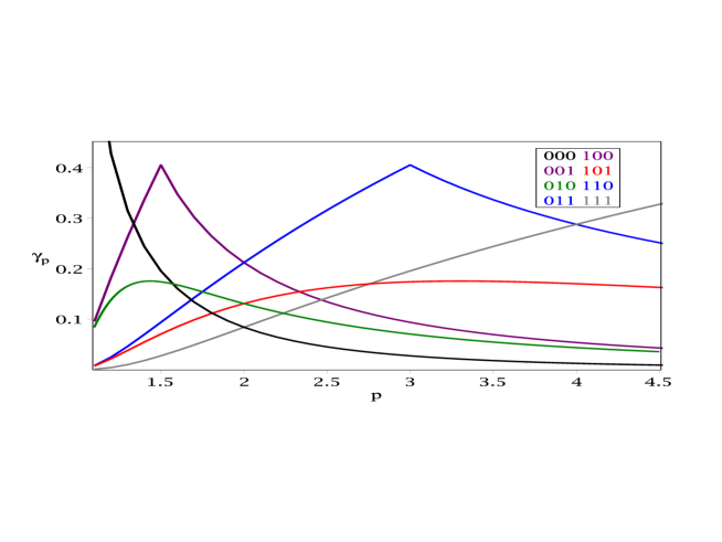
Figure 1: (Colour online) Escape rates for cylinders of length three in the full shift on two symbols $1,0$ with bias $p$. From $p=3$ vertically we have $000,010,001=100,101,111$ and $011=110$.

4 Small hole asymptotics

An additional strength of (6) is that it allows us to study the asymptotic behavior of the escape rate as $\mu_{B}$ shrinks to zero around a given point. Consider a periodic point $x\in X$ of prime period $p$ (the aperiodic case corresponds to $p\rightarrow\infty$). Pick a sequence of shrinking holes defined by words $B_{m}$ chosen to be $m$ concatenated copies of a word $w=w_{1}w_{2}...w_{p}$. The $w_{i}$ correspond to the partition sets $J_{w_{i}}$ visited by the prime periodic orbit of $x$. Denote by $\mu_{w}$ the measure of the interval defined by $w$. The correlation polynomial of each $B_{m}$ is then

$$\phi_{B_{m}}(z)=1+\sum_{n=1}^{m-1}(c_{p}z^{p})^{n}=\frac{1-\mu_{B_{m}}z^{\left|B_{m}\right|}/(\mu_{w}\Lambda_{x})}{1-z^{p}/\Lambda_{x}}$$ (9)

where we use $c_{kp}=c_{p}^{k}$, $\mu_{B_{m}}=c_{p}^{m-1}\mu_{w}$ and define $\Lambda_{x}^{-1}=c_{p}$. For $1D$ maps $\Lambda_{x}$ corresponds to the stability of the prime periodic orbit of $x$. In order to investigate the asymptotic behavior around $\mu_{B}=\epsilon\ll 1$ we rewrite the smallest zero $z_{0}$ of (6) in terms of a formal expansion

$$z_{0}=1+\sum_{k=1}^{\infty}s_{k}\epsilon^{k}.$$ (10)

Using (9) and (10) in (6) along with the fact that $\zeta^{-1}_{cl}(z)=(1-z)G(z)$ for some polynomial $G(z)$ from the Perron-Frobenius theorem, to first order in $\epsilon$ we have,

$$\zeta^{-1}_{op}(z_{0})\approx\frac{-s_{1}\epsilon G(1)}{(1-\Lambda_{x}^{-1})}+\frac{\epsilon}{\mu_{t}}C(1)_{t,r}=0.$$ (11)

Which gives,

$$s_{1}=\frac{C(1)_{t,r}(1-\Lambda_{x}^{-1})}{\mu_{t}G(1)}.$$ (12)

In order to make sense of (12) we firstly derive an important relationship between the transfer operators of the closed and open systems and the operator

$$T(z)=\mathbf{1}+\sum_{n=1}^{\infty}z^{n}T_{n}$$ (13)

where $T_{n}$ is the return time operator of a set $E$ which is defined by $T_{n}\rho=\mathcal{L}^{n}\chi_{E}\rho$ similar to the operators defined in [40]. From (1) we have formally

$$\mathbf{1}-z\mathcal{L}_{op} = \mathbf{1}-z\mathcal{L}+z\mathcal{L}\chi_{E}$$ (14)

$$= (\mathbf{1}-z\mathcal{L})\left(\mathbf{1}+\sum_{n=1}^{\infty}z^{n}\mathcal{L}^{n}\chi_{E}\right)$$

$$= (\mathbf{1}-z\mathcal{L})T(z).$$

We stress that this relation is generic and not restricted to the Markov setting investigated so far. On the other hand, in the present Markov one, we can show that $\det(T(z))=U(z)$ is the generating function of the probability of return to the hole, while $\det(\mathbf{1}-z\mathcal{L}_{op})=\zeta^{-1}_{op}(z)$ and $\det(\mathbf{1}-z\mathcal{L})=\zeta^{-1}_{cl}(z)$. Finally we obtain

$$U(z)=\frac{\zeta^{-1}_{op}(z)}{\zeta^{-1}_{cl}(z)}.$$ (15)

$U(z)$ is related to the generating function of the probability of first-return $F(z)$ via [29],

$$F(z)=\frac{U(z)-1}{U(z)}.$$ (16)

Using (15) and (16) we explicitly show that the decay rate of the first return time distribution of a set $E$ in a closed system, given by the leading pole of $F(z)$, is equal to the escape rate of the system open on $E$ (given by the leading zero of $\zeta^{-1}_{op}(z)$), a previously heuristically derived result [1]. Furthermore, from Kac’s lemma $F^{\prime}(1)=1/\mu_{B}$ and thus, using (15) in (16) we have

$$\frac{1}{\mu_{t}}=\frac{G(1)}{C(1)_{t,r}},$$ (17)

which implies

$$s_{1}=1-\Lambda_{x}^{-1}.$$ (18)

Note that for $p\rightarrow\infty$ (corresponding to $x$ aperiodic) we have $\Lambda_{x}^{-1}\rightarrow 0$ and $s_{1}=1$ (equivalently choose $B_{m}$ to be aperiodic so that $\phi_{B_{m}}(z)=1$ for every $m$ and the result follows).

The first order expansion (18) is consistent with [11], wherein it is shown to be valid for more general chaotic maps. On the other hand, using (9) and (17) one can derive all orders recursively due to the general form of (6). Of particular note is that for a.e. $x\in X$, corresponding to $x$ aperiodic, we have,

$$s_{2}=\left|B\right|-1-\frac{G^{\prime}(1)}{G(1)}+\frac{C^{\prime}(1)_{t,r}}{C(1)_{t,r}}.$$ (19)

From the Entropy (Shannon-McMillan-Breiman) theorem [41], we have that for $\mu$-a.e. $x\in X$, $\left|B\right|\approx-\ln(\epsilon)/h$ for $\left|B\right|\rightarrow\infty$ where $h$ is the metric entropy. That is, in the expansion of $z_{0}$ an $\epsilon^{2}\ln(\epsilon)$ term appears for all subshifts of finite type for $\mu$-a.e. $x\in X$. The appearance of an $\epsilon^{2}\ln(\epsilon)$ term is derived for the doubling map in [13] along with a heuristic argument for why it should be found in a more general setting, as we have confirmed here for the general case of a subshift of finite type.

5 Conclusions

Having an expression for the dynamical zeta function such as equation (6) has allowed us to analytically derive some properties of the escape rate for a paradigmatic class of dynamical systems. From a mathematical viewpoint, we believe that a formal investigation of the accuracy and convergence properties of the proposed framework within the Ulam approximation scheme, could permit the extension of some of the results to more general nonlinear systems. In this respect, care should be taken as it is known that discretization can introduce ‘fake’ eigenvalues (not related to the dynamics) even for linear hyperbolic toral automorphisms, [42], and similar phenomena could potentially appear in open systems. From a physical viewpoint, we expect that some of the methods introduced could be adapted to approximate open systems in different practical situations, such as open billiards [17]. Moreover, note that the formalism is equally valid in situations where some piecewise constant observable is introduced [14] or where an infinite countable partition is used as in intermittent maps [43]. Finally we stress that the equations (6) and (15) allow us to extend Kac-like relations to higher moments of the probability distribution of first-return time [44]: as an example, for a full shift with $\tilde{\phi}_{B}(z)=0$ we find

$$\left<\tau^{2}\right>=\frac{2}{\mu_{B}^{2}}-\frac{2\left|B\right|-1}{\mu_{B}}.$$ (20)

Similar expressions are obtained in the general case. Extending these results will be the subject of future work.

Furthermore, application of the ideas presented in this work, could help in studying the escape rate in more general dynamical systems.

6 References

References

- [1] E G Altmann, J S E Portela, and T Tél. Leaking chaotic systems. Rev. Mod. Phys., 85:869–918, May 2013.
- [2] A Bovier. Metastability. In Roman Kotecký, editor, Methods of Contemporary Mathematical Statistical Physics, Lecture Notes in Mathematics. Springer Berlin Heidelberg, 2009.
- [3] R Pastor-Satorras and A Vespignani. Epidemic spreading in scale-free networks. Phys. Rev. Lett., 86:3200–3203, Apr 2001.
- [4] L A Bunimovich and C P Dettmann. Peeping at chaos: Nondestructive monitoring of chaotic systems by measuring long-time escape rates. Europhys. Lett., 80(4):40001, 2007.
- [5] G Pianigiani and J Yorke. Expanding maps on sets which are almost invariant: decay and chaos. Trans. Amer. Math. Soc, 252:351–366, 1979.
- [6] L P Kadanoff and C Tang. Escape from strange repellers. P. Natl. Acad. Sci. U.S.A., 81(4):pp. 1276–1279, 1984.
- [7] M F. Demers, P Wright, and L-S Young. Entropy, lyapunov exponents and escape rates in open systems. Ergod. Theor. Dyn. Sys., 32(04):1270–1301, 2012.
- [8] M F Demers and L-S Young. Escape rates and conditionally invariant measures. Nonlinearity, 19(2):377, 2006.
- [9] V Paar and N Pavin. Bursts in average lifetime of transients for chaotic logistic map with a hole. Phys. Rev. E, 55:4112–4115, Apr 1997.
- [10] L A Bunimovich and A Yurchenko. Where to place a hole to achieve a maximal escape rate. Israel J. Math., 182:229–252, 2011.
- [11] G Keller and C Liverani. Rare events, escape rates and quasistationarity: Some exact formulae. J. Stat. Phys., 135:519–534, 2009.
- [12] M F Demers and P Wright. Behaviour of the escape rate function in hyperbolic dynamical systems. Nonlinearity, 25(7):2133, 2012.
- [13] C P Dettmann. Open circle maps: small hole asymptotics. Nonlinearity, 26(1):307, 2013.
- [14] A Ferguson and M Pollicott. Escape rates for gibbs measures. Ergod. Theor. Dyn. Sys., 32(03):961–988, 2012.
- [15] H Faisst and B Eckhardt. Lifetimes of noisy repellors. Phys. Rev. E, 68:026215, Aug 2003.
- [16] E G Altmann and A Endler. Noise-enhanced trapping in chaotic scattering. Phys. Rev. Lett., 105:244102, Dec 2010.
- [17] C P Dettmann. Recent advances in open billiards with some open problems. In E. Zearoulia and J.C. Sprott, editors, Frontiers in the Study of Chaotic Dynamical Systems with Open Problems, World Scientific Series on Nonlinear Science, B, Vol. 16. World Scientific Pub. Co. Inc., 2011.
- [18] M A Kouritzin and H Long. Convergence of markov chain approximations to stochastic reaction-diffusion equations. Ann. Appl. Probab., 12(3):pp. 1039–1070, 2002.
- [19] A Tamir. Applications of Markov Chains in Chemical Engineering. Elsevier Science, 1998.
- [20] P Gates and H Tong. On markov chain modeling to some weather data. J. Appl. Meteor., 15:1145–1151, Sep 1976.
- [21] W Y Tan. Applications of some finite markov chain theories to two locus selfing model with selection. Biometrics, 29(2):pp. 331–346, 1973.
- [22] J A Capitán, J A Cuesta, and J Bascompte. Statistical mechanics of ecosystem assembly. Phys. Rev. Lett., 103:168101, Oct 2009.
- [23] M A Novotny. Monte carlo algorithms with absorbing markov chains: Fast local algorithms for slow dynamics. Phys. Rev. Lett., 74:1–5, Jan 1995.
- [24] G Froyland and K Aihara. Estimating statistics of neuronal dynamics via markov chains. Biol. Cybern., 84:31–40, 2001.
- [25] N T Schmandt and R F Galán. Stochastic-shielding approximation of markov chains and its application to efficiently simulate random ion-channel gating. Phys. Rev. Lett., 109:118101, Sep 2012.
- [26] L Ermann and D L Shepelyansky. Ulam method and fractal weyl law for perron-frobenius operators. Eur. Phys. J. B., 75(3):299–304, 2010.
- [27] G Froyland. Extracting dynamical behavior via markov models. In A. I. Mees, editor, Nonlinear Dynamics and Statistics, pages 281–321. Birkhauser Boston, 2001.
- [28] D Lind. Perturbations of shifts of finite type. SIAM J. on Discrete Math., 2(3):350–365, 1989.
- [29] W Feller. An Introduction to Probability Theory and Its Applications, volume 1. Wiley, January 1968.
- [30] A V Chechkin, R Metzler, V Y Gonchar, J Klafter, and L V Tanatarov. First passage and arrival time densities for lévy flights and the failure of the method of images. J. Phys. A: Math. and Gen., 36(41):L537, 2003.
- [31] G Froyland. Using ulam’s method to calculate entropy and other dynamical invariants. Nonlinearity, 12(1):79, 1999.
- [32] W Bahsoun. Rigorous numerical approximation of escape rates. Nonlinearity, 19(11):2529, 2006.
- [33] C Bose, G Froyland, C González-Tokman, and R Murray. Ulam’s method for Lasota-Yorke maps with holes. ArXiv e-prints 1204.2329, April 2012.
- [34] O Georgiou, C P Dettmann, and E G Altmann. Faster than expected escape for a class of fully chaotic maps. Chaos, 22(4):043115, 2012.
- [35] V S Afraimovich and L A Bunimovich. Which hole is leaking the most: a topological approach to study open systems. Nonlinearity, 23(3):643, 2010.
- [36] L J Guibas and A M Odlyzko. Maximal prefix-synchronized codes. SIAM J. Appl. Math., 35(2):pp. 401–418, 1978.
- [37] L J Guibas and A M Odlyzko. Periods in strings. J. Comb. Theory A, 30(1):19 – 42, 1981.
- [38] P. Cvitanović, R Artuso, R Mainieri, G Tanner, and G Vattay. Chaos: Classical and Quantum. Niels Bohr Institute, Copenhagen, 2010. ChaosBook.org.
- [39] G Cristadoro. Fractal diffusion coefficient from dynamical zeta functions. J. Phys. A: Math. and Gen., 39(10):L151, 2006.
- [40] O Sarig. Subexponential decay of correlations. Invent. Math., 150:629–653, 2002.
- [41] P C Shields. Graduate Studies in Mathematics, volume 13. Amer Mathematical Society, 1996.
- [42] M Blank, G Keller, and C Liverani. Ruelle-Perron-Frobenius spectrum for Anosov maps. Nonlinearity, 15(6):1905, 2002.
- [43] P Gaspard and X-J Wang. Sporadicity: Between periodic and chaotic dynamical behaviors. P. Natl. Acad. Sci. U.S.A., 85(13):4591–4595, 1988.
- [44] N Hadyn, J Luevano, G Mantica, and S Vaienti. Multifractal properties of return time statistics. Phys. Rev. Lett., 88:224502, May 2002.