From a complex scalar field to the two-fluid picture of superfluidity

Abstract

The hydrodynamic description of a superfluid is usually based on a two-fluid picture. We compute the basic properties of the relativistic two-fluid system from the underlying microscopic physics of a relativistic $\varphi^{4}$ complex scalar field theory. We work at nonzero but small temperature and weak coupling, and we neglect dissipation. We clarify the relationship between different formulations of the two-fluid model, and how they are parameterized in terms of partly redundant current and momentum 4-vectors. As an application, we compute the velocities of first and second sound at small temperatures and in the presence of a superflow. While our results are of a very general nature, we also comment on their interpretation as a step towards the hydrodynamics of the color-flavor locked state of quark matter, which, in particular in the presence of kaon condensation, appears to be a complicated multi-component fluid.

I Introduction

A superfluid at finite temperature can be described “macroscopically” in terms of a two-fluid model involving a superfluid and a normal fluid. It can also be described “microscopically” in terms of a condensate associated with the spontaneous breaking of a $U(1)$ global symmetry in an underlying field theory. In this paper, we show how to relate the macroscopic hydrodynamics of a non-dissipative relativistic superfluid to the microscopic field-theoretic description.

I.1 Macroscopic two-fluid description

The two-fluid picture was suggested by Tisza Tisza (1938) shortly after the superfluid nature of ⁴He was established experimentally Kapitza (1938); Allen and Misener (1938). At zero temperature, there is only a superfluid component, while at nonzero temperatures below the critical temperature, both fluid components coexist. Landau Landau (1941) predicted a “second sound” mode where the relative densities of the two fluids oscillate, resulting in a temperature (or entropy) wave. This is in contrast to an ordinary sound wave, where the total density (or pressure) oscillates.

The generalization to relativistic superfluids was introduced by Lebedev and Khalatnikov Khalatnikov and Lebedev (1982); Lebedev and Khalatnikov (1982) and Carter Carter (1989). The approaches in these works—termed “potential” and “convective” variational approaches, respectively—differ in their formulation but are equivalent and can be translated into each other Carter and Khalatnikov (1992); Andersson and Comer (2005). The convective approach uses two four-currents, corresponding to total conserved charge and entropy (which is also conserved in the dissipationless case). The potential approach uses two conjugate four-momenta, which correspond to the superfluid four-velocity (multiplied by the chemical potential) and a thermal four-vector whose temporal component is the temperature. The conventional presentation of the two-fluid model, although it looks like two currents (super current and normal current) is really based on one current (the entropy current) and one momentum (proportional to the superfluid velocity). We explain how the various formalisms are related via Legendre transforms of two Lorentz scalar quantities, a generalized pressure and a generalized energy density. We calculate all these quantities in terms of the microscopic theory.

I.2 Microscopic field-theoretic description

The main physical ingredient of a superfluid is a Bose-Einstein condensate, which is responsible for the frictionless flow. This was realized by London, who pointed out the connection between the phenomenology of ⁴He and the quantum statistics of bosons London (1938). In a more modern, field-theoretic language, the superfluid state spontaneously breaks a $U(1)$ symmetry of the underlying Lagrangian. As a consequence, there is a Goldstone mode whose dispersion is linear for small momenta. Using the terminology introduced in the context of ⁴He, this mode is called a phonon. Roughly speaking, thermal excitations of this mode constitute the normal component in the two-fluid picture, while the superfluid component corresponds to the quantum mechanical ground state. We will clarify this distinction below (see Sec. II.2).

Our microscopic model will be a relativistic $\varphi^{4}$ field theory with a $U(1)$ symmetry that is spontaneously broken by a Bose-Einstein condensate of the fundamental scalars. We derive the two-fluid picture from this model. We express the basic currents and momenta of the two-fluid formalism in terms of field-theoretic quantities, and calculate the effective action at nonzero temperature in the presence of a homogeneous, static superflow.

I.3 Previous work and future applications

Our approach is related to several existing studies in the literature. For instance, in Ref. Carter and Langlois (1995) the two-fluid formalism is connected with a simple statistical approach to the phonon contribution, Ref. Comer and Joynt (2003) connects it with a Walecka model describing nuclear matter in a neutron star, and Ref. Nicolis (2011) makes the connection to a very general effective field theory. In Ref. Son (2002), a hydrodynamic interpretation of a field-theoretic effective action was discussed for zero temperature. For the simplified case of a dissipationless, homogeneous fluid, our study is a generalization of this work to nonzero temperatures. In that reference, also an effective Lagrangian for the phonons is formulated which has been employed to study transport properties of quark matter Manuel et al. (2005); Alford et al. (2007); Manuel and Llanes-Estrada (2007); Mannarelli and Manuel (2008); Alford et al. (2008a); Mannarelli and Manuel (2010).

Our study is very general since we do not have to specify the system for which our “microscopic” theory, the $\varphi^{4}$ model, is an effective description. As a specific application, however, we are ultimately interested in a complete hydrodynamic description of the color-flavor locked (CFL) phase of dense quark matter Alford et al. (1999). The hydrodynamics of dense matter, be it dense nuclear or quark matter, is very important for the understanding of the physics of compact stars. One prominent example that relates the hydrodynamic properties to an observable – in this case the rotation frequency of the star – is the $r$-mode instability Andersson (1998), for recent developments relating the instability to microscopic physics see Refs. Jaikumar et al. (2008); Andersson et al. (2010); Alford et al. (2012a, b). Other examples include pulsar glitches, magnetohydrodynamics, and asteroseismology; see for instance Refs. Epstein (1988); Lee (1995); Langlois et al. (1998); Haskell et al. (2012); Glampedakis et al. (2012) for applications of multi-fluid hydrodynamics in the astrophysical context. Since the densities in the cores of compact stars can be as large as several times nuclear ground state density, it is conceivable that the cores are made of deconfined quark matter. The CFL phase is the ground state of three-flavor, asymptotically dense quark matter and therefore also of fundamental theoretical interest. Whether it persists down to densities that exist inside a compact star is unknown, and many other candidate phases have been discussed Alford et al. (2008b). Taking into account the effect of a non-negligible strange quark mass, the next phase down in density appears to be the kaon-condensed CFL phase (CFL-$K^{0}$) Bedaque and Schäfer (2002), whose superfluid properties are expected to be nontrivial. Firstly, the quark Cooper pair condensate of CFL spontaneously breaks the $U(1)$ associated with baryon number conservation, making CFL a baryon superfluid. Secondly, the kaon condensate in CFL-$K^{0}$ spontaneously breaks the $U(1)$ associated with strangeness conservation. This $U(1)$, however, is explicitly broken since weak interactions have to be taken into account in the astrophysical context. As a consequence, the corresponding Goldstone mode has a mass of the order of $50\,{\rm keV}$ Son (2001a) which is small compared to the critical temperature for kaon condensation, estimated to be of the order of tens of MeV Alford et al. (2008c). Therefore, the question arises how many (super)fluid components CFL-$K^{0}$ has, and how the two-fluid picture is modified (or whether superfluidity survives in any sense) when there is a small explicit symmetry breaking of the $U(1)$.

I.4 Overview

In Sec. II we start with the zero-temperature case, where the relation between field theory and superfluid hydrodynamics is well established. We elaborate on this relation, which sets the notation and prepares us for the nonzero-temperature case. The remaining paper is divided into four parts: the microscopic nonzero-temperature calculation, Sec. III, introducing the two-fluid formalism, Sec. IV, and connecting both, Sec. V; then we use our results to compute the sound velocities in the presence of a superflow in Sec. VI.

Our convention for the metric tensor is $g^{\mu\nu}={\rm diag}(1,-1,-1,-1)$. Our units are $\hbar=c=k_{B}=1$. We work in the imaginary-time formalism, i.e., $T/V\sum_{k}\equiv T\sum_{n}\int d^{3}{\bf k}/(2\pi)^{3}$, where $n$ labels the Matsubara frequencies $\omega_{n}\equiv ik_{0}$. For bosons $\omega_{n}=2n\pi T$, for fermions $\omega_{n}=(2n+1)\pi T$.

II Zero temperature: single fluid

II.1 Lagrangian

Our starting point is the Lagrangian

$${\cal L}=\partial_{\mu}\varphi\partial^{\mu}\varphi^{*}-m^{2}|\varphi|^{2}-\lambda|\varphi|^{4}\,,$$ (1)

with the complex scalar field $\varphi$, the mass parameter $m>0$, and the coupling constant $\lambda>0$. The Lagrangian is obviously invariant under global $U(1)$ rotations $\varphi\to e^{i\alpha}\varphi$ which leads to a conserved charge. Later, in our explicit low-temperature results, we shall set $m=0$ for simplicity. Note that, since $m^{2}>0$, the quadratic term of the classical potential is positive, and spontaneous symmetry breaking can only occur if we introduce a chemical potential associated to the conserved charge. If this chemical potential is larger than $m$, a Bose-Einstein condensate of the particles is formed. In our formalism, we shall introduce such a chemical potential through the time dependence of the phase of the order parameter.

We allow for Bose-Einstein condensation in the usual way by separating the condensate,

$$\varphi(x)=\frac{e^{i\psi(x)}}{\sqrt{2}}\left[\rho(x)+\varphi^{\prime}_{1}(x)+i\varphi^{\prime}_{2}(x)\right]\,.$$ (2)

Here, $\rho(x)$ is the modulus and $\psi(x)$ the phase of the condensate. For convenience, we have introduced the transformed fluctuation field $\varphi^{\prime}(x)$, which we have written in terms of its real and imaginary parts. Inserting this into the Lagrangian yields

$${\cal L}=-U+{\cal L}^{(1)}+{\cal L}^{(2)}+{\cal L}^{(3)}+{\cal L}^{(4)}\,,$$ (3)

with the tree-level potential

$$U=-\frac{1}{2}\partial_{\mu}\rho\,\partial^{\mu}\rho-\frac{\rho^{2}}{2}(\partial_{\mu}\psi\partial^{\mu}\psi-m^{2})+\frac{\lambda}{4}\rho^{4}\,,$$ (4)

and the fluctuation terms, listed by their order in the fluctuation from linear to quartic,

$${\cal L}^{(1)} = \partial_{\mu}\psi(\rho\partial^{\mu}\varphi_{2}^{\prime}-\varphi_{2}^{\prime}\partial^{\mu}\rho)+\rho(\partial_{\mu}\psi\partial^{\mu}\psi-m^{2}-\lambda\rho^{2})\varphi_{1}^{\prime}+\partial_{\mu}\varphi_{1}^{\prime}\partial^{\mu}\rho\,,$$ (5a)

$${\cal L}^{(2)} = \frac{1}{2}\Big{[}\partial_{\mu}\varphi_{1}^{\prime}\partial^{\mu}\varphi_{1}^{\prime}+\partial_{\mu}\varphi_{2}^{\prime}\partial^{\mu}\varphi_{2}^{\prime}+(\varphi_{1}^{\prime 2}+\varphi_{2}^{\prime 2})(\partial_{\mu}\psi\partial^{\mu}\psi-m^{2})$$ (5b)

$$+\,2\partial_{\mu}\psi(\varphi_{1}^{\prime}\partial^{\mu}\varphi_{2}^{\prime}-\varphi_{2}^{\prime}\partial^{\mu}\varphi_{1}^{\prime})-\lambda\rho^{2}(3\varphi_{1}^{\prime 2}+\varphi_{2}^{\prime 2})\Big{]}\,,$$

$${\cal L}^{(3)} = -\lambda\rho\varphi_{1}^{\prime}(\varphi_{1}^{\prime 2}+\varphi_{2}^{\prime 2})\,,$$ (5c)

$${\cal L}^{(4)} = -\frac{\lambda}{4}(\varphi_{1}^{\prime 2}+\varphi_{2}^{\prime 2})^{2}\,.$$ (5d)

In this paper, we shall only need the tree-level potential and the terms quadratic in the fluctuations. We neglect the cubic and quartic terms because we restrict ourselves to the one-loop effective action, see discussion at the beginning of Sec. III. The linear terms ${\cal L}^{(1)}$ can be rewritten such that they are – up to a total derivative term – proportional to the equations of motion (6), and thus they do not contribute to the on-shell action.

II.2 Zero-temperature hydrodynamics

Let us first discuss the tree-level potential and ignore all fluctuations. This allows us to present the translation to the hydrodynamic equations and quantities in the simplest case, based on Ref. Son (2002). Later we shall include fluctuations to generalize this translation to nonzero temperatures.

The classical equations of motion are

$$\Box\rho = \rho(\sigma^{2}-m^{2}-\lambda\rho^{2})\,,$$ (6a)

$$\partial_{\mu}(\rho^{2}\partial^{\mu}\psi) = 0\,,$$ (6b)

where we have abbreviated

$$\sigma^{2}\equiv\partial_{\mu}\psi\partial^{\mu}\psi\,.$$ (7)

The field-theoretic expressions for the conserved charge current and the stress-energy tensor are

$$j^{\mu} = \frac{\partial{\cal L}}{\partial(\partial_{\mu}\psi)}=\rho^{2}\partial^{\mu}\psi\,,$$ (8a)

$$T^{\mu\nu} = \frac{2}{\sqrt{-g}}\frac{\delta(\sqrt{-g}\,{\cal L})}{\delta g_{\mu\nu}}=2\frac{\partial{\cal L}}{\partial g_{\mu\nu}}-g^{\mu\nu}{\cal L}=\partial^{\mu}\rho\,\partial^{\nu}\rho+\rho^{2}\partial^{\mu}\psi\partial^{\nu}\psi-g^{\mu\nu}{\cal L}\,,$$ (8b)

For the stress-energy tensor, we have used the gravitational definition by formally introducing a general metric $g$ which, after taking the derivatives, we set to be the metric of flat Minkowski space. This definition guarantees that $T^{\mu\nu}$ is symmetric and conserved. Since $j^{\mu}$ is also conserved, we have

$$\partial_{\mu}j^{\mu}=0\,,\qquad\partial_{\mu}T^{\mu\nu}=0\,,$$ (9)

which are the hydrodynamic equations. As we expect from Noether’s theorem, current conservation is identical to the equation of motion (6b) for $\psi$.

As an ansatz for the solution of the equations of motion we may choose

$$\psi = p_{\mu}x^{\mu}+{\rm Re}\sum_{\bf k}\delta\psi_{\bf k}\,e^{i(\omega t-{\bf k}\cdot{\bf x})}\,,$$ (10a)

$$\rho = \sqrt{\frac{p^{2}-m^{2}}{\lambda}}+{\rm Re}\sum_{\bf k}\delta\rho_{\bf k}\,e^{i(\omega t-{\bf k}\cdot{\bf x})}\,.$$ (10b)

In this ansatz, we assume $\partial^{\mu}\psi$ and $\rho$ are each composed of a static part plus small oscillations around it. The static part of the solution is the superfluid mode, corresponding to an infinite and uniformly flowing superfluid. The density and flow are specified by the values of the components of $p_{\mu}$, which are pure numbers, not functions of $x$, and are not constrained by the equation of motion. The value of $p_{\mu}$ is determined by the boundary conditions, which specify the topology of the field configuration, namely the number of times the phase winds around as we traverse the space-time region in which the superfluid resides. The oscillations around the static solution yield two modes whose dispersion relations $\omega({\bf k})$ are determined by the equations of motion. One of the modes is the massless Goldstone mode, the other is a massive “radial” mode. The oscillatory modes can be thermally populated to yield the normal fluid. The boundary conditions place no constraint on the amplitudes of the oscillatory modes because they are topologically trivial.

In this section we will assume uniform density and flow of the superfluid, but in general one could obtain a space-time-dependent superfluid flow by giving nonzero classical background values to the $\delta\psi_{\bf k}$ and $\delta\rho_{\bf k}$. The normal fluid would then consist of a thermal population on top of that background.

In Sec. III.1 we will use the poles of the tree-level propagator to determine the dispersion relation of the oscillatory modes. This yields the same result as solving the equations of motion (6) with the ansatz (10). Oscillations in $\psi$ will also be relevant to the calculation of the sound velocities in Sec. VI. In fact, the coefficient of the linear term in the massless mode $\omega({\bf k})$ is nothing but the velocity of first sound. For now, we set $\delta\psi_{\bf k}=\delta\rho_{\bf k}=0$. In this case, $p^{\mu}=\partial^{\mu}\psi$, and we can write

$$\rho=\sqrt{\frac{\sigma^{2}-m^{2}}{\lambda}}\,.$$ (11)

Inserting this solution back into the Lagrangian gives

$${\cal L}=-U=\frac{(\sigma^{2}-m^{2})^{2}}{4\lambda}\,.$$ (12)

It is clear from the usual definition of the pressure in terms of the partition function that, in our current tree-level treatment, this Lagrangian is identical to the pressure.

We now explore the connection between field-theoretic quantities and hydrodynamics. The hydrodynamic approach involves writing the current and stress-energy tensor in terms of fluid-mechanical quantities

$$j^{\mu} = n_{s}v^{\mu}\,,$$ (13a)

$$T^{\mu\nu} = (\epsilon_{s}+P_{s})v^{\mu}v^{\nu}-g^{\mu\nu}P_{s}\,,$$ (13b)

where $v^{\mu}$ is the superfluid velocity; by definition $v_{\mu}v^{\mu}=1$. To identify $n_{s}$, $\epsilon_{s}$, and $P_{s}$ we go to the superfluid rest frame $v^{\mu}=(1,0,0,0)$, where there is no flow of charge, energy, or momentum: $j^{i}=T^{0i}=0$. Then we have $j^{0}=n_{s}$, $T^{00}=\epsilon_{s}$, $T^{ij}=\delta^{ij}P_{s}$, so $n_{s}$, $\epsilon_{s}$, and $P_{s}$ are the charge density, energy density, and pressure in the superfluid rest frame; the pressure is isotropic. (We will discuss the superfluid density $\rho_{s}$ below). They can be expressed covariantly via appropriate contractions,

$$n_{s}=\sqrt{j^{\mu}j_{\mu}}=v^{\mu}j_{\mu}\,,\qquad\epsilon_{s}=v_{\mu}v_{\nu}T^{\mu\nu}\,,\qquad P_{s}=-\frac{1}{3}(g_{\mu\nu}-v_{\mu}v_{\nu})T^{\mu\nu}\,.$$ (14)

To relate these hydrodynamical quantities to the microscopic physics we can use Eqs. (8). For $n_{s}$ and $v^{\mu}$ we obtain immediately from (8a),

$$n_{s}=\sigma\frac{\sigma^{2}-m^{2}}{\lambda}\,,\qquad v^{\mu}=\frac{\partial^{\mu}\psi}{\sigma}=\gamma\,(1,{\bf v}_{s})\ ,$$ (15)

where ${\bf v}_{s}$ is the superfluid 3-velocity with Lorentz factor $\gamma=1/\sqrt{1-{\bf v}_{s}^{2}}$. The velocity is proportional to the gradient of a scalar field, ${\bf v}_{s}=-\nabla\psi/\partial_{0}\psi$, which is what one expects since a superfluid without vortices is irrotational. [The minus sign appears because the 3-velocity ${\bf v}_{s}$ corresponds to the spatial components of the contravariant 4-vector $v^{\mu}$, while the operator $\nabla$ corresponds to the spatial components of the covariant 4-vector $\partial_{\mu}$, i.e., $\partial^{\mu}=(\partial_{t},-\nabla)$.]

For $\epsilon_{s}$ and $P_{s}$ we first use (14) and (8b) to obtain partly microscopic expressions

$$\epsilon_{s} = v_{\mu}\partial^{\mu}\psi\,n_{s}-{\cal L}\,,\qquad P_{s}={\cal L}+(v_{\mu}\partial^{\mu}\psi-\sigma)n_{s}\,.$$ (16)

From contracting the relation for $v^{\mu}$ in (15) with $\partial_{\mu}\psi$ we know that $v^{\mu}\partial_{\mu}\psi=\sigma$; as a consequence, we obtain the expected relation $P_{s}={\cal L}$. We can now identify the physical meaning of $\sigma$: using the zero-temperature thermodynamic relation in the superfluid rest frame $\epsilon_{s}+P_{s}=\mu_{s}n_{s}$, we find

$$\mu_{s}=\sigma=v^{\mu}\partial_{\mu}\psi\,,$$ (17)

so $\sigma$ is identified with $\mu_{s}$, the chemical potential in the superfluid rest frame. Going back to the solution for the modulus of the condensate (11) we see that, as expected, Bose condensation only occurs for $\mu_{s}^{2}>m^{2}$. Using (12) and (16) we finally obtain fully microscopic expressions for the energy density and the pressure,

$$P_{s}=\frac{(\sigma^{2}-m^{2})^{2}}{4\lambda}\,,\qquad\epsilon_{s}=\frac{(3\sigma^{2}+m^{2})(\sigma^{2}-m^{2})}{4\lambda}\,.$$ (18)

Note that $m$ is the only mass scale in our Lagrangian. The trace of the stress-energy tensor $T^{\mu}{}_{\mu}=\epsilon_{s}-3P_{s}=m^{2}\rho^{2}$ vanishes for $m=0$.

Finally, the superfluid density $\rho_{s}$ is defined via the expansion in small three-velocities of the momentum and energy densities

$$T^{0i}=\rho_{s}{\bf v}_{si}+{\cal O}(|{\bf v}_{s}|^{3})\,,\qquad T^{00}=\frac{\epsilon_{s}+P_{s}{\bf v}_{s}^{2}}{1-{\bf v}_{s}^{2}}=\epsilon_{s}+\rho_{s}{\bf v}_{s}^{2}+{\cal O}(|{\bf v}_{s}|^{4})\,.$$ (19)

From these expansions we obtain its microscopic form

$$\rho_{s}=\epsilon_{s}+P_{s}=\sigma^{2}\frac{\sigma^{2}-m^{2}}{\lambda}\,.$$ (20)

II.3 Single-fluid formalism

Let us now, following Refs. Khalatnikov and Lebedev (1982); Lebedev and Khalatnikov (1982); Carter (1989); Carter and Khalatnikov (1992); Andersson and Comer (2005), introduce the formalism that we shall use below to describe the two fluid components at nonzero temperature. Although this might seem unnecessary for the zero-temperature case where there is only a single fluid, it is a useful preparation for the nonzero temperature case.

In the hydrodynamic formalism, the basic variables that describe one fluid are $j^{\mu}$, which is the conserved current density, and $\partial^{\mu}\psi$, which we will identify as the conjugate momentum. Motivated by Eqs. (8), we write the stress-energy tensor as a function of these variables

$$T^{\mu\nu}=-g^{\mu\nu}\Psi+j^{\mu}\partial^{\nu}\psi\,,$$ (21)

where we call $\Psi$ the generalized pressure, and we define the generalized energy density

$$\Lambda\equiv T^{\mu}_{\;\;\mu}+3\Psi=-\Psi+j^{\mu}\partial_{\mu}\psi\,.$$ (22)

By comparison with the expressions from the previous subsection it is easy to see that in the single-fluid case $\Psi$ and $\Lambda$ are simply pressure and energy density in the fluid rest frame, $\Psi=P_{s}={\cal L}$, $\Lambda=\epsilon_{s}$. It is then natural to treat $\Lambda$ and $\Psi$ as Legendre transforms of each other: $\Psi$ depends only on $\partial^{\mu}\psi$, and we assume that $\Lambda$ depends only on $j^{\mu}$ (the fact that $\partial\Lambda/\partial(\partial_{\mu}\psi)=0$ follows from (22) and (8a)). So

$$d\Lambda=\partial_{\mu}\psi\,dj^{\mu}\,,\qquad d\Psi=j^{\mu}d(\partial_{\mu}\psi)\,.$$ (23)

Since $\Lambda$ and $\Psi$ are Lorentz scalars, they depend on the Lorentz scalars $j^{2}=j_{\mu}j^{\mu}=n_{s}^{2}$ and $\sigma^{2}=\partial_{\mu}\psi\partial^{\mu}\psi$, respectively. This allows us to write

$$\partial_{\mu}\psi=\frac{\partial\Lambda}{\partial j^{\mu}}={\cal B}\,j_{\mu}\,,\qquad{\cal B}\equiv 2\frac{\partial\Lambda}{\partial j^{2}}\,,$$ (24)

and

$$j^{\mu}=\frac{\partial\Psi}{\partial(\partial_{\mu}\psi)}=\overline{\cal B}\,\partial^{\mu}\psi\,,\qquad\overline{\cal B}\equiv 2\frac{\partial\Psi}{\partial\sigma^{2}}\,.$$ (25)

These relations say that the current is proportional to the conjugate momentum with a coefficient given by the underlying microscopic physics. In this one-fluid system, we simply read off

$$\overline{\cal B}={\cal B}^{-1}=\frac{\sigma^{2}-m^{2}}{\lambda}\,.$$ (26)

This formalism will allows us to introduce the so-called entrainment coefficients as the coefficients in a two-fluid system which relate the current of the first fluid with the conjugate momentum of the second fluid and vice versa. But before we do so, we go back to our microscopic calculation to “prepare” it for the translation into the two-fluid picture.

III Nonzero temperature: microscopic calculation

III.1 Effective action and anisotropic dispersions

In our context, the nonzero-temperature calculation is complicated for two reasons: $(i)$ we are interested in the situation of a nonzero (homogeneous) superflow; this makes the system and in particular the dispersions of the Goldstone mode anisotropic and $(ii)$ in order to compute the properties of the system for all temperatures up to the critical temperature, a self-consistent formalism such as the Cornwall-Jackiw-Tomboulis (CJT) formalism Luttinger and Ward (1960); Baym (1962); Cornwall et al. (1974) is needed. (For a detailed discussion of this formalism in the same context, but without superflow, see Ref. Alford et al. (2008c).)

Here we are mostly interested in analytical results to discuss the translation to hydrodynamics thoroughly. Therefore, we shall restrict ourselves to small temperatures and ignore the complications from point $(ii)$. This means that we shall not determine the condensate self-consistently, and rather work with its zero-temperature value. Starting from the full self-consistent formalism, one can show that the temperature-dependence of the condensate includes an additional power of the coupling constant compared to the terms we are keeping. We are thus working in the low-temperature, weak-coupling approximation. Note, however, that the melting of the condensate, as well as other contributions from the full action may induce terms proportional to $\lambda\mu^{2}T^{2}$ in the pressure, while we shall only keep terms proportional to $T^{4}$ and higher order in $T$. This approximation is only consistent if $T^{2}\gg\lambda\mu^{2}$, i.e., strictly speaking, our approximation leaves a “gap” between $T=0$ and the small temperatures we are discussing, although this gap can be made arbitrarily small by choosing the coupling constant $\lambda$ sufficiently small. We defer a careful discussion of the self-consistent CJT calculation with superflow, including a numerical evaluation up to the critical temperature to a forthcoming publication Alford et al. (in preparation).

Within this approximation, we can work with the simple one-loop effective action

$$\Gamma=-\frac{V}{T}\,U(\rho,\sigma)-\frac{1}{2}\sum_{k}{\rm Tr}\ln\frac{S^{-1}(k)}{T^{2}}\,,$$ (27)

with the tree-level potential $U$ from Eq. (4) and the inverse tree-level propagator in momentum space $S^{-1}(k)$ which can be read off from the terms quadratic in the fluctuations in Eq. (5b). The trace is taken over the $2\times 2$ space of the two real degrees of freedom of the complex scalar field, and the sum is taken over four-momenta $k_{\mu}=(k_{0},{\bf k})$, $k_{0}=-i\omega_{n}$ with the bosonic Matsubara frequencies $\omega_{n}$. The sum over three-momenta, here written for a finite volume $V$ and thus over discrete momenta, becomes an integral in the thermodynamic limit. At the stationary point, i.e., with Eq. (11), we have

$$S^{-1}(k)=\left(\begin{array}[]{cc}-k^{2}+2(\sigma^{2}-m^{2})&2ik\cdot\partial\psi\\[8.61108pt] -2ik\cdot\partial\psi&-k^{2}\end{array}\right)\,.$$ (28)

Here, $k^{2}\equiv k_{\mu}k^{\mu}$, $k\cdot\partial\psi=k_{\mu}\partial^{\mu}\psi$ and $\sigma$ given in Eq. (7). In all our microscopic calculations we evaluate thermal fluctuations in the background of a uniform superflow, so we take $\partial_{\mu}\psi$ (and hence $\sigma$) to be space-time independent. Since we neglect the melting of the condensate, we have inserted the zero-temperature solution into the propagator.

In order to compute the effective action, one may employ partial integration with respect to the $|{\bf k}|$ integral. The effective action density then becomes

$$\frac{T}{V}\Gamma = \frac{(\sigma^{2}-m^{2})^{2}}{4\lambda}-\frac{2}{3}\frac{T}{V}\sum_{k}\frac{{\bf k}^{2}(k^{2}-\sigma^{2}+m^{2})+2k\cdot\partial\psi\,{\bf k}\cdot\nabla\psi}{{\rm det}\,S^{-1}(k)}\,,$$ (29)

where we have used the explicit form of the tree-level propagator and have performed the $2\times 2$ trace. We have also inserted the solution (11) into the potential $U$. The evaluation of the Matsubara sum and the simplification of the result is explained in detail in appendix A. Neglecting the thermal contribution of the massive mode, we can write the result as

$$\frac{T}{V}\Gamma \simeq \frac{(\sigma^{2}-m^{2})^{2}}{4\lambda}-\int\frac{d^{3}{\bf k}}{(2\pi)^{3}}\frac{F(\epsilon_{1,{\bf k}},{\bf k})}{(\epsilon_{1,{\bf k}}+\epsilon_{1,-{\bf k}})(\epsilon_{1,{\bf k}}+\epsilon_{2,-{\bf k}})(\epsilon_{1,{\bf k}}-\epsilon_{2,{\bf k}})}\,\coth\frac{\epsilon_{1,{\bf k}}}{2T}\,,$$ (30)

where $F(k_{0},{\bf k})$ denotes the numerator in the momentum sum of Eq. (29),

$$F(k_{0},{\bf k})\equiv-\frac{2}{3}\left[{\bf k}^{2}(k^{2}-\sigma^{2}+m^{2})+2k\cdot\partial\psi\,{\bf k}\cdot\nabla\psi\right]\,,$$ (31)

and where $\epsilon_{1/2,{\bf k}}$ are complicated excitation energies whose small-momentum approximations are

$$\epsilon_{1,{\bf k}} = \sqrt{\frac{\sigma^{2}-m^{2}}{3\sigma^{2}-m^{2}}}\;\zeta(\hat{\mathbf{k}})\,|{\bf k}|+{\cal O}(|{\bf k}|^{3})\,,$$ (32a)

$$\epsilon_{2,{\bf k}} = \sqrt{2}\sqrt{3\sigma^{2}-m^{2}+2(\nabla\psi)^{2}}+{\cal O}(|{\bf k}|)\,.$$ (32b)

Here we have abbreviated

$$\zeta(\hat{\mathbf{k}})\equiv\left[\sqrt{1+2\frac{(\nabla\psi)^{2}-(\nabla\psi\cdot\hat{\mathbf{k}})^{2}}{3\sigma^{2}-m^{2}}}-\frac{2\partial_{0}\psi\nabla\psi\cdot\hat{\mathbf{k}}}{\sqrt{\sigma^{2}-m^{2}}\sqrt{3\sigma^{2}-m^{2}}}\right]\left[1+\frac{2(\nabla\psi)^{2}}{3\sigma^{2}-m^{2}}\right]^{-1}\,.$$ (33)

The physically relevant low-energy excitation is $\epsilon_{1,{\bf k}}$. This is the Goldstone mode which, as Eq. (32a) confirms, is massless and linear in the momentum for small momenta, as it should be. The coefficient in front of the linear term is the speed of (first) sound. For the case without superflow we have $\zeta(\hat{\mathbf{k}})=1$, and thus, in the limit $m=0$, we recover the well-known $1/\sqrt{3}$. The superflow introduces an angular dependence $\zeta(\hat{\mathbf{k}})$ into the Goldstone dispersion and thus also into the sound velocity. This angular-dependent function also shows that, in contrast to the zero-temperature case, we cannot write the result in a covariant way since the temporal and spatial components of $\partial_{\mu}\psi$ appear separately. Another observation is the complicated factor in the integrand of Eq. (30). This factor indicates a mixing between the original modes of the complex field (between particles and antiparticles, essentially) due to condensation. Such a factor appears also, although considerably simpler, for the case without superflow. It is analogous to a Bogoliubov coefficient in the case of Cooper pairing which, in that case, accounts for the mixing between fermions and fermion-holes.

We shall further evaluate the effective action for small temperatures in Sec. III.3.

III.2 Stress-energy tensor and current

The stress-energy tensor and the current are given by

$$T^{\mu\nu}=\left\langle\frac{2}{\sqrt{-g}}\frac{\delta(\sqrt{-g}\,{\cal L})}{\delta g_{\mu\nu}}\right\rangle\,,\qquad j^{\mu}=\left\langle\frac{\partial{\cal L}}{\partial(\partial_{\mu}\psi)}\right\rangle\,,$$ (34)

where the angular brackets denote the expectation value in the finite-temperature ensemble of the microscopic theory,

$$\langle A\rangle\equiv\frac{1}{Z}\int{\cal D}\varphi_{1}^{\prime}{\cal D}\varphi_{2}^{\prime}\,A\,\exp\left(\int d^{4}x\,{\sqrt{-g}\,{\cal L}}\right)\,,$$ (35)

with the partition function $Z$ defined so that $\langle 1\rangle=1$. After performing the functional integral we can write the results as

$$T^{\mu\nu} = -\left(2\frac{\partial U}{\partial g_{\mu\nu}}-g^{\mu\nu}U\right)-\frac{T}{V}\sum_{k}{\rm Tr}\left[S(k)\frac{\partial S^{-1}(k)}{\partial g_{\mu\nu}}-\frac{g^{\mu\nu}}{2}\right]\,,$$ (36a)

$$j^{\mu} = \partial^{\mu}\psi\,\frac{\sigma^{2}-m^{2}}{\lambda}-\frac{1}{2}\frac{T}{V}\sum_{k}{\rm Tr}\left[S(k)\frac{\partial S^{-1}(k)}{\partial(\partial_{\mu}\psi)}\right]\,.$$ (36b)

In the case of the stress-energy tensor, one can check explicitly that the sum over the Matsubara frequencies leads to an infinite result. A renormalization is thus required. As a renormalization condition, we require for the case without superflow the obvious interpretation of the diagonal components $T^{\mu\nu}$ in terms of the energy density $\epsilon$ and the pressure $P$,

$$T^{00}=\epsilon\,,\qquad T^{ij}=\delta^{ij}P\,.$$ (37)

Then, switching on a nonzero superflow, does not yield any additional divergences. These conditions can be implemented on a very general level, without explicit evaluation of the stress-energy tensor. We do so in detail in appendix B. The calculation in this appendix also leads to a very useful formulation of the effective action, the stress-energy tensor, and the current, which will later facilitate the interpretation in terms of the hydrodynamic two-fluid picture. We define (for motivation see Eq. (72))

$$\Psi_{k}\equiv\Psi_{k}(\sigma^{2},k\cdot\partial\psi,k^{2})\equiv-\frac{1}{2}{\rm Tr}\ln\frac{S^{-1}(k)}{T^{2}}\,,$$ (38)

and

$$A_{k} \equiv \frac{\partial\Psi_{k}}{\partial(k\cdot\partial\psi)}=4\frac{k\cdot\partial\psi}{{\rm det}\,S^{-1}}\,,$$ (39a)

$$B_{k} \equiv 2\frac{\partial\Psi_{k}}{\partial\sigma^{2}}=\frac{2k^{2}}{{\rm det}\,S^{-1}}\,,$$ (39b)

$$C_{k} \equiv 2\frac{\partial\Psi_{k}}{\partial k^{2}}=-\frac{2(k^{2}-\sigma^{2}+m^{2})}{{\rm det}\,S^{-1}}\,.$$ (39c)

The reason to introduce these quantities and the choice of notation will become clear after we have discussed the two-fluid formalism. In the zero-temperature discussion of the single-fluid dynamics we have already encountered the generalized pressure $\Psi$, of which the notation $\Psi_{k}$ is reminiscent. The notations $A_{k}$, $B_{k}$, $C_{k}$ are chosen in analogy to $\overline{\cal A}$, $\overline{\cal B}$, $\overline{\cal C}$, to be introduced in Sec. IV.1 (we already know the coefficient $\overline{\cal B}$ from the single-fluid treatment in Sec. II.3). With the help of these quantities we can write the action as (see appendix B)

$$\frac{T}{V}\Gamma=-U-\frac{1}{3}(g^{\mu\nu}-u^{\mu}u^{\nu})\frac{T}{V}\sum_{k}\left(C_{k}k_{\mu}k_{\nu}+A_{k}k_{\mu}\partial_{\nu}\psi\right)\,,$$ (40)

where we have abbreviated $u^{\mu}=(1,0,0,0)$, while the renormalized stress-energy tensor and the current become

$$T^{\mu\nu} = -\left(2\frac{\partial U}{\partial g_{\mu\nu}}-g^{\mu\nu}U\right)+\frac{T}{V}\sum_{k}\left[C_{k}k^{\mu}k^{\nu}+B_{k}\partial^{\mu}\psi\partial^{\nu}\psi+A_{k}(k^{\mu}\partial^{\nu}\psi+k^{\nu}\partial^{\mu}\psi)+2u^{\mu}u^{\nu}\right]\,,$$ (41a)

$$j^{\mu} = \partial^{\mu}\psi\,\frac{\sigma^{2}-m^{2}}{\lambda}+\frac{T}{V}\sum_{k}\left(B_{k}\partial^{\mu}\psi+A_{k}k^{\mu}\right)\,.$$ (41b)

It is instructive to compute the trace of the stress-energy tensor. With the help of Eq. (94) we immediately find

$$T^{\mu}_{\;\;\mu}=m^{2}\left[\rho^{2}+2\frac{T}{V}\sum_{k}\frac{k^{2}}{{\rm det}\,S^{-1}(k)}\right]\,,$$ (42)

i.e., the trace vanishes when we set $m=0$, as expected.

III.3 Evaluation for small temperatures

We want to compute the effective action, the components of the stress-energy tensor, and the current for small temperatures explicitly. To this end, we have to approximate momentum sums of the form

$$\frac{T}{V}\sum_{k}\frac{F(k)}{{\rm det}\,S^{-1}(k)}\,,$$ (43)

where, for the case of the effective action, $F(k)$ is given by Eq. (31), and for the stress-energy tensor and the current we need to replace $F(k)$ by

$$F^{\mu\nu}(k) \equiv 2\left[-(k^{2}-\sigma^{2}+m^{2})k^{\mu}k^{\nu}+k^{2}\partial^{\mu}\psi\partial^{\nu}\psi+2(k\cdot\partial\psi)(k^{\mu}\partial^{\nu}\psi+k^{\nu}\partial^{\mu}\psi)+u^{\mu}u^{\nu}{\rm det}\,S^{-1}(k)\right]\,,$$ (44a)

$$F^{\mu}(k) \equiv 2(k^{2}\partial^{\mu}\psi+2k\cdot\partial\psi\,k^{\mu})\,,$$ (44b)

which can be read off from Eqs. (41).

For all three cases, we can write the result of the Matsubara sum in the form (30). Then, we write $\coth[\epsilon_{1,{\bf k}}/(2T)]=1+2f(\epsilon_{1,{\bf k}})$ with the Bose distribution function $f(x)=1/(e^{x/T}-1)$. The integral over the first term is, in our approximation, temperature independent. It is divergent and has to be renormalized by subtracting the vacuum contribution. After doing so, a finite term remains which however is suppressed by one power of $\lambda$ compared to the zero-temperature term $\propto\lambda^{-1}$ we have already computed, for instance in Eq. (30). We shall thus neglect this contribution and only keep the thermal contribution, i.e., the integral over the second term that contains the Bose function. This contribution is finite and unaffected by the renormalization.

We explain the small-temperature expansion in detail in appendix C. Before we come to the main results, let us discuss the simpler example without superflow, $\nabla\psi=0$. In this case, $\epsilon_{1,{\bf k}}=\epsilon_{k}^{+}$, $\epsilon_{2,{\bf k}}=\epsilon_{k}^{-}$ with

$$\epsilon_{k}^{\pm}=\sqrt{k^{2}+3\mu^{2}-m^{2}\mp\sqrt{4\mu^{2}k^{2}+(3\mu^{2}-m^{2})^{2}}}\,,$$ (45)

where we have set $\partial_{0}\psi=\mu$. Here, $\epsilon_{k}^{+}$ is the Goldstone mode, while $\epsilon_{k}^{-}$ is the massive mode. This yields the small-temperature result for the pressure to order $T^{6}$ (see appendix C),

$$P=\frac{T}{V}\Gamma(\nabla\psi=0) \simeq \frac{(\mu^{2}-m^{2})^{2}}{4\lambda}+\frac{(3\mu^{2}-m^{2})^{3/2}}{(\mu^{2}-m^{2})^{3/2}}\frac{\pi^{2}T^{4}}{90}-\frac{\mu^{6}(3\mu^{2}-m^{2})^{1/2}}{(\mu^{2}-m^{2})^{7/2}}\frac{4\pi^{4}T^{6}}{63\mu^{2}}\,.$$ (46)

The $T^{4}$ term has two interesting properties related to the resulting charge density, which is obtained by taking the derivative with respect to $\mu$. Firstly, if we set $m=0$, the $\mu$-dependence drops out, such that there is no $T^{4}/\mu$ contribution to the charge density in this case. Secondly, in the presence of a finite $m$, one finds that the $T^{4}/\mu$ contribution to the charge density is negative, i.e., for small temperatures the density decreases with temperature. (The second derivative $\partial^{2}P/\partial\mu^{2}$ is positive, i.e., the system is thermodynamically stable.) The $T^{6}$ term has neither of these properties, it contributes to the charge density even for $m=0$ and gives rise to a positive $T^{6}/\mu^{3}$ term in the density.

	$\;\;\displaystyle{\frac{\mu^{4}}{4\lambda}}(1-{\bf v}_{s}^{2})\;\;$	$\;\;\displaystyle{\frac{\pi^{2}T^{4}}{10\sqrt{3}}\,\frac{1-{\bf v}_{s}^{2}}{(1-3{\bf v}_{s}^{2})^{3}}}\;\;$	$\;\;\displaystyle{\frac{4\pi^{4}T^{6}}{105\sqrt{3}\,\mu^{2}}\,\frac{1-{\bf v}_{s}^{2}}{(1-3{\bf v}_{s}^{2})^{6}}}\;\;$
$\;\;\displaystyle{\frac{T}{V}\Gamma}\;\;$	$\;\;\displaystyle{1-{\bf v}_{s}^{2}}\;\;$	$\displaystyle{\;\;(1-{\bf v}_{s}^{2})(1-3{\bf v}_{s}^{2})\;\;}$	$\displaystyle{\;\;-(1-{\bf v}_{s}^{2})(1-3{\bf v}_{s}^{2})(5+30{\bf v}_{s}^{2}+9{\bf v}_{s}^{4})\;\;}$
$\;\;\displaystyle{T^{00}}\;\;$	$\;\;\displaystyle{3+{\bf v}_{s}^{2}}\;\;$	$\displaystyle{\;\;3-20{\bf v}_{s}^{2}+9{\bf v}_{s}^{4}\;\;}$	$\displaystyle{\;\;-(15-160{\bf v}_{s}^{2}-774{\bf v}_{s}^{4}+432{\bf v}_{s}^{6}+135{\bf v}_{s}^{8})\;\;}$
$\;\;\displaystyle{T^{0i}}\;\;$	$\;\;\displaystyle{4{\bf v}_{si}}\;\;$	$\displaystyle{\;\;-8{\bf v}_{si}\;\;}$	$\displaystyle{\;\;2{\bf v}_{si}(95+243{\bf v}_{s}^{2}-135{\bf v}_{s}^{4}-27{\bf v}_{s}^{6})\;\;}$
$\;\;\displaystyle{T_{\perp}}\;\;$	$\;\;\displaystyle{1-{\bf v}_{s}^{2}}\;\;$	$\displaystyle{\;\;(1-{\bf v}_{s}^{2})(1-3{\bf v}_{s}^{2})\;\;}$	$\displaystyle{\;\;-(1-{\bf v}_{s}^{2})(1-3{\bf v}_{s}^{2})(5+30{\bf v}_{s}^{2}+9{\bf v}_{s}^{4})\;\;}$
$\;\;\displaystyle{T_{||}}\;\;$	$\;\;\displaystyle{1+3{\bf v}_{s}^{2}}\;\;$	$\displaystyle{\;\;1-12{\bf v}_{s}^{2}+3{\bf v}_{s}^{4}\;\;}$	$\displaystyle{\;\;-(5-180{\bf v}_{s}^{2}-582{\bf v}_{s}^{4}+324{\bf v}_{s}^{6}+81{\bf v}_{s}^{8})\;\;}$
$\;\;\displaystyle{\mu\,j^{0}}\;\;$	$\;\;\displaystyle{4}\;\;$	$\displaystyle{\;\;-8{\bf v}_{s}^{2}\;\;}$	$\displaystyle{\;\;2(5+105{\bf v}_{s}^{2}+147{\bf v}_{s}^{4}-81{\bf v}_{s}^{6})\;\;}$
$\;\;\displaystyle{\mu\,{\bf j}}\;\;$	$\;\;\displaystyle{4{\bf v}_{s}}\;\;$	$\displaystyle{\;\;-8{\bf v}_{s}\;\;}$	$\displaystyle{\;\;2{\bf v}_{s}(95+243{\bf v}_{s}^{2}-135{\bf v}_{s}^{4}-27{\bf v}_{s}^{6})\;\;}$

Table 1: Microscopic results for the effective action $\Gamma$, the stress-energy tensor $T^{\mu\nu}$, and the conserved charge current $j^{\mu}$ up to order $T^{6}$ for $m=0$. Each row is the result for the quantity given in the left column; this quantity is a sum of the $\mu^{4}$, $T^{4}$, and $T^{6}/\mu^{2}$ terms given in the top row, each multiplied by the specific entry of the table. For example, the first row is equivalent to Eq. (47). These results are obtained without making any assumptions about the magnitude of the superfluid velocity ${\bf v}_{s}$. We see that there is a divergence in all nonzero temperature results for ${\bf v}_{s}^{2}\to 1/3$, indicating an instability of the superflow, in accordance with Landau’s critical velocity for superfluidity.

The case with superflow is of course more complicated. In particular, the momentum integration now involves a nontrivial angular integral over the angle between the momentum and $\nabla\psi$. Nevertheless, it turns out that this angular integral can be performed analytically for all cases we consider. For brevity, we set $m=0$ in the following. Moreover, we denote $\mu=\partial_{0}\psi$. At this point, this may be viewed as a mere notation; we shall see below that $\mu$ is the chemical potential in the normal-fluid rest frame, which is defined below Eqs. (49). Then, we obtain for the effective action density to order $T^{6}$

$$\frac{T}{V}\Gamma\simeq\frac{\mu^{4}}{4\lambda}(1-{\bf v}_{s}^{2})^{2}+\frac{\pi^{2}T^{4}}{10\sqrt{3}}\,\frac{(1-{\bf v}_{s}^{2})^{2}}{(1-3{\bf v}_{s}^{2})^{2}}-\frac{4\pi^{4}T^{6}}{105\sqrt{3}\,\mu^{2}}\,\frac{(1-{\bf v}_{s}^{2})^{2}}{(1-3{\bf v}_{s}^{2})^{5}}(5+30{\bf v}_{s}^{2}+9{\bf v}_{s}^{4})\,.$$ (47)

Obviously, for ${\bf v}_{s}=0$ we recover the $m=0$ limit of Eq. (46). Note that the result is valid to all orders in the superfluid velocity. We have not applied any expansion in $|{\bf v}_{s}|$. Analogously, we compute the components of the stress-energy tensor and the current. For the spatial components of the stress-energy tensor we define

$$T_{\perp}\equiv\frac{1}{2}\left[\delta_{ij}-\frac{\partial_{i}\psi\partial_{j}\psi}{(\nabla\psi)^{2}}\right]T_{ij}\,,\qquad T_{||}\equiv\frac{\partial_{i}\psi\partial_{j}\psi}{(\nabla\psi)^{2}}T_{ij}\,,$$ (48)

which are the spatially transverse and longitudinal components with respect to ${\bf v}_{s}$. We collect all results in Table 1.

All expressions in the table are written in terms of frame-dependent quantities. At zero temperature it is very natural to write them in terms of the Lorentz scalar $\sigma=\mu\sqrt{1-{\bf v}_{s}^{2}}$, for instance $T_{\perp}=\sigma^{4}/(4\lambda)$, as we have done in Sec. II. Such a formulation is less obvious for the nonzero temperature terms. As we shall discuss in Sec. V, the microscopic calculation has a preferred rest frame which we shall identify as the normal-fluid rest frame, and all thermodynamic variables in the above expressions, i.e., $\mu$, $T$, and ${\bf v}_{s}$, are measured in this particular frame. As a consequence, the velocity-dependence shown here is a mixture of trivial Lorentz boosts and complicated effects of the superflow on the collective excitations.

IV Relativistic two-fluid formalism

So far we have discussed the zero-temperature limit of the microscopic theory and its formulation in hydrodynamic terms, as well as the generalization to nonzero temperatures of our field theory. Before translating the latter into the language of hydrodynamics we need to introduce the two-fluid formalism. As indicated in the introduction, a superfluid becomes a two-fluid system for temperatures larger than zero and smaller than the critical temperature. At zero temperature there is only the superfluid component, while at the critical temperature (and above) there is only the so-called normal component. The discussion in this entire section is general in the sense that we do not assume a uniform superflow; we shall get back to this assumption only in the next section where the microscopic results are needed. The most straightforward way to add a second component to the single-fluid hydrodynamics seems to be

$$j^{\mu} = n_{n}u^{\mu}+n_{s}\frac{\partial^{\mu}\psi}{\sigma}\,,$$ (49a)

$$T^{\mu\nu} = (\epsilon_{n}+P_{n})u^{\mu}u^{\nu}-g^{\mu\nu}P_{n}+(\epsilon_{s}+P_{s})\frac{\partial^{\mu}\psi\partial^{\nu}\psi}{\sigma^{2}}-g^{\mu\nu}P_{s}\,.$$ (49b)

Here we have simply taken the zero-temperature expression (13) with the superfluid velocity (15) and added analogous terms for the normal component. In particular, we have introduced the normal fluid velocity $u^{\mu}$, with $u^{\mu}u_{\mu}=1$. As a consequence, we can now also define the normal-fluid rest frame by $u^{\mu}=(1,0,0,0)$. Obviously, if we go to either the superfluid or the normal-fluid rest frame, there will be a nonvanishing three-current. In other words, in contrast to the zero-temperature (i.e., single fluid) case, there is now in general no frame where the pressure is isotropic. The decomposition in terms of superfluid and normal components in the form (49) can be found for instance in Refs. Son (2001b); Gusakov and Andersson (2006); Gusakov (2007); Herzog et al. (2009); Herzog and Yarom (2009). In order to make a first connection to field theory, let us go to the normal-fluid rest frame (as we shall argue later, this is the frame in which our microscopic calculation is performed). In this frame, take for instance the spatial components of the current (49a), and contract the equation with $\nabla\psi$. This yields

$$n_{s}=-\sigma\frac{\nabla\psi\cdot{\bf j}}{(\nabla\psi)^{2}}\,.$$ (50)

The right-hand side is now defined in terms of the field-theoretic quantities. We have thus found a microscopic expression for the superfluid number density $n_{s}$. Note that $n_{s}$ is the superfluid number density measured in the superfluid rest frame; from the temporal component of Eq. (49a) we see that the superfluid number density measured in the normal-fluid rest frame is $\mu n_{s}/\sigma$, with $\mu=\partial^{0}\psi$ being the chemical potential in the normal-fluid rest frame. As we know from Eq. (15), the factor $\mu/\sigma=1/\sqrt{1-{\bf v}_{s}^{2}}$ is a usual Lorentz factor.

In the two-fluid formulation (49) the charge current is decomposed into two non-conserved currents, so that each fluid component is characterized by a non-conserved current. This contrasts with the formulation of Refs. Khalatnikov and Lebedev (1982); Lebedev and Khalatnikov (1982); Carter (1989), where the two components of the fluid are given by the conserved current $j^{\mu}$ and the entropy current $s^{\mu}$ (the latter being conserved in the dissipationless case). We shall explain this formalism now. This is a generalization of the one-fluid discussion of Sec. II.3.

IV.1 Two currents, entrainment, and hydrodynamic equations

Generalizing the zero-temperature, single-fluid stress-energy tensor (21), we write

$$T^{\mu\nu}=-g^{\mu\nu}\Psi+j^{\mu}\partial^{\nu}\psi+s^{\mu}\Theta^{\nu}\,,$$ (51)

where, as before, $j^{\mu}$ is the total conserved current (now including thermal contributions), and $\partial^{\mu}\psi$ the corresponding conjugate momentum which, as we know, is related to the superfluid velocity. Analogously, we have introduced the entropy current $s^{\mu}$ and the corresponding conjugate momentum $\Theta^{\mu}$. The entropy current is related to the four-velocity of the normal fluid via

$$s^{\mu}=su^{\mu}\,,$$ (52)

where $s\equiv(s^{\mu}s_{\mu})^{1/2}$. In the normal-fluid rest frame, $s^{\mu}=(s^{0},0,0,0)$, so $s=s^{0}$ is the entropy density in the normal-fluid rest frame. (Of course, in the superfluid rest frame, $s^{0}\neq s$). Remember that the generalized pressure $\Psi$ was, in the single-fluid case, identical to the pressure in the superfluid rest frame. Now we may relate $\Psi$ to the pressures of the normal and superfluid components as follows. From Eq. (51) we can derive the following expression for the generalized pressure (without using any properties of the various four-vectors) Comer and Joynt (2003)

$$\Psi=\frac{1}{2}\left[\frac{s\cdot\partial\psi(s_{\mu}\partial_{\nu}\psi+s_{\nu}\partial_{\mu}\psi)-s^{2}\partial_{\mu}\psi\partial_{\nu}\psi-\sigma^{2}s_{\mu}s_{\nu}}{(s\cdot\partial\psi)^{2}-s^{2}\sigma^{2}}-g_{\mu\nu}\right]T^{\mu\nu}\,.$$ (53)

Inserting the stress-energy tensor (49b) on the right-hand side of this equation, we find $\Psi=P_{s}+P_{n}$. Consequently, the generalized pressure is the sum of the pressures of the superfluid and normal components, each measured in their respective rest frames.

According to its definition $\Lambda\equiv T^{\mu}_{\;\;\mu}+3\Psi$ (22), the generalized energy density is now

$$\Lambda=-\Psi+j\cdot\partial\psi+s\cdot\Theta\,,$$ (54)

which can be read as a generalized, covariant thermodynamic relation between pressure and energy density. It follows that in the normal fluid rest frame $\Theta^{0}$ is the temperature, although because of entrainment (see (56)) the spatial components $\Theta^{i}$ may not vanish. Analogously to the pressure, one can show that $\Lambda=\epsilon_{s}+\epsilon_{n}$. As already discussed in the zero-temperature case, Eq. (54) is a Legendre transform between $\Lambda$ and $\Psi$ that changes the dependence from the (now two) currents to the conjugate momenta. The energy density is a function of the currents $j^{\mu}$, $s^{\mu}$, while the pressure is a function of the momenta,

$$d\Lambda=\partial_{\mu}\psi\,dj^{\mu}+\Theta_{\mu}ds^{\mu}\,,\qquad d\Psi=j_{\mu}d(\partial^{\mu}\psi)+s_{\mu}d\Theta^{\mu}\,.$$ (55)

Since $\Lambda$ and $\Psi$ are Lorentz scalars, they must depend on the Lorentz scalars built from the currents, $s^{2}$, $j^{2}$, $s\cdot j$, and the momenta, $\sigma^{2}$, $\Theta^{2}$, $\Theta\cdot\partial\psi$, respectively. Therefore, we can write

$$\partial^{\mu}\psi = \frac{\partial\Lambda}{\partial j_{\mu}}={\cal B}j^{\mu}+{\cal A}s^{\mu}\,,$$ (56a)

$$\Theta^{\mu} = \frac{\partial\Lambda}{\partial s_{\mu}}={\cal A}j^{\mu}+{\cal C}s^{\mu}\,,$$ (56b)

where

$${\cal A}\equiv\frac{\partial\Lambda}{\partial(j\cdot s)}\,,\qquad{\cal B}\equiv 2\frac{\partial\Lambda}{\partial j^{2}}\,,\qquad{\cal C}\equiv 2\frac{\partial\Lambda}{\partial s^{2}}\,,$$ (57)

in the notation introduced in Ref. Carter and Langlois (1995) (where ${\cal C}$, ${\cal B}$, ${\cal A}$ are called caloric, bulk, and anomaly coefficients). In general, the momenta are not four-parallel to their corresponding currents, but also receive a contribution from the other current. This effect manifests itself in the coefficient ${\cal A}$ which therefore is also called entrainment coefficient, see for instance Ref. Andersson and Comer (2011).

For completeness, and because it will turn out to be useful for the discussion in the subsequent section, we also introduce a notation for the inverse transformation,

$$j^{\mu} = \frac{\partial\Psi}{\partial(\partial_{\mu}\psi)}=\overline{\cal B}\,\partial^{\mu}\psi+\overline{\cal A}\,\Theta^{\mu}\,,$$ (58a)

$$s^{\mu} = \frac{\partial\Psi}{\partial\Theta_{\mu}}=\overline{\cal A}\,\partial^{\mu}\psi+\overline{\cal C}\,\Theta^{\mu}\,,$$ (58b)

with

$$\overline{\cal A}\equiv\frac{\partial\Psi}{\partial(\Theta\cdot\partial\psi)}\,,\qquad\overline{\cal B}\equiv 2\frac{\partial\Psi}{\partial\sigma^{2}}\,,\qquad\overline{\cal C}\equiv 2\frac{\partial\Psi}{\partial\Theta^{2}}\,.$$ (59)

Obviously, the coefficients are related by a simple matrix inversion,

$$\overline{\cal C}=\frac{{\cal B}}{{\cal B}{\cal C}-{\cal A}^{2}}\,,\qquad\overline{\cal B}=\frac{{\cal C}}{{\cal B}{\cal C}-{\cal A}^{2}}\,,\qquad\overline{\cal A}=-\frac{{\cal A}}{{\cal B}{\cal C}-{\cal A}^{2}}\,.$$ (60)

In summary, we have written the stress-energy tensor (51) in terms of the Lorentz-scalar $\Psi$ and 4 four-vectors, two of which are independent. Usually, one chooses either the two four-currents or the two four-momenta as independent variables. The formulation in terms of normal and superfluid components (49) is a “mixed” form, which uses one of the currents and one of the momenta as its basic variables, namely $s^{\mu}$ (which corresponds to $u^{\mu}$) and $\partial^{\mu}\psi$. To translate between these two formulations (see also appendix A in Ref. Herzog et al. (2009)), we rewrite the current and stress-energy tensor with the help of Eq. (56),

$$j^{\mu} = \frac{1}{\cal B}\,\partial^{\mu}\psi-\frac{\cal A}{\cal B}\,s^{\mu}\,,$$ (61a)

$$T^{\mu\nu} = -g^{\mu\nu}\Psi+\frac{1}{{\cal B}}\,\partial^{\mu}\psi\partial^{\nu}\psi+\frac{{\cal B}{\cal C}-{\cal A}^{2}}{\cal B}\,s^{\mu}s^{\nu}\,.$$ (61b)

[As an aside, from this form we see that the stress-energy tensor is symmetric, which is not obvious from the form (51).] Comparing with Eqs. (49), we can identify

$$n_{s}=\frac{\sigma}{\cal B}\,,\qquad n_{n}=-\frac{{\cal A}s}{\cal B}\,,\qquad\epsilon_{s}+P_{s}=\frac{\sigma^{2}}{\cal B}\,,\qquad\epsilon_{n}+P_{n}=\frac{{\cal B}{\cal C}-{\cal A}^{2}}{\cal B}\,s^{2}\,.$$ (62)

With the stress-energy tensor (51) we can also rewrite the hydrodynamical conservation equations (9). We find

$$0=\partial_{\mu}T^{\mu\nu}=\partial^{\nu}\psi\partial_{\mu}j^{\mu}+j_{\mu}(\partial^{\mu}\partial^{\nu}\psi-\partial^{\nu}\partial^{\mu}\psi)+\Theta^{\nu}\partial_{\mu}s^{\mu}+s_{\mu}(\partial^{\mu}\Theta^{\nu}-\partial^{\nu}\Theta^{\mu})\,,$$ (63)

where we have used $\partial^{\nu}\Psi=j_{\mu}\partial^{\nu}\partial^{\mu}\psi+s_{\mu}\partial^{\nu}\Theta^{\mu}$ [because of Eq. (55)]. The first term on the right-hand side vanishes due to the current conservation. In our particular case of a superfluid, the second term also vanishes (up to this point, the specific form of the momentum $\partial_{\mu}\psi$ has not been used, i.e., the result holds for arbitrary two-fluid systems). As a consequence, at zero temperature where there is no entropy current, the energy-momentum conservation is automatically fulfilled due to the conserved, curl-free current. Contracting the remaining two terms with $s_{\nu}$ shows that, due to the antisymmetry of the so-called vorticity $\partial^{\mu}\Theta^{\nu}-\partial^{\nu}\Theta^{\mu}$, the entropy current is also conserved (provided that $s_{\nu}\Theta^{\nu}\neq 0$). Consequently, the conservation equations are equivalent to

$$\partial_{\mu}j^{\mu}=0\,,\qquad\partial_{\mu}s^{\mu}=0\,,\qquad s_{\mu}(\partial^{\mu}\Theta^{\nu}-\partial^{\nu}\Theta^{\mu})=0\,.$$ (64)

It is instructive to write down the current and the stress-energy tensor in two preferred rest frames, the normal-fluid rest frame, defined by $s^{\mu}=(s^{0},0,0,0)$, and the superfluid rest frame, defined by $\partial^{\mu}\psi=(\partial^{0}\psi,0,0,0)$. The various components are listed in Table 2 and can be interpreted as follows.

The components of the current are written in terms of $n_{n}$ and $n_{s}$. (Alternatively, due to the translation given in Eq. (62), we could have written them in terms of the coefficients ${\cal A}$ and ${\cal B}$.) Since $n_{n}$ and $n_{s}$ are measured in their respective rest frames, the charge density of the other fluid component contains an explicit Lorentz factor, i.e., $n_{s}$ is multiplied by $\partial^{0}\psi/\sigma$ in the normal-fluid rest frame, and $n_{n}$ is multiplied by $s^{0}/s$ in the superfluid rest frame. The spatial components of the currents are given by the respective number densities times the three-velocities of the other fluid.

The components of the stress-energy tensor are written in terms of the Lorentz scalars $\Psi$ and $\Lambda$. The last two lines of the table illustrate the meaning of these quantities. The transverse pressure, i.e., the pressure measured in the spatially orthogonal direction with respect to the fluid velocity of the other current, is identical to the generalized pressure $\Psi$. The energy density $T^{00}$ contains the kinetic energy from the other fluid component. This is exactly the term that distinguishes the transverse from the longitudinal pressure. Therefore, the combination of the frame-dependent quantities $T^{00}+T_{\perp}-T_{||}$ is identical to the generalized energy density $\Lambda$.

We may use this table for a comparison with our microscopic low-temperature results from Table 1. One can for instance check from the explicit results, that the difference between longitudinal and transverse pressure is indeed $-{\bf j}\cdot\nabla\psi=\mu\,{\bf j}\cdot{\bf v}_{s}$, and that the momentum density $T^{i0}$ is indeed $\partial^{0}\psi=\mu$ times the current $j^{i}$. More importantly, we see that $T_{\perp}=\frac{T}{V}\Gamma$, which, since $T_{\perp}=\Psi$, suggests that the generalized pressure should be identified with the effective action. We shall confirm this on a more general level in the next section.

	normal-fluid rest frame	superfluid rest frame
charge density $j^{0}$	$\;\;\displaystyle{n_{n}+n_{s}\frac{\partial^{0}\psi}{\sigma}}\;\;$	$\displaystyle{\;\;n_{s}+n_{n}\frac{s^{0}}{s}\;\;}$
spatial current ${\bf j}$	$\;\;\displaystyle{\frac{\partial^{0}\psi}{\sigma}n_{s}{\bf v}_{s}}\;\;$	$\displaystyle{\;\;\frac{s^{0}}{s}n_{n}{\bf v}_{n}\;\;}$
energy density $T^{00}$	$\;\;\displaystyle{\Lambda-{\bf j}\cdot\nabla\psi}\;\;$	$\displaystyle{\;\;\Lambda+{\bf s}\cdot{\bf\Theta}\;\;}$
momentum density $T^{0i}$	$\;\;\displaystyle{j^{i}\partial^{0}\psi}\;\;$	$\displaystyle{\;\;\Theta^{i}s^{0}\;\;}$
long. pressure $T_{||}$	$\;\;\displaystyle{\Psi-{\bf j}\cdot\nabla\psi}\;\;$	$\displaystyle{\;\;\Psi+{\bf s}\cdot{\bf\Theta}\;\;}$
transv. pressure $T_{\perp}$	$\;\;\displaystyle{\Psi}\;\;$	$\displaystyle{\;\;\Psi\;\;}$
$T^{00}+T_{\perp}-T_{||}$	$\;\;\displaystyle{\Lambda}\;\;$	$\displaystyle{\Lambda}$

Table 2: Components of the current and the stress-energy tensor in the normal and superfluid rest frames. In each frame, $\partial^{0}\psi$ is the chemical potential, $s^{0}$ the entropy, and $\Theta^{0}$ the temperature, while $n_{n}$ and $n_{s}$ are the normal and superfluid number densities, measured in their respective rest frames and ${\bf v}_{n}={\bf s}/s^{0}$ (${\bf v}_{s}=-\nabla\psi/\partial^{0}\psi$) the three-velocities of the normal (superfluid) component, measured in the superfluid (normal) rest frame. Longitudinal and transverse pressures are defined with respect to the three-direction of the velocity of the other fluid component.

Finally, let us use the relations summarized in the table to define superfluid and normal densities $\rho_{s}$ and $\rho_{n}$. These energy densities are defined in the low-velocity limit, in generalization of the mass densities in the nonrelativistic framework (and in contrast to $n_{s}$, $n_{n}$ which are number densities). To define the superfluid density $\rho_{s}$ we first have to go into the normal-fluid rest frame. With $T^{0i}=j^{i}\partial^{0}\psi$, ${\bf j}=-n_{s}\nabla\psi/\sigma$, and ${\bf v}_{s}=-\nabla\psi/\partial^{0}\psi$, we obtain

$$T^{0i}=(\partial^{0}\psi)^{2}\frac{n_{s}}{\sigma}{\bf v}_{si}=\rho_{s}{\bf v}_{si}+{\cal O}(|{\bf v}_{s}|^{3})\,,$$ (65)

with the Lorentz scalar

$$\rho_{s}=\sigma n_{s}\,.$$ (66)

(Alternatively, we can write $\rho_{s}=\sigma^{2}/{\cal B}$.) This expression for the superfluid density is obviously in agreement with the zero-temperature result (20). The superfluid density appears also in the energy density as part of the kinetic energy, $T^{00}=\Lambda+\rho_{s}{\bf v}_{s}^{2}+{\cal O}(|{\bf v}_{s}|^{4})$. The normal fluid density is defined analogously: in the superfluid rest frame, we have $T^{i0}=j^{i}\partial^{0}\psi+s^{i}\Theta^{0}$. Inserting $j^{i}=n_{n}s^{i}/s$ and using ${\bf v}_{n}={\bf s}/s^{0}$, we obtain

$$T^{0i}=\left(\partial^{0}\psi\frac{s^{0}n_{n}}{s}+s^{0}\Theta^{0}\right){\bf v}_{ni}=\rho_{n}{\bf v}_{ni}+{\cal O}(|{\bf v}_{n}|^{3})\,,$$ (67)

with

$$\rho_{n}=\sigma n_{n}+s\Theta\,.$$ (68)

(Alternatively, $\rho_{n}=-\sigma s{\cal A}/{\cal B}+s\Theta$.)

V Two fluids in terms of microscopic variables

How is the two-fluid formalism explained in the previous subsection related to the microscopic calculation of Sec. III? In other words, what is the field-theoretic definition of the basic quantities of the two-fluid formalism? We have seen in Sec. II.3 that for zero temperature the field-theoretic quantities could be translated straightforwardly into (single-fluid) hydrodynamics. For instance, the generalized pressure was simply given by the Lagrangian. In particular, the microscopic formulation was covariant, even in the presence of a chemical potential. The microscopic results from Sec. III, however, show that this covariance is lost when we go to nonzero temperatures, at least in the explicit results, see for instance the dispersion relations from Eq. (32). Nevertheless, we shall now show that, at least in our static, homogeneous, dissipationless scenario, we may map the field-theoretic formulation onto the hydrodynamic one. Our covariant formulation from Sec. III.2 before performing the Matsubara sum will turn out to be very useful for this purpose.

V.1 Generalized pressure corresponds to effective action

The first important step is to realize that the microscopic calculation is, in the terminology of the previous subsection, performed in the normal-fluid rest frame $u^{\mu}=(1,0,0,0)$, which is the rest frame of the heat bath. For discussions how a general frame can be introduced in relativistic thermodynamics and thermal field theory in a covariant way see for instance Refs. Israel (1981); Weldon (1982). We are not interested in reintroducing a general $u^{\mu}$ in our calculation, which would be complicated conceptually because we are using the imaginary time formalism and also complicated technically since there is already one four-vector in our calculation, namely $\partial^{\mu}\psi$.

Our first goal is to identify the generalized pressure $\Psi$. With the stress-energy tensor (51) and using $u^{\mu}=s^{\mu}/s$ we can write

$$\Psi=\frac{1}{3}(g^{\mu\nu}-u^{\mu}u^{\nu})(j_{\mu}\partial_{\nu}\psi-T_{\mu\nu})\,.$$ (69)

Let us now compute the right-hand side with the microscopic expression for $T^{\mu\nu}$. With $T^{\mu\nu}$ and $j^{\mu}$ from Eqs. (41) we compute

$$\frac{1}{3}(g^{\mu\nu}-u^{\mu}u^{\nu})(j_{\mu}\partial_{\nu}\psi-T_{\mu\nu})=-U-\frac{1}{3}(g^{\mu\nu}-u^{\mu}u^{\nu})\frac{T}{V}\sum_{k}\left(C_{k}k_{\mu}k_{\nu}+A_{k}k_{\mu}\partial_{\nu}\psi\right)\,.$$ (70)

Here we have used $u^{\mu}=(1,0,0,0)$, while Eq. (69) is a general relation for arbitrary four-velocities $u^{\mu}$. It is important to keep in mind that we cannot simply promote $u^{\mu}$ to an arbitrary four-velocity in the microscopic calculation. It would occur additionally in different places in the calculation, which we have not identified in our present treatment. But, of course, since $\Psi$ is a Lorentz scalar, the normal-fluid rest frame is as good as any other frame to compute $\Psi$. By comparing with Eq. (40) we see that the right-hand side of Eq. (70) is exactly ($T/V$ times) the effective potential. Therefore, we have derived our first important result,

$$\Psi=\frac{T}{V}\Gamma\,.$$ (71)

This relation is somewhat expected since we already know that, at zero temperature (and at tree-level), $\Psi$ corresponds to the Lagrangian, which in this case gives the microscopic pressure. At nonzero temperature (without superflow), the effective action gives the (isotropic) pressure. Therefore, the relation (71) is a natural generalization to the anisotropic case with a nonzero superflow. This motivates our choice of notation in Eq. (38) because now we have

$$\Psi=-U+\frac{T}{V}\sum_{k}\Psi_{k}\,.$$ (72)

Next, let us discuss the generalized thermodynamic relation $\Lambda=-\Psi+j\cdot\partial\psi+s\cdot\Theta$. In the normal-fluid rest frame, $s^{\mu}=(s^{0},0,0,0)$ and thus $s\cdot\Theta=s^{0}\Theta^{0}$, which is the product of entropy and temperature, measured in this particular frame. To confirm this microscopically, we use the thermodynamical definition of the entropy density,

$$s=\frac{\partial\Psi}{\partial T}=\frac{1}{V}\sum_{k}\left(\Psi_{k}+2+C_{k}k_{0}^{2}+A_{k}k_{0}\partial_{0}\psi\right)\,,$$ (73)

with $A_{k}$ and $C_{k}$ defined in Eqs. (39). Note that the first two terms ($\Psi_{k}$ and 2) come from the explicit $T$-dependence in the prefactor $T/V$ and in the $1/T^{2}$ within the logarithm. On the other hand, we can compute $s\cdot\Theta$ via the generalized thermodynamic relation. We find

$$s\cdot\Theta = \Lambda+\Psi-j\cdot\partial\psi$$ (74)

$$= \frac{T}{V}\sum_{k}\left[\Psi_{k}+C_{k}k_{0}^{2}+A_{k}k_{0}\partial_{0}\psi-(C_{k}k^{2}+B_{k}\sigma^{2}+2A_{k}k\cdot\partial\psi)+\frac{2m^{2}k^{2}}{{\rm det}\,S^{-1}}\right]\,,$$

where we have used $\Lambda=T^{\mu}_{\;\;\mu}+3\Psi$ (22), the trace of the stress-energy tensor (42), the effective action (which is $\Psi$) (40), and the current (41b). With the help of the identity (94) we see that this is indeed the same as $T$ times the entropy from Eq. (73). We have thus identified all terms in the generalized thermodynamic relation microscopically.

V.2 Entrainment and superfluid density from field theory

The independent degrees of freedom of our microscopic calculation are the chemical potential $\mu=\partial^{0}\psi$, the temperature $T=\Theta^{0}$, and the superfluid three-velocity ${\bf v}_{s}=-\nabla\psi/\mu$, all measured in the normal-fluid rest frame, where the entropy current vanishes by definition, $s^{i}=0$. We have thus given 8 independent components out of the 16 components of the 4 four-vectors $j^{\mu}$, $s^{\mu}$, $\Theta^{\mu}$, $\partial^{\mu}\psi$ of the two-fluid formalism. The other 8 components are $j^{\mu}$, $s^{0}$, and $\Theta^{i}$. For the Noether current $j^{\mu}$ and the entropy $s^{0}$ we have field-theoretic and thermodynamic definitions. It remains to compute the spatial components of the thermal four-vector $\Theta^{\mu}$. Additionally, we have to compute the coefficients $\overline{\cal A}$, $\overline{\cal B}$, $\overline{\cal C}$. They are defined as the derivatives of $\Psi$ with respect to the Lorentz scalars $\sigma^{2}$, $\Theta^{2}$, and $\Theta\cdot\partial\psi$. However, this is not the form in which our $\Psi$ is given. Therefore, we need to find a different way to compute these coefficients. This can be done with the help of Eqs. (58). First, we solve the spatial part of Eq. (58b) for $\Theta^{i}$ and insert the result into the spatial part of Eq. (58a). Together with the temporal components, this yields three equations for the three variables $\overline{\cal A}$, $\overline{\cal B}$, $\overline{\cal C}$, whose solutions are listed in Table 3, where, for completeness, we also give the coefficients ${\cal A}$, ${\cal B}$, ${\cal C}$, which are obtained from the inverse of Eqs. (60).

$\;\;\overline{\cal A}\;\;$	$\;\;\displaystyle{\frac{s^{0}}{\partial^{0}\psi}\frac{{\bf v}_{s}^{2}j^{0}\partial^{0}\psi+{\bf j}\cdot\nabla\psi}{{\bf v}_{s}^{2}j^{0}\partial^{0}\psi+{\bf j}\cdot\nabla\psi+{\bf v}_{s}^{2}s^{0}\Theta^{0}}}\;\;$	$\;\;{\cal A}\;\;$	$\displaystyle{\frac{\partial^{0}\psi}{s^{0}{\bf j}\cdot\nabla\psi}({\bf v}_{s}^{2}j^{0}\partial^{0}\psi+{\bf j}\cdot\nabla\psi)}$
$\overline{\cal B}$	$\;\;\displaystyle{\frac{1}{(\partial^{0}\psi)^{2}}\frac{j^{0}\partial^{0}\psi({\bf v}_{s}^{2}j^{0}\partial^{0}\psi+{\bf j}\cdot\nabla\psi)-{\bf j}\cdot\nabla\psi s^{0}\Theta^{0}}{{\bf v}_{s}^{2}j^{0}\partial^{0}\psi+{\bf j}\cdot\nabla\psi+{\bf v}_{s}^{2}s^{0}\Theta^{0}}}\;\;$	${\cal B}$	$\displaystyle{-\frac{(\nabla\psi)^{2}}{{\bf j}\cdot\nabla\psi}}$
$\overline{\cal C}$	$\;\;\displaystyle{\frac{{\bf v}_{s}^{2}(s^{0})^{2}}{{\bf v}_{s}^{2}j^{0}\partial^{0}\psi+{\bf j}\cdot\nabla\psi+{\bf v}_{s}^{2}s^{0}\Theta^{0}}}\;\;$	${\cal C}$	$\;\;\displaystyle{-\frac{j^{0}\partial^{0}\psi({\bf v}_{s}^{2}j^{0}\partial^{0}\psi+{\bf j}\cdot\nabla\psi)-{\bf j}\cdot\nabla\psi s^{0}\Theta^{0}}{(s^{0})^{2}\,{\bf j}\cdot\nabla\psi}}\;\;$

Table 3: Coefficients that relate the currents $j^{\mu}$, $s^{\mu}$ with the conjugate momenta $\partial^{\mu}\psi$, $\Theta^{\mu}$, given in terms of “microscopic” quantities: the Noether current $j^{\mu}$, the space-time derivative of the phase of the condensate $\partial^{\mu}\psi$, the temperature $\Theta^{0}$, and the entropy density $s^{0}$, all measured in the normal-fluid rest frame. The low-temperature approximations for $\overline{\cal A}$, $\overline{\cal B}$, $\overline{\cal C}$ are given in Eqs. (76).

With these results we immediately find

$${\bf\Theta}=-\frac{\cal A}{\cal B}\nabla\psi=\frac{\nabla\psi}{s^{0}}\left[j^{0}+\partial^{0}\psi\frac{{\bf j}\cdot\nabla\psi}{(\nabla\psi)^{2}}\right]\,.$$ (75)

Since all results are expressed in terms of quantities accessible from our microscopic calculation, we can for instance compute (for $m=0$ and in the low-temperature limit)

$$\overline{\cal A} \simeq \frac{4\pi^{2}T^{3}}{15\sqrt{3}\,\mu}\,\frac{1-{\bf v}_{s}^{2}}{(1-3{\bf v}_{s}^{2})^{2}}-\frac{16\pi^{4}T^{5}}{315\sqrt{3}\,\mu^{3}}\,\frac{1-{\bf v}_{s}^{2}}{(1-3{\bf v}_{s}^{2})^{5}}(25+78{\bf v}_{s}^{2}-27{\bf v}_{s}^{4})\,,$$ (76a)

$$\overline{\cal B} \simeq \frac{\mu^{2}}{\lambda}(1-{\bf v}_{s}^{2})-\frac{4\pi^{2}T^{4}}{15\sqrt{3}\,\mu^{2}}\,\frac{1-{\bf v}_{s}^{2}}{(1-3{\bf v}_{s}^{2})^{3}}+\frac{8\pi^{4}T^{6}}{315\sqrt{3}\,\mu^{4}}\frac{65+256{\bf v}_{s}^{2}-402{\bf v}_{s}^{4}+81{\bf v}_{s}^{8}}{(1-3{\bf v}_{s}^{2})^{6}}\,,$$ (76b)

$$\overline{\cal C} \simeq \frac{2\pi^{2}T^{2}}{15\sqrt{3}}\frac{1-{\bf v}_{s}^{2}}{1-3{\bf v}_{s}^{2}}+\frac{8\pi^{4}T^{4}}{315\sqrt{3}\,\mu^{2}}\frac{5-59{\bf v}_{s}^{2}+27{\bf v}_{s}^{4}+27{\bf v}_{s}^{6}}{(1-3{\bf v}_{s}^{2})^{4}}\,,$$ (76c)

and

$${\bf\Theta}\simeq-\frac{2{\bf v}_{s}T}{1-3{\bf v}_{s}^{2}}\left[1-\frac{8(1-{\bf v}_{s}^{2})(5+9{\bf v}_{s}^{2})}{7(1-3{\bf v}_{s}^{2})^{3}}\left(\frac{\pi T}{\mu}\right)^{2}\right]\,.$$ (77)

We see that the coefficients $\overline{\cal A}$ and $\overline{\cal C}$ vanish at $T=0$. This is in accordance to our zero-temperature discussion, where only $\overline{\cal B}$ was nonzero.

The connection between the coefficients ${\cal A}$, ${\cal B}$ and the number densities $n_{s}$, $n_{n}$ is given in Eq. (62). We can insert ${\cal A}$ and ${\cal B}$ as functions of $n_{s}$, $n_{n}$ into the temporal component of Eq. (56b) to get also ${\cal C}$ as a function of $n_{s}$, $n_{n}$. The result is the useful translation

$${\cal A} = -\frac{\sigma n_{n}}{sn_{s}}\,,\qquad{\cal B}=\frac{\sigma}{n_{s}}\,,\qquad{\cal C}=\frac{\sigma n_{n}^{2}}{s^{2}n_{s}}+\frac{\mu n_{n}+sT}{s^{2}}\,.$$ (78)

As a check, we see that ${\cal B}$ given in Table 3 is indeed the same as ${\cal B}=\sigma/n_{s}$ with $n_{s}$ from Eq. (50). It is now of course straightforward to also express $\overline{\cal A}$, $\overline{\cal B}$, $\overline{\cal C}$ in terms of $n_{s}$ and $n_{n}$.

In the small-temperature approximation, the superfluid and normal number densities, measured in the normal-fluid rest frame, become

$$n_{s}\frac{\mu}{\sigma} \simeq \frac{\mu^{3}}{\lambda}(1-{\bf v}_{s}^{2})-\frac{4\pi^{2}T^{4}}{5\sqrt{3}\,\mu}\,\frac{1-{\bf v}_{s}^{2}}{(1-3{\bf v}_{s}^{2})^{3}}+\frac{8\pi^{4}T^{6}}{105\sqrt{3}\,\mu^{3}}\,\frac{1-{\bf v}_{s}^{2}}{(1-3{\bf v}_{s}^{2})^{6}}(95+243{\bf v}_{s}^{2}-135{\bf v}_{s}^{4}-27{\bf v}_{s}^{6})\,,$$ (79a)

$$n_{n} \simeq \frac{4\pi^{2}T^{4}}{5\sqrt{3}\,\mu}\,\frac{(1-{\bf v}_{s}^{2})^{2}}{(1-3{\bf v}_{s}^{2})^{3}}-\frac{16\pi^{4}T^{6}}{35\sqrt{3}\,\mu^{3}}\,\frac{(1-{\bf v}_{s}^{2})^{2}}{(1-3{\bf v}_{s}^{2})^{6}}(15+38{\bf v}_{s}^{2}-9{\bf v}_{s}^{4})\,.$$ (79b)

(Remember that $n_{s}$ is the superfluid density is the superfluid rest frame; the Lorentz factor $\mu/\sigma=1/\sqrt{1-{\bf v}_{s}}$ transforms it to the normal-fluid rest frame.) One can check that the sum of both densities gives the total charge density $j^{0}$ from Table 1. As expected, the normal density vanishes for $T=0$ and begins to increase with increasing temperature, while the superfluid density decreases. In a more complete treatment, we would expect the superfluid density to vanish at the critical temperature because the condensate melts. Remember that this melting is, in our one-loop effective action, a higher-order effect in the coupling constant, which we have neglected. The decrease of $n_{s}$ is therefore only due to the interaction between the two fluids. As an aside, note that for ${\bf v}_{s}=0$ the $T^{4}$ contributions in superfluid and normal densities cancel each other exactly. We have made this observation already below Eq. (46) where we have seen that in the $m=0$ limit there is no $T^{4}$ contribution to the density.

Finally, we may express the generalized pressure $\Psi$ in terms of Lorentz scalars. This reformulation is instructive because it gives $\Psi$ in the form that is usually assumed in the two-fluid formalism. However, for field-theoretic calculations that start from an underlying Lagrangian or an effective action, this form of $\Psi$ can only be found a posteriori and is thus not of particular practical use. Our quantities in the normal-fluid rest frame $T$, $\mu$, ${\bf v}_{s}$ are translated into the relevant Lorentz scalars $\sigma^{2}$, $\Theta^{2}$, $\partial\psi\cdot\Theta$ via

$$\sigma^{2} = \mu^{2}-(\nabla\psi)^{2}=\mu^{2}(1-{\bf v}_{s}^{2})$$ (80a)

$$\Theta^{2} = T^{2}-\frac{{\cal A}^{2}}{{\cal B}^{2}}(\nabla\psi)^{2}=\frac{(1-{\bf v}_{s}^{2})(1-9{\bf v}_{s}^{2})}{(1-3{\bf v}_{s}^{2})^{2}}\,T^{2}+{\cal O}(T^{4})\,,$$ (80b)

$$\partial\psi\cdot\Theta = \mu T-\frac{{\cal A}}{{\cal B}}(\nabla\psi)^{2}=\frac{1-{\bf v}_{s}^{2}}{1-3{\bf v}_{s}^{2}}\,\mu T+{\cal O}(T^{3})\,,$$ (80c)

We solve these equations for $T$, $\mu$, and ${\bf v}_{s}$ and insert the result into the effective action (47). Then, up to fourth order in the temperature we can write the generalized pressure as

$$\Psi(\sigma^{2},\Theta^{2},\Theta\cdot\partial\psi)\simeq\frac{\sigma^{4}}{4\lambda}+\frac{\pi^{2}}{90\sqrt{3}}\left[\Theta^{2}+2\frac{(\partial\psi\cdot\Theta)^{2}}{\sigma^{2}}\right]^{2}\,.$$ (81)

The term in the square brackets can be written as ${\cal G}^{\mu\nu}\Theta_{\mu}\Theta_{\nu}$ with the “sonic metric” ${\cal G}^{\mu\nu}\equiv g^{\mu\nu}+2v^{\mu}v^{\nu}$, see Eq. (8.9) of Ref. Carter and Langlois (1995). In other words, the Lorentz invariant $T^{4}$ term of the pressure in the presence of a superflow is obtained by replacing $T^{2}\to{\cal G}^{\mu\nu}\Theta_{\mu}\Theta_{\nu}$ in the $T^{4}$ term of the pressure in the absence of a superflow. In principle, we can use the higher order terms in Eqs. (80b), (80c) to write the $T^{6}$ contribution in terms of Lorentz scalars. However, we have not found a compact way of writing this contribution. But, we have checked that it is not simply given by the same replacement as for the $T^{4}$ term. This is no surprise since the sonic metric is constructed solely for systems for a Goldstone mode with linear dispersion. The $T^{6}$ term however, knows about the cubic term in the dispersion.

VI Sound velocities

As an application of our results we compute the two sound velocities of the superfluid. Related calculations can be found in the recent literature in the nonrelativistic context of superfluid atomic gases Taylor et al. (2009); Arahata and Nikuni (2009); Hu et al. (2010); Bertaina et al. (2010), where the experimental observation of both sound modes is in principle possible, although challenging Meppelink et al. (2009); Arahata et al. (2011). Our results will give the sound velocities in the presence of an arbitrary superflow, i.e., an arbitrary relative velocity between the superfluid and the normal fluid (limited by a critical velocity, as our results will show). In particular, they will depend on the angle between the direction of the sound wave and the direction of the superflow. A similar calculation in the nonrelativistic context of superfluid helium has been performed in Ref. Adamenko et al. (2009) where, in contrast to our calculation, the sound velocities are computed in the superfluid rest frame and without temperature corrections. We do find temperature corrections to the velocity of second sound, which, as we shall see, arise from the cubic terms in momentum of the dispersion relation of the Goldstone mode.

The sound wave equations are derived from the hydrodynamic equations. We start from Eqs. (4), i.e., from the current and entropy conservation and the vorticity equation. [Of course, equivalently, one can start from the current conservation plus energy-momentum conservation (9).] In addition, we need the expression for $d\Psi$ from Eq. (55), which will allow us to rewrite derivatives of thermodynamic quantities in terms of derivatives of the independent variables. These are the chemical potential $\mu=\partial^{0}\psi$, the superfluid three-velocity ${\bf v}_{s}$ (more precisely, $\nabla\psi=-\mu{\bf v}_{s}$), the temperature $T=\Theta^{0}$, and the normal fluid three-velocity ${\bf v}_{n}$. All these variables are now allowed to exhibit small oscillations in space and time about their equilibrium values, $T\to T+\delta T({\bf x},t)$, $\mu\to\mu+\delta\mu({\bf x},t)$. We perform the calculation in the normal-fluid rest frame from the previous sections, i.e., the superfluid velocity has a (large) static and homogeneous equilibrium value on top of which the sound wave oscillations occur, ${\bf v}_{s}\to{\bf v}_{s}+\delta{\bf v}_{s}({\bf x},t)$, while the static and homogeneous part of the normal velocity can be set to zero, ${\bf v}_{n}\to\delta{\bf v}_{n}({\bf x},t)$. Of course, we need to keep the oscillations of the normal fluid velocity $\delta{\bf v}_{n}({\bf x},t)$ because there is no global rest frame in which they vanish.

We employ the linear approximation in the oscillations. In this case, the temporal component of the vorticity equation is trivially fulfilled. From the remaining equations one can eliminate the normal velocity, such that one is left with two equations where the sound wave oscillations are solely expressed in terms of oscillations in $T$ and $\mu$ (oscillations of the superfluid velocity $\nabla\psi$ can be expressed in terms of oscillations of $\mu$ by applying a time derivative to the whole equation and using $\partial_{0}\nabla\psi=\nabla\mu$). The derivation of the wave equations is quite lengthy, and we explain the details in appendix D.1. One obtains the following system of two equations,

$$0 \simeq \frac{w}{s}\left(\frac{\partial n}{\partial T}\partial_{0}^{2}\mu+\frac{\partial s}{\partial T}\partial_{0}^{2}T\right)-n_{n}\Delta\mu-s\Delta T$$ (82a)

$$+\left[\frac{n_{s}}{\sigma}-\frac{w}{s}\frac{\partial(n_{s}/\sigma)}{\partial T}+\frac{n_{n}}{s}\frac{\partial n}{\partial T}-\frac{\partial n}{\partial\mu}-2\mu\frac{\partial n}{\partial(\nabla\psi)^{2}}\right]\nabla\psi\cdot\nabla\partial_{0}\mu+\left[\frac{n_{n}}{s}\frac{\partial s}{\partial T}-\frac{\partial s}{\partial\mu}-2\mu\frac{\partial s}{\partial(\nabla\psi)^{2}}\right]\nabla\psi\cdot\nabla\partial_{0}T$$

$$-\left[\frac{n_{n}}{s}\frac{\partial(n_{s}/\sigma)}{\partial T}-\frac{\partial(n_{s}/\sigma)}{\partial\mu}-2\mu\frac{\partial(n_{s}/\sigma)}{\partial(\nabla\psi)^{2}}\right](\nabla\psi\cdot\nabla)^{2}\mu\,,\allowdisplaybreaks$$

$$0 \simeq \left(\mu\frac{\partial n}{\partial\mu}+T\frac{\partial n}{\partial T}\right)\partial_{0}^{2}\mu+\left(\mu\frac{\partial s}{\partial\mu}+T\frac{\partial s}{\partial T}\right)\partial_{0}^{2}T-n\Delta\mu-s\Delta T$$ (82b)

$$+\left[\frac{n_{s}}{\sigma}-\mu\frac{\partial(n_{s}/\sigma)}{\partial\mu}-T\frac{\partial(n_{s}/\sigma)}{\partial T}+\frac{n_{n}}{s}\frac{\partial n}{\partial T}-\frac{\partial n}{\partial\mu}\right]\nabla\psi\cdot\nabla\partial_{0}\mu+\left(\frac{n_{n}}{s}\frac{\partial s}{\partial T}-\frac{\partial s}{\partial\mu}\right)\nabla\psi\cdot\nabla\partial_{0}T$$

$$-\left[\frac{n_{n}}{s}\frac{\partial(n_{s}/\sigma)}{\partial T}-\frac{\partial(n_{s}/\sigma)}{\partial\mu}\right](\nabla\psi\cdot\nabla)^{2}\mu\,,$$

where $w\equiv\mu n_{n}+sT$ is the enthalpy density of the normal fluid. Each term is a product of a space-time derivative – in which we can replace $T$ by $\delta T({\bf x},t)$ and $\mu$ by $\delta\mu({\bf x},t)$ – and a prefactor that only contains the equilibrium values $T$, $\mu$, and $\nabla\psi=-\mu{\bf v}_{s}$.

Before coming to the general result, let us write down the wave equations in two limit cases. Firstly, let us set $T=0$. In this case, the normal number density vanishes, $n_{n}=0$, and thus $n=n_{s}\mu/\sigma$. With this relation and the zero-temperature expression $n_{s}=\sigma^{3}/\lambda$ (we set $m=0$ for simplicity in this subsection) one finds that all terms on the right-hand side of Eq. (82a) vanish, and Eq. (82b) can be compactly written as

$$0\simeq(g^{\mu\nu}+2v^{\mu}v^{\nu})\partial_{\mu}\partial_{\nu}\mu\,.$$ (83)

Again, we recover the sonic metric ${\cal G}^{\mu\nu}=g^{\mu\nu}+2v^{\mu}v^{\nu}$, see remark below the generalized pressure (81). With $\delta\mu=\delta\mu_{0}e^{ik\cdot x}$ we obtain ${\cal G}^{\mu\nu}k_{\mu}k_{\nu}=0$, which is Eq. (4.12) of Ref. Carter and Langlois (1995), see also Eq. (29) of Ref. Mannarelli and Manuel (2008). This wave equation has one physical solution $\omega=u_{1}|{\bf k}|$, with the velocity of first sound $u_{1}$. The solution is given in Eq. (85a) (as we shall see below, this solution is unaltered by temperature effects up to the order we are working).

Secondly, we discuss the limit case without superflow, $\nabla\psi=0$. In this case, only the first lines of Eqs. (82a) and (82b) are nonvanishing. Now, with $\delta\mu=\delta\mu_{0}e^{i(\omega t-{\bf k}\cdot{\bf x})}$ and $\delta T=\delta T_{0}e^{i(\omega t-{\bf k}\cdot{\bf x})}$ we obtain two equations for the two amplitudes $\delta\mu_{0}$, $\delta T_{0}$. Since we are interested in nontrivial solutions, we need to require the determinant of the coefficient matrix to vanish. After a bit of algebra, using $n=n_{s}+n_{n}$ (which is true for $\nabla\psi=0$) and $\frac{\partial n}{\partial T}=\frac{\partial s}{\partial\mu}$, the resulting equation can be written as

$$0 = \mu wT\left(\frac{\partial s}{\partial\mu}\frac{\partial n}{\partial T}-\frac{\partial n}{\partial\mu}\frac{\partial s}{\partial T}\right)\omega^{4}-n_{s}s^{2}T{\bf k}^{4}+\left[s^{2}\mu\frac{\partial n}{\partial\mu}+(\mu n_{n}^{2}+wn_{s})\frac{\partial s}{\partial T}-2\mu sn_{n}\frac{\partial s}{\partial\mu}\right]T\omega^{2}{\bf k}^{2}\,.$$ (84)

This result is in exact agreement with the one given in Eqs. (19) – (22) of Ref. Herzog et al. (2009). Now there are two physical solutions, $\omega=u_{1,2}|{\bf k}|$, with the two sound velocities $u_{1}$, $u_{2}$. The reason for the appearance of the second mode is that the presence of the second fluid component allows for relative oscillations between the two fluids. The solution of Eq. (84) is the ${\bf v}_{s}=0$ limit of the full result (85).

In general, the full wave equations (82) yield very complicated results for the sound velocities. However, in our approximation for small temperatures up to order $T^{6}$ in the pressure, one can show that the resulting quartic equation for $\omega$ factorizes into two quadratic equations. This is explained in detail in appendix D.2. In this appendix we also explain that our truncation of the low-temperature series does not allow us to compute temperature corrections to the sound velocities of order $T^{4}$ and higher. The $T^{2}$ corrections, however, can be reliably determined. As one can see from Eqs. (128), this is possible because of the $T^{6}$ terms in the pressure which originate from the $|{\bf k}|^{3}$ term in the dispersion of the Goldstone mode. It turns out that there is a $T^{2}$ correction only to the second sound $u_{2}$. The explicit results are

$$u_{1} = \frac{\sqrt{3-{\bf v}_{s}^{2}(1+2\cos^{2}\theta)}\sqrt{1-{\bf v}_{s}^{2}}+2|{\bf v}_{s}|\cos\theta}{3-{\bf v}_{s}^{2}}+{\cal O}(T^{4})$$ (85a)

$$u_{2} = \frac{\sqrt{9(1-{\bf v}_{s}^{2})(1-3{\bf v}_{s}^{2})+{\bf v}_{s}^{2}\cos^{2}\theta}+|{\bf v}_{s}|\cos\theta}{9(1-{\bf v}_{s}^{2})}$$ (85b)

$$+\frac{4}{63}\left(\frac{\pi T}{\mu}\right)^{2}\left[\frac{9(5-4{\bf v}_{s}^{2}-46{\bf v}_{s}^{4}+36{\bf v}_{s}^{6}+9{\bf v}_{s}^{8})-4(5-2{\bf v}_{s}^{2}-15{\bf v}_{s}^{4}){\bf v}_{s}^{2}\cos^{2}\theta}{(1-{\bf v}_{s}^{2})(1-3{\bf v}_{s}^{2})^{3}\sqrt{9(1-{\bf v}_{s}^{2})(1-3{\bf v}_{s}^{2})+{\bf v}_{s}^{2}\cos^{2}\theta}}-\frac{4(5-2{\bf v}_{s}^{2}-15{\bf v}_{s}^{4})|{\bf v}_{s}|\cos\theta}{(1-{\bf v}_{s}^{2})(1-3{\bf v}_{s}^{2})^{3}}\right]$$

$$+\,{\cal O}(T^{4})\,,$$

where $\theta$ is the angle between ${\bf v}_{s}$ and the direction of the sound wave given by the wave vector ${\bf k}$. As a consistency check, we confirm that $u_{1}$ is the ($m=0$ limit of the) linear part of the dispersion of the Goldstone mode from Eq. (32a), which was computed as one of the poles of the propagator. In our approximation, this dispersion does not depend on temperature. We know that in general the dispersion of the Goldstone mode does become temperature dependent, see for instance Ref. Alford et al. (2008c), where the melting of the condensate has been taken into account, however without any superflow.

The velocity of second sound $u_{2}$ becomes complex for certain angles $\theta$ as soon as $|{\bf v}_{s}|>1/\sqrt{3}$. Moreover, the $T^{2}$ term of $u_{2}$ is divergent as $|{\bf v}_{s}|$ approaches $1/\sqrt{3}$. We have seen in Table 1 that all components of the stress-energy tensor and the current exhibit this divergence too. The expressions in that table show that due to this divergence the $T^{6}$ term (say, in the energy density $T^{00}$) becomes comparable to or even larger than the $T^{4}$ term for superfluid velocities close to (and below) the critical velocity $1/\sqrt{3}$, even if $T$ is very small. This suggests that a calculation to all orders in $T$ must be performed to predict reliably the behavior in this close-to-critical regime. In analogy, for the speed of second sound close to the critical velocity and at nonzero temperatures we would also need a resummed result, and we cannot trust the truncated expression (85b).

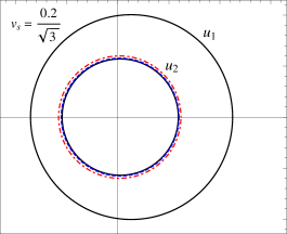
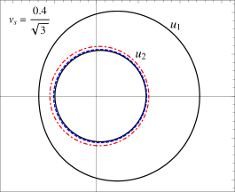
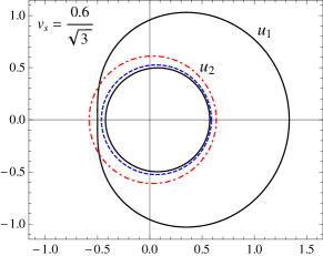
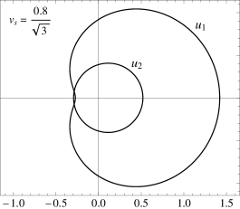
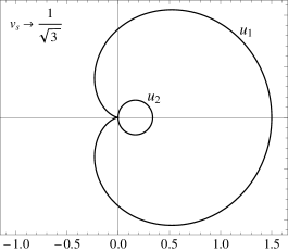
Figure 1: Velocities of first and second sound $u_{1}$, $u_{2}$ from Eqs. (85) for six different values of the superfluid velocity $|{\bf v}_{s}|$ between 0 and $1/\sqrt{3}$. All velocities are measured in the normal-fluid rest frame. In these polar plots, the sound velocities for a given angle between the direction of the wave vector and the superflow are given by the radial distance of the curve to the origin; the direction of the superflow is parallel to the horizontal axis and points to the right; the scale is normalized to the velocity of first sound in the absence of a superflow, as one can see in the upper left panel. The speed of first sound does not depend on temperature within our approximation. The speed of second sound is shown for three different temperatures: $T=0$ [(black) solid], $T/\mu=0.02$ [(blue) dashed], $T/\mu=0.04$ [(red) dashed-dotted]. For large superfluid velocities the temperature expansion breaks down, and we have only shown the results for $T=0$.

We plot the two sound velocities for all angles and for various superfluid velocities in Fig. 1. Because of the breakdown of the temperature expansion we have just explained, the results for nonzero temperature are only shown up to a superfluid velocity where the $T^{2}$ correction is still smaller than the $T=0$ term. We see that both sound velocities are increased when they propagate parallel to the superflow and decreased when they propagate in the opposite direction. At $T=0$, where the result can be taken seriously for all $|{\bf v}_{s}|<1/\sqrt{3}$, the speed of second sound decreases significantly when the critical velocity is approached, and goes to zero for all “backward” angles $\pi/2<\theta<3\pi/2$ (while the velocity of first sound only goes to zero for propagation exactly antiparallel to the superflow, $\theta=\pi$). Interestingly, for a given superfluid velocity, the temperature effect always increases the speed of second sound for all angles. We know that for larger temperatures it must decrease again, because it has to vanish at the critical temperature where there is only one fluid in the system. Within our low-temperature approximation we cannot see this decrease.

VII Summary and outlook

We have discussed the dissipationless hydrodynamics of a relativistic superfluid, starting from a complex scalar field. Our main goal has been to relate the field theory with the covariant two-fluid framework of superfluidity, motivated by quark superfluidity in the CFL phase and its astrophysical relevance. Our results can be summarized as follows.

• Microscopic calculation. We have started from Bose-Einstein condensation in a $\varphi^{4}$ theory. The condensate has been assumed to be static and homogeneous (which corresponds to the simple hydrodynamic scenario of a static, homogeneous superflow). A crucial role is played by the phase of the condensate. While small oscillations of the phase correspond to the excitations of the Goldstone mode, rotations of the phase around the full $U(1)$ circle give rise to a chemical potential (speed of the rotation) and a superfluid three-velocity (number of rotations per unit length). In the presence of a non-zero superflow, the excitations of the Goldstone mode become anisotropic, and we have computed the resulting components of the conserved current and stress-energy tensor for nonzero temperatures. We have restricted ourselves to a weak-coupling, small-temperature approximation, including terms up to sixth order in the temperature. This has allowed us to present the microscopic results in an analytical form. For a study of arbitrary temperatures up to the critical temperature, a more elaborate, self-consistent calculation must be performed numerically.

• Two-fluid formalism. In the relativistic two-fluid formalism, the basic variables are the charge current and the entropy current. In the dissipationless case, both are conserved. For both currents, we can define conjugate momenta. Now, if the two fluids are interacting with each other, neither of the currents is (four-)parallel to its own momentum, but also receives a contribution from the other momentum. This contribution is called entrainment, and it must be computed from an underlying microscopic theory. We have explained this formalism in detail, and in particular have shown the connection to other, equivalent, formulations in the literature. For instance, the entrainment coefficient (and related coefficients) can be expressed in terms of the superfluid and normal-fluid charge densities $n_{n}$ and $n_{s}$ (whose corresponding superfluid and normal-fluid four-currents are, even in the dissipationless case, not separately conserved).

• Relationship between them. There are several concepts and quantities in the two-fluid formalism that are usually not used in field theory, such as the generalized pressure that depends on Lorentz scalars. Therefore, one important aspect of this work has been a translation of these quantities into field-theoretic language. For instance, we have proven that, once we assume that the microscopic calculation is performed in the rest frame of the normal fluid, it follows that the generalized pressure is given by the effective action. We have also expressed the coefficients that relate the currents with the conjugate momenta in terms of quantities that are well defined in field theory, namely the space-time derivative of the phase of the condensate, the components of the Noether current, and the entropy. As a result, we have been able to compute these coefficients explicitly as a function of temperature, chemical potential, and superfluid velocity. Certain combinations of these coefficients yield $n_{n}$ and $n_{s}$. Our calculation shows for instance that $n_{s}$ is not simply given by the condensate density: even though we have neglected the temperature dependence of the condensate, $n_{s}$ depends on temperature. It also confirms that $n_{n}$ is not identical to the phonon number, as one might naively expect; while the phonon number goes like $T^{3}$ for small temperatures (see for instance Ref. Mannarelli and Manuel (2008)), $n_{n}\propto T^{4}/\mu$.

As an application, we have computed the angular and temperature dependent velocities of first and second sound in the presence of a superflow. To obtain non-zero-temperature corrections it has turned out to be crucial to go beyond the linear approximation of the dispersion of the Goldstone mode. Cubic corrections in the dispersion give rise to $T^{6}$ corrections in the pressure and $T^{2}$ corrections in the velocity of second sound, while the velocity of first sound remains temperature-independent. We have found that the velocity of second sound increases with small temperatures although eventually, beyond our small-temperature approximation, it must go to zero when the temperature approaches the critical point.

Our study opens up several directions for future studies. The most direct extension of our work is to go to higher temperatures, for instance in the CJT formalism, as we have briefly laid out at the beginning of Sec. III.1. Such a calculation would capture the temperature dependence of the condensate; it would also go beyond the weak-coupling regime because it necessarily resums higher-order diagrams in order to compute the condensate self-consistently. Although such an extension requires a numerical approach, we expect that the identifications with the hydrodynamic quantities such as normal-fluid and superfluid densities should be straightforward with the help of the present work.

It would also be interesting to relax our assumptions of a uniform superflow and of vanishing dissipation, although this appears less straightforward. Non-uniform situations would require us to build a hydrodynamic limit into our calculation, i.e., we would have to approximate the system as locally uniform. Dissipation clearly goes beyond our equilibrium treatment of the field theory, and it would be very interesting to see if a similar translation to the two-fluid picture also works in that more general case.

In a more phenomenological context, our work can be considered as a first step towards a more complete picture of the hydrodynamics of color-flavor locked quark matter. There are several steps in this direction for the future. It would be interesting to include a (small) term in the Lagrangian that breaks the global $U(1)$ symmetry explicitly and see in which sense superfluidity and the two-fluid picture survive. In a sense, this is similar to including dissipative effects because dissipation leads to a non-conservation of the entropy current, while explicit symmetry breaking leads to non-conservation of the charge current. It is also not unlike anomalous hydrodynamics, where the axial anomaly leads to a non-conserved current and which has been discussed in the recent literature Son and Surowka (2009); Landsteiner et al. (2011); Jensen (2012), also in the context of superfluidity Lin (2012); Bhattacharya et al. (2011); Neiman and Oz (2011). The case of a broken symmetry, while also of theoretical interest, is relevant for the kaon-condensed CFL phase, a viable candidate phase of dense quark matter inside a compact star. In this phase the kaon condensate does break a symmetry that is, due to the weak interactions, not exact. It would also be interesting to include both superfluid components of the CFL-$K^{0}$ phase, the one coming from kaon condensation and the one coming from the spontaneous breaking of the $U(1)$ associated with baryon number symmetry. One could start from a fermionic formalism here, since baryon number is spontaneously broken by the quark Cooper pair condensate.

Appendix A Matsubara sum with anisotropic excitation energies

Here we derive the result (30) for the effective action. The calculation shown here is formulated in a general way, such that it is also applicable to the stress-energy tensor and the current in Sec. III.2. In order to perform the Matsubara sum in Eq. (29), we write the determinant of the inverse propagator in terms of its zeros,

$${\rm det}\,S^{-1}(k)=(k_{0}-\epsilon_{1,{\bf k}}^{+})(k_{0}-\epsilon_{1,{\bf k}}^{-})(k_{0}-\epsilon_{2,{\bf k}}^{+})(k_{0}-\epsilon_{2,{\bf k}}^{-})\,.$$ (86)

In the presence of a superflow $\nabla\psi$, the zeros are very complicated. The reason is the linear term in $k_{0}$ in the off-diagonal elements. With the help of Mathematica we obtain analytical, but very lengthy expressions for $\epsilon_{i,{\bf k}}^{\pm}$. For small momenta, we can write

$$\epsilon_{1,{\bf k}}^{\pm} = \pm\sqrt{\frac{\sigma^{2}-m^{2}}{3\sigma^{2}-m^{2}}}\,\zeta_{\pm}(\hat{\mathbf{k}})|{\bf k}|+{\cal O}(|{\bf k}|^{3})\,,$$ (87a)

$$\epsilon_{2,{\bf k}}^{\pm} = \pm\sqrt{2}\sqrt{3\sigma^{2}-m^{2}+2(\nabla\psi)^{2}}+{\cal O}(|{\bf k}|)\,,$$ (87b)

where

$$\zeta^{\pm}(\hat{\mathbf{k}})\equiv\left[\sqrt{1+2\frac{(\nabla\psi)^{2}-(\nabla\psi\cdot\hat{\mathbf{k}})^{2}}{3\sigma^{2}-m^{2}}}\mp\frac{2\partial_{0}\psi\nabla\psi\cdot\hat{\mathbf{k}}}{\sqrt{\sigma^{2}-m^{2}}\sqrt{3\sigma^{2}-m^{2}}}\right]\left[1+\frac{2(\nabla\psi)^{2}}{3\sigma^{2}-m^{2}}\right]^{-1}\,.$$ (88)

We now use the Matsubara sum

$$T\sum_{k_{0}}\frac{F(k_{0},{\bf k})}{{\rm det}\,S^{-1}(k)} = -\frac{1}{2}\sum_{e=\pm}\sum_{i=1,2}\frac{F(\epsilon_{i,{\bf k}}^{e},{\bf k})}{(\epsilon_{i,{\bf k}}^{e}-\epsilon_{i,{\bf k}}^{-e})(\epsilon_{i,{\bf k}}^{e}-\epsilon_{j,{\bf k}}^{e})(\epsilon_{i,{\bf k}}^{e}-\epsilon_{j,{\bf k}}^{-e})}\coth\frac{\epsilon_{i,{\bf k}}^{e}}{2T}$$ (89)

with $j=2$ if $i=1$ and vice versa, and an arbitrary function $F(k_{0},{\bf k})$ (without poles in the complex $k_{0}$ plane). For the effective action, $F(k_{0},{\bf k})$ is given by Eq. (31), for the stress-energy tensor and the current see Eqs. (44). Since we are interested in small temperatures, we may neglect the contribution from the massive mode, i.e., the two of the four terms in the sum where $i=2$. More precisely: later, after writing $\coth[\epsilon_{i,{\bf k}}^{e}/(2T)]=1+2f(\epsilon_{i,{\bf k}}^{e})$ with the Bose distribution $f$, we shall only keep the thermal contribution, which, in the case of the massive mode, is suppressed for small temperatures. For the non-thermal (divergent) contribution, all terms have to be kept in principle. However, after renormalization, the contribution is subleading since it contains an additional factor of the coupling constant $\lambda$ and we shall neglect it. Therefore, after taking the thermodynamic limit, we can write

$$\frac{T}{V}\sum_{k}\frac{F(k_{0},{\bf k})}{{\rm det}\,S^{-1}(k)} \simeq -\frac{1}{2}\int\frac{d^{3}{\bf k}}{(2\pi)^{3}}\frac{F(\epsilon_{1,{\bf k}}^{+},{\bf k})}{(\epsilon_{1,{\bf k}}^{+}-\epsilon_{1,{\bf k}}^{-})(\epsilon_{1,{\bf k}}^{+}-\epsilon_{2,{\bf k}}^{+})(\epsilon_{1,{\bf k}}^{+}-\epsilon_{2,{\bf k}}^{-})}\coth\frac{\epsilon_{1,{\bf k}}^{+}}{2T}$$ (90)

$$-\,\frac{1}{2}\int\frac{d^{3}{\bf k}}{(2\pi)^{3}}\frac{F(\epsilon_{1,{\bf k}}^{-},{\bf k})}{(\epsilon_{1,{\bf k}}^{-}-\epsilon_{1,{\bf k}}^{+})(\epsilon_{1,{\bf k}}^{-}-\epsilon_{2,{\bf k}}^{+})(\epsilon_{1,{\bf k}}^{-}-\epsilon_{2,{\bf k}}^{-})}\coth\frac{\epsilon_{1,{\bf k}}^{-}}{2T}$$

$$= -\int\frac{d^{3}{\bf k}}{(2\pi)^{3}}\frac{F(\epsilon_{1,{\bf k}}^{+},{\bf k})}{(\epsilon_{1,{\bf k}}^{+}+\epsilon_{1,-{\bf k}}^{+})(\epsilon_{1,{\bf k}}^{+}+\epsilon_{2,-{\bf k}}^{+})(\epsilon_{1,{\bf k}}^{+}-\epsilon_{2,{\bf k}}^{+})}\,\coth\frac{\epsilon_{1,{\bf k}}^{+}}{2T}\,,$$

where, in the last step, we have changed the integration variable of the second integral ${\bf k}\to-{\bf k}$, and have used $F(k_{0},{\bf k})=F(-k_{0},-{\bf k})$ as well as

$$\epsilon_{i,-{\bf k}}^{+}=-\epsilon_{i,{\bf k}}^{-}\,.$$ (91)

This relation is easily checked for the small-momentum expressions (87), and also holds for the full results. Due to the symmetries with respect to reflection of ${\bf k}$, the poles $\epsilon_{i,{\bf k}}^{-}$ have thus dropped out of the result, and the only physical excitations are $\epsilon_{i,{\bf k}}^{+}$. Therefore, in the main text, we have simply denoted $\epsilon_{i,{\bf k}}\equiv\epsilon_{i,{\bf k}}^{+}$ and $\zeta(\hat{\mathbf{k}})\equiv\zeta^{+}(\hat{\mathbf{k}})$.

Appendix B Renormalization and useful identities for stress-energy tensor

With the function $\Psi_{k}$ from Eq. (38) we can write the effective action (27) as

$$\frac{T}{V}\Gamma=-U+\frac{T}{V}\sum_{k}\Psi_{k}\,.$$ (92)

On the other hand, using Eq. (29), we have

$$\frac{T}{V}\Gamma = -U+\frac{1}{3}\frac{T}{V}\sum_{k}\left(C_{k}{\bf k}^{2}-A_{k}{\bf k}\cdot\nabla\psi\right)$$ (93)

$$= -U-\frac{1}{3}(g^{\mu\nu}-u^{\mu}u^{\nu})\frac{T}{V}\sum_{k}\left(C_{k}k_{\mu}k_{\nu}+A_{k}k_{\mu}\partial_{\nu}\psi\right)\,,$$

with the four-vector $u^{\mu}=(1,0,0,0)$ and $A_{k}$, $B_{k}$, $C_{k}$ given in Eq. (39). A useful relation between $A_{k}$, $B_{k}$, $C_{k}$ can be derived with the help of the explicit form of the determinant of the inverse tree-level propagator,

$$1 = \frac{k^{4}-2k^{2}(\sigma^{2}-m^{2})-4(k\cdot\partial\psi)^{2}}{{\rm det}\,S^{-1}}$$ (94)

$$= -\frac{1}{2}[C_{k}k^{2}+B_{k}\sigma^{2}+2A_{k}(k\cdot\partial\psi)]+\frac{k^{2}m^{2}}{{\rm det}\,S^{-1}}\,.$$

Next, we rewrite the stress-energy tensor. With

$$-\frac{T}{V}\sum_{k}{\rm Tr}\left[S\frac{\partial S^{-1}}{\partial g_{\mu\nu}}\right]=2\frac{T}{V}\sum_{k}\frac{\partial\Psi_{k}}{\partial g_{\mu\nu}}$$ (95)

we can write the stress-energy tensor from Eq. (36a) as

$$T^{\mu\nu}=-\left(2\frac{\partial U}{\partial g_{\mu\nu}}-g^{\mu\nu}U\right)+\frac{T}{V}\sum_{k}\left[C_{k}k^{\mu}k^{\nu}+B_{k}\partial^{\mu}\psi\partial^{\nu}\psi+A_{k}(k^{\mu}\partial^{\nu}\psi+k^{\nu}\partial^{\nu}\psi)+g^{\mu\nu}+Y^{\mu\nu}\right]\,,$$ (96)

where we have used the definition of $\Psi_{k}$ (38) and have added a constant, diagonal tensor $Y^{\mu\nu}$ which has to be determined such that the conditions (37) are fulfilled. In order to implement these conditions we now set $\nabla\psi=0$ and $\partial_{0}\psi=\mu$. In this case, because of the first line of Eq. (93), the pressure $P=\frac{T}{V}\Gamma$ becomes

$$P=-U+\frac{1}{3}\frac{T}{V}\sum_{k}C_{k}{\bf k}^{2}\,.$$ (97)

In order to compute the energy density $\epsilon=-P+\mu n+Ts$ we need

$$n = \frac{\partial P}{\partial\mu}=-\frac{\partial U}{\partial\mu}+\frac{T}{V}\sum_{k}(B_{k}\mu+A_{k}k_{0})\,,$$ (98a)

$$s = \frac{\partial P}{\partial T}=-\frac{\partial U}{\partial T}+\frac{P}{T}+\frac{T}{V}\sum_{k}\left(2+A_{k}\frac{\mu k_{0}}{T}+C_{k}\frac{k_{0}^{2}}{T}\right)\,,$$ (98b)

where we have used the form of the pressure (92) and $\partial k_{0}/\partial T=k_{0}/T$ (due to the linear temperature-dependence of the Matsubara frequencies). Consequently,

$$\epsilon=\frac{T}{V}\sum_{k}\left(B_{k}\mu^{2}+2A_{k}k_{0}\mu+C_{k}k_{0}^{2}+2\right)\,.$$ (99)

On the other hand, the nonzero components of the stress-energy tensor without superflow are, from Eq. (96),

$$T^{ij}=\frac{(\mu^{2}-m^{2})^{2}}{4\lambda}\delta^{ij}+\frac{T}{V}\sum_{k}\left(C_{k}\frac{{\bf k}^{2}}{3}\delta^{ij}-\delta^{ij}+Y^{ij}\right)\,,$$ (100)

and

$$T^{00}=\frac{(3\mu^{2}+m^{2})(\mu^{2}-m^{2})}{4\lambda}+\frac{T}{V}\sum_{k}\left(B_{k}\mu^{2}+2A_{k}k_{0}\mu+C_{k}k_{0}^{2}+1+Y^{00}\right)\,,$$ (101)

By comparing Eq. (100) with (97) and (101) with (99) we conclude that $Y^{\mu\nu}={\rm diag}(1,1,1,1)$. Inserting this into Eq. (96), we can write the renormalized stress-energy tensor as

$$T^{\mu\nu}=-\left(2\frac{\partial U}{\partial g_{\mu\nu}}-g^{\mu\nu}U\right)+\frac{T}{V}\sum_{k}\left[C_{k}k^{\mu}k^{\nu}+B_{k}\partial^{\mu}\psi\partial^{\nu}\psi+A_{k}(k^{\mu}\partial^{\nu}\psi+k^{\nu}\partial^{\mu}\psi)+2u^{\mu}u^{\nu}\right]\,,$$ (102)

with $u^{\mu}=(1,0,0,0)$.

Appendix C Small-temperature expansion

Here we explain the small-temperature expansion needed in Sec. III.3 for the effective action, the stress-energy tensor, and the current density. We focus on the effective action in this appendix, but the other results are obtained analogously.

Expanding in powers of the temperature corresponds to expanding the integrand in powers of $|{\bf k}|$. In order to obtain the result up to $T^{6}$, we expand the integrand of the momentum integral in Eq. (30) as

$$\frac{F(\epsilon_{1,{\bf k}},{\bf k})}{(\epsilon_{1,{\bf k}}+\epsilon_{1,-{\bf k}})(\epsilon_{1,{\bf k}}+\epsilon_{2,-{\bf k}})(\epsilon_{1,{\bf k}}-\epsilon_{2,{\bf k}})}\simeq a_{1}|{\bf k}|+\frac{a_{2}}{\sigma^{2}}|{\bf k}|^{3}\,,$$ (103)

and, for the dispersion in the argument of the Bose distribution,

$$\epsilon_{1,{\bf k}}\simeq c_{1}|{\bf k}|+\frac{c_{2}}{\sigma^{2}}|{\bf k}|^{3}\,,$$ (104)

where $a_{1}$, $a_{2}$, $c_{1}$, $c_{2}$ are angular-dependent, dimensionless coefficients. Inserting these expansions, introducing a dimensionless integration variable $y=c_{1}|{\bf k}|/T$, expanding in $T/\sigma$, and performing the resulting integration over $y$ yields

$$\frac{T}{V}\Gamma\simeq\frac{(\sigma^{2}-m^{2})^{2}}{4\lambda}+\frac{2\pi^{2}T^{4}}{45}\int\frac{d\Omega}{4\pi}\left[\frac{a_{1}}{c_{1}^{4}}+\frac{40\pi^{2}}{7c_{1}^{6}}\left(\frac{a_{2}}{3}-\frac{2a_{1}c_{2}}{c_{1}}\right)\frac{T^{2}}{\sigma^{2}}\right]\,,$$ (105)

where we have used the integrals

$$\int_{0}^{\infty}dy\frac{y^{3}}{e^{y}-1}=\frac{\pi^{4}}{15}\,,\qquad\int_{0}^{\infty}dy\frac{y^{5}}{e^{y}-1}=\frac{8\pi^{6}}{63}\,,\qquad\int_{0}^{\infty}dy\frac{y^{6}e^{y}}{(e^{y}-1)^{2}}=\frac{16\pi^{6}}{21}\,.$$ (106)

For the case without superflow, $\nabla\psi=0$, the angular integral becomes trivial. In this case, with $\partial_{0}\psi=\mu$, the full dispersions are given by Eq. (45), and we have

$$c_{1}=\sqrt{\frac{\mu^{2}-m^{2}}{3\mu^{2}-m^{2}}}\,,\qquad c_{2}=\frac{\mu^{6}}{\sqrt{\mu^{2}-m^{2}}(3\mu^{2}-m^{2})^{5/2}}\,,$$ (107)

and

$$a_{1}=\frac{c_{1}}{4}\,,\qquad a_{2}=\frac{3c_{1}}{4}\,.$$ (108)

We thus find for the pressure

$$P=\frac{T}{V}\Gamma \simeq \frac{(\mu^{2}-m^{2})^{2}}{4\lambda}+\frac{\pi^{2}T^{4}}{90c_{1}^{3}}-\frac{4c_{2}\pi^{4}T^{6}}{63\mu^{2}c_{1}^{6}}$$ (109)

$$= \frac{(\mu^{2}-m^{2})^{2}}{4\lambda}+\frac{(3\mu^{2}-m^{2})^{3/2}}{(\mu^{2}-m^{2})^{3/2}}\frac{\pi^{2}T^{4}}{90}-\frac{\mu^{6}(3\mu^{2}-m^{2})^{1/2}}{(\mu^{2}-m^{2})^{7/2}}\frac{4\pi^{4}T^{6}}{63\mu^{2}}\,.$$

The expressions for the case with superflow are quite lengthy in general, and we give the final results in the limit $m=0$ in the main text, see Table 1.

Appendix D Calculation of sound velocities

D.1 Derivation of sound wave equations

We start from the hydrodynamic equations

$$0 = \partial_{\mu}j^{\mu}\,,$$ (110a)

$$0 = \partial_{\mu}s^{\mu}\,,$$ (110b)

$$0 = s_{\mu}(\partial^{\mu}\Theta^{\nu}-\partial^{\nu}\Theta^{\mu})\,.$$ (110c)

Before we evaluate them, we collect some useful relations. We denote $P\equiv P_{n}+P_{s}=\Psi$ and thus can write with Eq. (55)

$$dP = j^{\mu}d(\partial_{\mu}\psi)+s^{\mu}d\Theta_{\mu}$$ (111)

$$= nd\mu+sdT-\frac{n_{s}}{\sigma}\nabla\psi\cdot d\nabla\psi+\frac{n_{n}}{s}{\bf s}\cdot d\nabla\psi-{\bf s}\cdot d\left(\frac{n_{n}}{s}\nabla\psi\right)-{\bf s}\cdot d\left(\frac{w}{s^{2}}{\bf s}\right)\,,$$

where $j^{0}=n$, $s^{0}=s$, $\partial^{0}\psi=\mu$, $\Theta^{0}=T$, and we have eliminated ${\bf j}$ and ${\bf\Theta}$ by using

$$j^{\mu}=n_{n}u^{\mu}+n_{s}\frac{\partial^{\mu}\psi}{\sigma}\,,\qquad\Theta^{\mu}=-\frac{n_{n}}{s}\partial^{\mu}\psi+\frac{w}{s}u^{\mu}\,,$$ (112)

where $w\equiv\epsilon_{n}+P_{n}=\mu n_{n}+sT$ is the enthalpy density of the normal fluid. In the linear approximation, ${\bf s}$ times a space-time derivative is negligible, because ${\bf s}=s^{0}{\bf v}_{n}$ and we neglect products of ${\bf v}_{n}$ with space-time derivatives. Therefore, we may approximate

$$dP \simeq nd\mu+sdT-\frac{n_{s}}{\sigma}\nabla\psi\cdot d\nabla\psi\,.$$ (113)

This relation is needed to express derivatives of any thermodynamic quantity in terms of derivatives of $T$, $\mu$, and $\nabla\psi$. For instance, we can write $\partial_{0}n=\partial_{0}\frac{\partial P}{\partial\mu}=\frac{\partial}{\partial\mu}\partial_{0}P$ etc. and obtain the following useful identities,

$$\partial_{0}n = \frac{\partial n}{\partial\mu}\partial_{0}\mu+\frac{\partial s}{\partial\mu}\partial_{0}T-\frac{\partial(n_{s}/\sigma)}{\partial\mu}\nabla\psi\cdot\nabla\mu\,,$$ (114a)

$$\partial_{0}s = \frac{\partial n}{\partial T}\partial_{0}\mu+\frac{\partial s}{\partial T}\partial_{0}T-\frac{\partial(n_{s}/\sigma)}{\partial T}\nabla\psi\cdot\nabla\mu\,,$$ (114b)

$$\partial_{0}\left(\frac{n_{s}}{\sigma}\partial_{i}\psi\right) = -\frac{\partial n}{\partial(\partial_{i}\psi)}\partial_{0}\mu-\frac{\partial s}{\partial(\partial_{i}\psi)}\partial_{0}T+\frac{\partial(n_{s}/\sigma)}{\partial(\partial_{i}\psi)}\nabla\psi\cdot\nabla\mu+\frac{n_{s}}{\sigma}\partial_{i}\mu\,,$$ (114c)

$$\nabla\cdot\left(\frac{n_{s}}{\sigma}\nabla\psi\right) = -\frac{\partial n}{\partial(\partial_{i}\psi)}\partial_{i}\mu-\frac{\partial s}{\partial(\partial_{i}\psi)}\partial_{i}T+\frac{\partial(n_{s}/\sigma)}{\partial(\partial_{i}\psi)}\partial_{j}\psi\partial_{i}\partial_{j}\psi+\frac{n_{s}}{\sigma}\Delta\psi\,,$$ (114d)

where $\partial_{0}\psi=\mu$ has been used. With these preparations we can discuss the hydrodynamic equations. The current conservation (110a) obviously becomes

$$0\simeq\partial_{0}n+n_{n}\nabla\cdot{\bf v}_{n}-\nabla\cdot\left(\frac{n_{s}}{\sigma}\nabla\psi\right)\,,$$ (115)

where we have used ${\bf u}\simeq{\bf v}_{n}$ and $\nabla\cdot(n_{n}{\bf v}_{n})\simeq n_{n}\nabla\cdot{\bf v}_{n}$. Inserting Eqs. (114a) and (114d) into this equation, taking the time derivative of the result, and multiplying the whole equation by $\mu$ yields

$$0 \simeq \mu\frac{\partial n}{\partial\mu}\partial_{0}^{2}\mu+\mu\frac{\partial s}{\partial\mu}\partial_{0}^{2}T-n_{s}\frac{\mu}{\sigma}\Delta\mu+\mu n_{n}\nabla\cdot\partial_{0}{\bf v}_{n}-\mu\frac{\partial(n_{s}/\sigma)}{\partial\mu}\nabla\psi\cdot\nabla\partial_{0}\mu$$ (116)

$$+\mu\frac{\partial n}{\partial(\partial_{i}\psi)}\partial_{0}\partial_{i}\mu+\mu\frac{\partial s}{\partial(\partial_{i}\psi)}\partial_{0}\partial_{i}T-\mu\frac{\partial(n_{s}/\sigma)}{\partial(\partial_{i}\psi)}\partial_{j}\psi\partial_{i}\partial_{j}\mu\,.$$

Due to the linear approximation, all expressions have the form (equilibrium quantity) $\times$ (second space-time derivative), since products of two first space-time derivatives are of higher order.

The entropy conservation (110b) reads

$$0\simeq\partial_{0}s+s\nabla\cdot{\bf v}_{n}\,.$$ (117)

Inserting Eq. (114b), taking the time derivative of the result and multiplying the whole equation by $T$ yields

$$0\simeq T\frac{\partial n}{\partial T}\partial_{0}^{2}\mu+T\frac{\partial s}{\partial T}\partial_{0}^{2}T-T\frac{\partial(n_{s}/\sigma)}{\partial T}\nabla\psi\cdot\nabla\partial_{0}\mu+sT\nabla\cdot\partial_{0}{\bf v}_{n}\,.$$ (118)

It is convenient for the following to add Eqs. (116) and (118),

$$0 \simeq \left(\mu\frac{\partial n}{\partial\mu}+T\frac{\partial n}{\partial T}\right)\partial_{0}^{2}\mu+\left(\mu\frac{\partial s}{\partial\mu}+T\frac{\partial s}{\partial T}\right)\partial_{0}^{2}T-\left[\mu\frac{\partial(n_{s}/\sigma)}{\partial\mu}+T\frac{\partial(n_{s}/\sigma)}{\partial T}\right]\nabla\psi\cdot\nabla\partial_{0}\mu+w\nabla\cdot\partial_{0}{\bf v}_{n}$$ (119)

$$+2\mu\frac{\partial n}{\partial(\nabla\psi)^{2}}\nabla\psi\cdot\nabla\partial_{0}\mu+2\mu\frac{\partial s}{\partial(\nabla\psi)^{2}}\nabla\psi\cdot\nabla\partial_{0}T-2\mu\frac{\partial(n_{s}/\sigma)}{\partial(\nabla\psi)^{2}}(\nabla\psi\cdot\nabla)^{2}\mu-n_{s}\frac{\mu}{\sigma}\Delta\mu\,,$$

where we have rewritten the derivative with respect to $\partial_{i}\psi$ in terms of the derivative with respect to $(\nabla\psi)^{2}$.

Finally, we need the vorticity equation (110c). The temporal component becomes

$$0={\bf s}\cdot(\nabla T+\partial_{0}{\bf\Theta})\,.$$ (120)

We can neglect this equation completely, since in both terms the normal fluid velocity is multiplied with a space-time derivative. The spatial components are

$$0\simeq s(\partial_{0}{\bf\Theta}+\nabla T)\simeq s\nabla T+w\partial_{0}{\bf v}_{n}+s\partial_{0}\left(\frac{n_{n}}{s}\nabla\psi\right)\,,$$ (121)

where ${\bf\Theta}$ from Eq. (112) has been used. The last term needs some rearrangements,

$$s\partial_{0}\left(\frac{n_{n}}{s}\nabla\psi\right) = -\frac{n_{n}}{s}\nabla\psi\,\partial_{0}s+\partial_{0}(n_{n}\nabla\psi)=-\frac{n_{n}}{s}\nabla\psi\,\partial_{0}s+\partial_{0}(n\nabla\psi)-\partial_{0}\left(n_{s}\frac{\mu}{\sigma}\nabla\psi\right)$$ (122)

$$= -\frac{n_{n}}{s}\nabla\psi\,\partial_{0}s+\nabla\psi\partial_{0}n+n\nabla\mu-\frac{n_{s}}{\sigma}\nabla\psi\partial_{0}\mu-\mu\partial_{0}\left(\frac{n_{s}}{\sigma}\nabla\psi\right)\,.$$

Inserting Eqs. (114a), (114b), and (114c) into this relation, the result into Eq. (121), and taking the divergence of the resulting equation, we arrive at

$$0 \simeq n_{n}\Delta\mu+s\Delta T+w\nabla\cdot\partial_{0}{\bf v}_{n}-\frac{n_{s}}{\sigma}\nabla\psi\cdot\nabla\partial_{0}\mu-\left[\frac{n_{n}}{s}\frac{\partial n}{\partial T}-\frac{\partial n}{\partial\mu}-2\mu\frac{\partial n}{\partial(\nabla\psi)^{2}}\right]\nabla\psi\cdot\nabla\partial_{0}\mu$$ (123)

$$-\left[\frac{n_{n}}{s}\frac{\partial s}{\partial T}-\frac{\partial s}{\partial\mu}-2\mu\frac{\partial s}{\partial(\nabla\psi)^{2}}\right]\nabla\psi\cdot\nabla\partial_{0}T+\left[\frac{n_{n}}{s}\frac{\partial(n_{s}/\sigma)}{\partial T}-\frac{\partial(n_{s}/\sigma)}{\partial\mu}-2\mu\frac{\partial(n_{s}/\sigma)}{\partial(\nabla\psi)^{2}}\right](\nabla\psi\cdot\nabla)^{2}\mu\,.$$

The normal fluid velocity can now be eliminated by solving this relation for $\nabla\cdot\partial_{0}{\bf v}_{n}$ and inserting the result into the other two equations: inserting it into Eq. (118) yields, after multiplying the whole equation with $w/(Ts)$, Eq. (82a) in the main text, while inserting it into Eq. (119) yields Eq. (82b). These are the sound wave equations from which the sound velocities are computed as follows.

D.2 Solution of sound wave equations

Replacing the chemical potential and the temperature in all space-time derivatives of the sound wave equations (82) by $\delta\mu=\delta\mu_{0}e^{i(\omega t-{\bf k}\cdot{\bf x})}$ and $\delta T=\delta T_{0}e^{i(\omega t-{\bf k}\cdot{\bf x})}$, the sound wave equations become

$$0 \simeq \left[a_{1}\tilde{\omega}^{2}+(a_{2}+a_{4}\mu^{2}{\bf v}_{s}^{2}\cos^{2}\theta)+a_{3}\mu|{\bf v}_{s}|\tilde{\omega}\cos\theta\right]\delta\mu_{0}+(b_{1}\tilde{\omega}^{2}+b_{2}+b_{3}\mu|{\bf v}_{s}|\tilde{\omega}\cos\theta)\,\delta T_{0}\,,$$ (124a)

$$0 \simeq \left[A_{1}\tilde{\omega}^{2}+(A_{2}+A_{4}\mu^{2}{\bf v}_{s}^{2}\cos^{2}\theta)+A_{3}\mu|{\bf v}_{s}|\tilde{\omega}\cos\theta\right]\delta\mu_{0}+(B_{1}\tilde{\omega}^{2}+B_{2}+B_{3}\mu|{\bf v}_{s}|\tilde{\omega}\cos\theta)\,\delta T_{0}\,,$$ (124b)

where $\cos\theta\equiv\hat{\mathbf{k}}\cdot\hat{\bf v}_{s}$, $\tilde{\omega}\equiv\omega/|{\bf k}|$, and we have abbreviated

$$a_{1} \equiv \frac{w}{s}\frac{\partial n}{\partial T}\,,\qquad a_{2}\equiv-n_{n}\,,\qquad a_{3}\equiv\frac{n_{s}}{\sigma}-\frac{w}{s}\frac{\partial(n_{s}/\sigma)}{\partial T}+\frac{n_{n}}{s}\frac{\partial n}{\partial T}-\frac{\partial n}{\partial\mu}-2\mu\frac{\partial n}{\partial(\nabla\psi)^{2}}\,,$$

$$a_{4} \equiv -\left[\frac{n_{n}}{s}\frac{\partial(n_{s}/\sigma)}{\partial T}-\frac{\partial(n_{s}/\sigma)}{\partial\mu}-2\mu\frac{\partial(n_{s}/\sigma)}{\partial(\nabla\psi)^{2}}\right]\,,$$ (125a)

$$b_{1} \equiv \frac{w}{s}\frac{\partial s}{\partial T}\,,\qquad b_{2}\equiv-s\,,\qquad b_{3}\equiv\frac{n_{n}}{s}\frac{\partial s}{\partial T}-\frac{\partial s}{\partial\mu}-2\mu\frac{\partial s}{\partial(\nabla\psi)^{2}}\,,$$ (125b)

$$A_{1} \equiv \mu\frac{\partial n}{\partial\mu}+T\frac{\partial n}{\partial T}\,,\qquad A_{2}\equiv-n\,,\qquad A_{3}\equiv\frac{n_{s}}{\sigma}-\mu\frac{\partial(n_{s}/\sigma)}{\partial\mu}-T\frac{\partial(n_{s}/\sigma)}{\partial T}+\frac{n_{n}}{s}\frac{\partial n}{\partial T}-\frac{\partial n}{\partial\mu}\,,$$

$$A_{4} \equiv -\left[\frac{n_{n}}{s}\frac{\partial(n_{s}/\sigma)}{\partial T}-\frac{\partial(n_{s}/\sigma)}{\partial\mu}\right]$$ (125c)

$$B_{1} \equiv \mu\frac{\partial s}{\partial\mu}+T\frac{\partial s}{\partial T}\,,\qquad B_{2}\equiv-s\,,\qquad B_{3}\equiv\frac{n_{n}}{s}\frac{\partial s}{\partial T}-\frac{\partial s}{\partial\mu}\,.$$ (125d)

In general, the determinant of the coefficient matrix of the system of two equations (124) yields a complicated quartic equation for $\tilde{\omega}$. However, we can simplify the result as follows. First one can check, for instance by explicit calculation, that the temperature dependence of the various coefficients is

$$a_{i}=a_{i}^{(4)}T^{4}+a_{i}^{(6)}T^{6}\,,\quad A_{i}=A_{i}^{(0)}+A_{i}^{(4)}T^{4}+A_{i}^{(6)}T^{6}\,,\quad b_{j}=b_{j}^{(3)}T^{3}+b_{j}^{(5)}T^{5}\,,\quad B_{j}=B_{j}^{(3)}T^{3}+B_{j}^{(5)}T^{5}\,,$$ (126)

where $i=1,2,3,4$, $j=1,2,3$, and where the prefactors in front of the various powers of $T$ depend on the superfluid velocity ${\bf v}_{s}$. Since we have computed the pressure up to order $T^{6}$, all terms of order $T^{7}$ and higher must be neglected in these expressions. We see in particular that only the $A_{i}$’s contribute in the limit $T=0$. Now, for the determinant we encounter two kinds of products, namely $A_{i}b_{j}$ and $a_{i}B_{j}$,

$$A_{i}b_{j} = T^{3}[A_{i}^{(0)}+A_{i}^{(4)}T^{4}+A_{i}^{(6)}T^{6}][b_{j}^{(3)}+b_{j}^{(5)}T^{2}]=T^{3}A_{i}^{(0)}[b_{j}^{(3)}+b_{j}^{(5)}T^{2}]+{\cal O}(T^{7})\,,$$ (127a)

$$a_{i}B_{j} = T^{7}[a_{i}^{(4)}+a_{i}^{(6)}T^{2}][B_{j}^{(3)}+B_{j}^{(5)}T^{2}]={\cal O}(T^{7})\,.$$ (127b)

The first line shows that the ${\cal O}(T^{7})$ terms are unknown in our expansion because a $b_{j}^{(7)}T^{7}$ term in $b_{j}$ would give rise to a $T^{7}$ term in $A_{i}b_{j}$, but we have not computed $b_{j}^{(7)}$. Therefore, we must neglect all products of the form given in the second line since they are all of order $T^{7}$ and higher. In other words, it is consistent with our approximation to set $a_{i}\simeq B_{i}\simeq 0$ and use the $T=0$ results for $A_{i}$. In this case the quartic equation for $\omega$ factorizes into two quadratic equations,

$$0 \simeq A_{1}^{(0)}\tilde{\omega}^{2}+(A_{2}^{(0)}+A_{4}^{(0)}\mu^{2}{\bf v}_{s}^{2}\cos^{2}\theta)+A_{3}^{(0)}\mu|{\bf v}_{s}|\tilde{\omega}\cos\theta\,,$$ (128a)

$$0 \simeq [b_{1}^{(3)}+b_{1}^{(5)}T^{2}]\tilde{\omega}^{2}+[b_{2}^{(3)}+b_{2}^{(5)}T^{2}]+[b_{3}^{(3)}+b_{3}^{(5)}T^{2}]\mu|{\bf v}_{s}|\tilde{\omega}\cos\theta\,.$$ (128b)

After dividing out the overall factor $T^{3}$ of the quartic equation, the highest remaining power of temperature is 2, i.e., our approximation allows us to reliably compute the sound velocities up to $T^{2}$. From the first equation we see that one of the solutions has no $T^{2}$ correction. This is the velocity of first sound. The second equation yields the velocity of second sound which does have a $T^{2}$ correction. We see that the coefficients $b_{i}^{(5)}$ are needed to compute this correction. These coefficients arise from the $T^{5}$ terms in the entropy, i.e., from the $T^{6}$ terms in the pressure. Had we truncated our expansion of the pressure at order $T^{4}$, the velocity of second sound would have turned out to be independent of temperature. There are two physical solutions of Eqs. (128), $\omega=u_{1,2}|{\bf k}|$. For the explicit calculation of the two sound velocities $u_{1}$, $u_{2}$ we need $n_{s}$ and $n_{n}$ from Eqs. (79) and the entropy $s$ (obtained by taking the derivative with respect to temperature of $\Psi=T_{\perp}$ from Table 1). The result is given in Eqs. (85) in the main part of the paper.

References

- Tisza (1938) L. Tisza, Nature 141, 913 (1938).
- Kapitza (1938) P. Kapitza, Nature 141, 74 (1938).
- Allen and Misener (1938) J. F. Allen and A. D. Misener, Nature 141, 75 (1938).
- Landau (1941) L. Landau, Phys. Rev. 60, 356 (1941).
- Khalatnikov and Lebedev (1982) I. M. Khalatnikov and V. V. Lebedev, Physics Letters A 91, 70 (1982).
- Lebedev and Khalatnikov (1982) V. V. Lebedev and I. M. Khalatnikov, Zh. Eksp. Teor. Fiz. 83, 1601 (1982), [Sov. Phys. JETP, 56, 923 (1982)].
- Carter (1989) B. Carter, in Relativistic Fluid Dynamics (Noto 1987), edited by A. Anile and M. Choquet-Bruhat (Springer-Verlag, 1989), pp. 1–64.
- Carter and Khalatnikov (1992) B. Carter and I. M. Khalatnikov, Phys. Rev. D 45, 4536 (1992).
- Andersson and Comer (2005) N. Andersson and G. Comer, Living Rev.Rel. 10, 1 (2005), eprint gr-qc/0605010.
- London (1938) F. London, Nature 141, 643 (1938).
- Carter and Langlois (1995) B. Carter and D. Langlois, Phys.Rev. D51, 5855 (1995), eprint hep-th/9507058.
- Comer and Joynt (2003) G. Comer and R. Joynt, Phys.Rev. D68, 023002 (2003), eprint gr-qc/0212083.
- Nicolis (2011) A. Nicolis (2011), eprint 1108.2513.
- Son (2002) D. T. Son (2002), eprint hep-ph/0204199.
- Manuel et al. (2005) C. Manuel, A. Dobado, and F. J. Llanes-Estrada, JHEP 09, 076 (2005), eprint hep-ph/0406058.
- Alford et al. (2007) M. G. Alford, M. Braby, S. Reddy, and T. Schäfer, Phys. Rev. C75, 055209 (2007), eprint nucl-th/0701067.
- Manuel and Llanes-Estrada (2007) C. Manuel and F. Llanes-Estrada, JCAP 0708, 001 (2007), eprint arXiv:0705.3909 [hep-ph].
- Mannarelli and Manuel (2008) M. Mannarelli and C. Manuel, Phys. Rev. D77, 103014 (2008), eprint 0802.0321.
- Alford et al. (2008a) M. G. Alford, M. Braby, and A. Schmitt, J. Phys. G35, 115007 (2008a), eprint 0806.0285.
- Mannarelli and Manuel (2010) M. Mannarelli and C. Manuel, Phys.Rev. D81, 043002 (2010), eprint 0909.4486.
- Alford et al. (1999) M. G. Alford, K. Rajagopal, and F. Wilczek, Nucl. Phys. B537, 443 (1999), eprint hep-ph/9804403.
- Andersson (1998) N. Andersson, Astrophys. J. 502, 708 (1998), eprint gr-qc/9706075.
- Jaikumar et al. (2008) P. Jaikumar, G. Rupak, and A. W. Steiner, Phys.Rev. D78, 123007 (2008), eprint 0806.1005.
- Andersson et al. (2010) N. Andersson, B. Haskell, and G. Comer, Phys.Rev. D82, 023007 (2010), eprint 1005.1163.
- Alford et al. (2012a) M. Alford, S. Mahmoodifar, and K. Schwenzer, Phys.Rev. D85, 024007 (2012a), eprint 1012.4883.
- Alford et al. (2012b) M. G. Alford, S. Mahmoodifar, and K. Schwenzer, Phys.Rev. D85, 044051 (2012b), eprint 1103.3521.
- Epstein (1988) R. I. Epstein, Astrophys. J. 333, 880 (1988).
- Lee (1995) U. Lee, Astron. Astrophys. 303, 515 (1995).
- Langlois et al. (1998) D. Langlois, D. M. Sedrakian, and B. Carter, Mon.Not.Roy.Astron.Soc. 297, 1189 (1998), eprint arXiv:astro-ph/9711042.
- Haskell et al. (2012) B. Haskell, N. Andersson, and G. L. Comer, Phys. Rev. D 86, 063002 (2012), eprint 1204.2894.
- Glampedakis et al. (2012) K. Glampedakis, N. Andersson, and S. K. Lander, Mon.Not.Roy.Astron.Soc. 420, 1263 (2012), eprint 1106.6330.
- Alford et al. (2008b) M. G. Alford, A. Schmitt, K. Rajagopal, and T. Schafer, Rev.Mod.Phys. 80, 1455 (2008b), eprint 0709.4635.
- Bedaque and Schäfer (2002) P. F. Bedaque and T. Schäfer, Nucl. Phys. A697, 802 (2002), eprint hep-ph/0105150.
- Son (2001a) D. T. Son (2001a), eprint hep-ph/0108260.
- Alford et al. (2008c) M. G. Alford, M. Braby, and A. Schmitt, J. Phys. G35, 025002 (2008c), eprint arXiv:0707.2389 [nucl-th].
- Luttinger and Ward (1960) J. M. Luttinger and J. C. Ward, Phys. Rev. 118, 1417 (1960).
- Baym (1962) G. Baym, Phys. Rev. 127, 1391 (1962).
- Cornwall et al. (1974) J. M. Cornwall, R. Jackiw, and E. Tomboulis, Phys. Rev. D10, 2428 (1974).
- Alford et al. (in preparation) M. G. Alford, S. K. Mallavarapu, A. Schmitt, and S. Stetina (in preparation).
- Son (2001b) D. Son, Int.J.Mod.Phys. A16S1C, 1284 (2001b), eprint hep-ph/0011246.
- Gusakov and Andersson (2006) M. E. Gusakov and N. Andersson, Mon.Not.Roy.Astron.Soc. 372, 1776 (2006), eprint astro-ph/0602282.
- Gusakov (2007) M. E. Gusakov, Phys. Rev. D76, 083001 (2007), eprint 0704.1071.
- Herzog et al. (2009) C. Herzog, P. Kovtun, and D. Son, Phys.Rev. D79, 066002 (2009), eprint 0809.4870.
- Herzog and Yarom (2009) C. P. Herzog and A. Yarom, Phys.Rev. D80, 106002 (2009), eprint 0906.4810.
- Andersson and Comer (2011) N. Andersson and G. Comer, Int.J.Mod.Phys. D20, 1215 (2011).
- Israel (1981) W. Israel, Physica A Statistical Mechanics and its Applications 106, 204 (1981).
- Weldon (1982) H. A. Weldon, Phys.Rev. D26, 1394 (1982).
- Taylor et al. (2009) E. Taylor, H. Hu, X.-J. Liu, L. P. Pitaevskii, A. Griffin, and S. Stringari, Phys. Rev. A 80, 053601 (2009), eprint 0905.0257.
- Arahata and Nikuni (2009) E. Arahata and T. Nikuni, Phys. Rev. A 80, 043613 (2009), eprint 0907.2743.
- Hu et al. (2010) H. Hu, E. Taylor, X.-J. Liu, S. Stringari, and A. Griffin, New Journal of Physics 12, 043040 (2010), eprint 1001.0772.
- Bertaina et al. (2010) G. Bertaina, L. Pitaevskii, and S. Stringari, Physical Review Letters 105, 150402 (2010), eprint 1002.0195.
- Meppelink et al. (2009) R. Meppelink, S. B. Koller, and P. van der Straten, Phys. Rev. A 80, 043605 (2009), eprint 0909.3455.
- Arahata et al. (2011) E. Arahata, T. Nikuni, and A. Griffin, Phys. Rev. A 84, 053612 (2011), eprint 1108.2382.
- Adamenko et al. (2009) I. N. Adamenko, K. E. Nemchenko, V. A. Slipko, and A. F. G. Wyatt, Phys. Rev. B 79, 104508 (2009).
- Son and Surowka (2009) D. T. Son and P. Surowka, Phys.Rev.Lett. 103, 191601 (2009), eprint 0906.5044.
- Landsteiner et al. (2011) K. Landsteiner, E. Megias, and F. Pena-Benitez, Phys.Rev.Lett. 107, 021601 (2011), eprint 1103.5006.
- Jensen (2012) K. Jensen, Phys.Rev. D85, 125017 (2012), eprint 1203.3599.
- Lin (2012) S. Lin, Nucl.Phys. A873, 28 (2012), eprint 1104.5245.
- Bhattacharya et al. (2011) J. Bhattacharya, S. Bhattacharyya, S. Minwalla, and A. Yarom (2011), eprint 1105.3733.
- Neiman and Oz (2011) Y. Neiman and Y. Oz, JHEP 1109, 011 (2011), eprint 1106.3576.