Modeling Epidemic Risk Perception in Networks with Community Structure

Abstract

We study the influence of global, local and community-level risk perception on the extinction probability of a disease in several models of social networks. In particular, we study the infection progression as a susceptible-infected-susceptible (SIS) model on several modular networks, formed by a certain number of random and scale-free communities. We find that in the scale-free networks the progression is faster than in random ones with the same average connectivity degree. For what concerns the role of perception, we find that the knowledge of the infection level in one’s own neighborhood is the most effective property in stopping the spreading of a disease, but at the same time the more expensive one in terms of the quantity of required information, thus the cost/effectiveness optimum is a tradeoff between several parameters.

1 Introduction

Epidemic spreading is one of the most successful and most studied applications in the field of complex networks. The comprehension of the spreading behavior of many diseases, like sexually transmitted diseases (i.e. HIV) or the H1N1 virus, can be studied through computational models in complex networks barrat2008 ; Newman2010 . In addition to “real” viruses, spreading of information or computer malware in technological networks is of interest as well.

The susceptible-infected-susceptible (SIS) model is often used to study the spreading of an infectious agent on a network. In this model an individual is represented as a node, which can be either be “healthy” or “infected”. Connections between individuals along which the infection can spread are represented by links. In each time step a healthy node is infected with a certain probability if it is connected to at least one infected node, otherwise it reverts to a healthy node (parallel evolution).

The study of epidemic spreading is a well-known topic in the field of physics and computer science. The dynamics of infectious diseases has been extensively studied in scale-free networks PhysRevE.63.066117 ; PhysRevLett.90.028701 ; PhysRevE.76.061904 ; PhysRevE.66.036113 , in small-world networks PhysRevE.61.5678 and in several kind of regular and random graphs.

A general finding is that it is hard to stop an epidemic in scale-free networks with slow tails, at least in the absence of correlations in the network among the infections process and the node characteristics PhysRevE.63.066117 . This effect is essential due to the presence of hubs, which act like strong spreaders. However, by using an appropriate policy for hubs, it is possible to stop epidemics also in scale-free networks stopping ; PhysRevE.76.061904 .

This network-aware policy is inspired by the behavior of real human societies, in which selection had lead to the development of strategies used to avoid or reduce infections. However, human societies are not structureless, and a particular focus must be devoted to the community structures, which are highly important for our social behavior.

Recently, a wave of studies focused the attention on the effect of the community structure in the modelling of epidemic spreading 10.1371/journal.pcbi.1000736 ; Chen20121848 ; in . However, the focus was only set towards the interaction between the viruses’ features and the topology, without considering the important relation between cognitive strategies used by subjects and the structure of their (local) community/neighborhood.

Considering this scenario, an important challenge is the comprehension of the structure of real-world networks communities ; Girvan02 ; fortunato2007 . Given a graph, a community is a group of vertices that is “more linked” within the group than with the rest of the graph. This is clearly a poor definition, and indeed, in a connected graph, there is not a clear distinction between a community and a rest of the graph. In general, there is a continuum of nested communities whose boundaries are somewhat arbitrary: the structure of communities can be seen as a hierarchical dendrogram Newman .

It is generally accepted that the presence of a community structure plays a crucial role in the dynamics of complex networks; for this reason, lots of energy has been invested to develop algorithms for the detection of communities in networks Fortunato201075 ; Modus ; MCL . However, in complex networks, and in particular in social networks, it is very difficult to give a clear definition of a community: nodes often belong to more than just one cluster or module. The problem of overlapping communities was exposed in Palla and recently analyzed in Lanc . People usually belong to different communities at the same time, depending on their families, friends, colleagues, etc. For instance, if we want to analyze the spreading of sexual diseases in a social environment, it is important to understand the mechanism that leads people to interact with each other. We can surely detect two distinct groups of people (i.e., communities): heterosexual and homosexual, with bisexual people that act as overlapping vertexes between the two principal communities citeulike:3856997 ; gcalda:AM92 ; Chen20121848 .

The strategies used to face the infection spreading in a community is itself a complex process (i.e., social problem solving) in which strategies spread (as the epidemics) along the community, and are negotiated and assumed or discarded depending on their social success.

Several factors can affect the social problem solving which is represented by the adoption of a behaviour to reduce the infection risk. Of course, personality factors, previous experiences and the social and economical states of a subject can be considered as influencing variables. Another important variable is represented by the structure of the environment in which the social communities live, because it determines at the same time the speed of the epidemic diffusion and the strategy of the negotiation process; in particular large and more connected communities are often characterized by conservative strategies while small and isolated communities allow more relaxed strategies.

The same strategy can be more or less effective depending on the strategies adopted by the neighbours (community) of the subject. For instance, a subject in a conservative community can adopt a more risky (and presumably profitable) attitude with a certain confidence since he would be protected from the infection, because of their neighbours’ behaviours, and this “parasitic” behavior (like refusing vaccinations) can be tolerated (up to a certain level) without lowering the community’s fitness.

Not only the neighbor’s behaviour affect the evolution of the cognitive strategies of a subject, but also the position he has in the network should be a relevant factor. A hub, or a subject with a great social betweenness, is usually more exposed to the infection than a leaf, and as a consequence, the best strategy for him has to be different. In the same way, since the topology of the network (e.g., small world, random) determines variables such as the speed of the spreading, or its pervasiveness, it should also affect the development of the “best strategy”.

Moreover, while the negotiation process evolves, the cognitive strategies usually develop within the most intimate community of a subject, thus the behaviour adopted by subjects could be an interesting feature for the community detection problem as well.

The understanding of the effects of the community structure on the epidemic spreading in networks is still an open task. In this paper we investigate the role of risk perception in artificial networks generated in order to reproduce several types of overlapping community structures.

The rest of this paper is organized as follows: we start by describing a mechanism for generating networks with overlapping community structures in section 2. In section 3, we describe the SIS model adopted to model the risk perception of subjects in those networks. Finally, section 4 contains simulation results from our model with a troughout discussion and future work proposals.

2 The networks model

Figure 1: (a) An example network with $4$ different communities composed by $10$ vertices: in this case, considering $p_{1}=1$ and $p_{2}=0$, we generate $4$ non interconnected full connected networks. (b) The same $4$ communities with parameters $p_{1}=0.95$ and $p_{2}=0.05$.

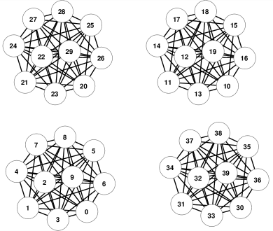
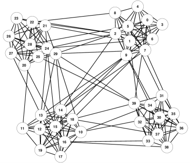
There are $n_{c}$ different communities with $n_{v}$ vertices (in this paper we consider only undirected and unweighted graphs); we assume that the probability to have a link between the vertexes in the same community is $p_{1}$, while $p_{2}$ is the probability to have a link between two nodes belonging to different communities. For instance, with $p_{1}=1$ and $p_{2}=0$, we generate $n_{c}$ fully connected graphs, with no connections among them as shown in figure 1(a). It is possible to use the parameters $p_{1}$ and $p_{2}$ to control the interaction among different communities, as shown in Figure 1(b). The algorithm for generating this kind of networks can be summarized as:

1. Define $s_{1}$ as number of vertexes in the communities;

2. Define $n_{c}$ as number of communities;

3. For all the $n_{c}$ communities create a link between the vertexes on them with probability $p_{1}$;

4. For all the vertexes $N=s_{1}n_{c}$ create a link between them and a random vertex of other communities with probability $p_{2}$;

Figure 2: (a) Random networks: in this figure, we show the frequency distribution of the connectivity degree changing the value of the parameter $p_{2}$. The circles represent the values for $p_{2}=0.01$, crosses for $p_{2}=0.1$ and eventually squares for $p_{2}=0.2$. Here, $s_{1}=1000$ and $n_{c}=5$, thus we have generated networks with $5$ communities of $1000$ nodes for each. (b) Distribution of connectivity degree for the scale-free network generated with the mechanism described above (dots). The straight line is a power law curve with exponent $\gamma=2.5$.

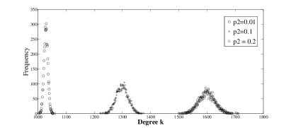
Constraining the condition $p_{1}=1-p_{2}$, we can reduce the free parameters to just one. The connectivity degree itself depends on the size of the network and on the probabilities $p_{1}$ and $p_{2}$. In particular the connectivity function $f(k)$ has a normal distribution from which we could define the mean connectivity $\left\langle k\right\rangle$, as:

$$\left\langle k\right\rangle=(s_{1}-1)p_{1}+(n_{c}-1)s_{1}p_{2}$$ (1)

with standard deviation $\sigma^{2}(k)=(s_{1}-1)p_{1}(1-p_{1})+(n_{c}-1)s_{1}p_{2}(1-p_{2})$.

In figure 2(a) we show the frequency distribution of the connectivity degree of nodes varying the value of the parameter $p_{2}$ for a network composed by $N=5000$ nodes and $n_{c}=5$ communities.

It is widely accepted that real-world networks, from social networks to computer networks are scale-free networks, whose degree distribution follows a power law, at least asymptotically. In this network, the probability distribution of contacts often exhibits a power-law behavior:

$$P(k)\propto ck^{-\gamma},$$ (2)

with an exponent $\gamma$ between $2$ and $3$ sf ; PhysRevLett.85.4633 . For generating networks with this kind of networks we adopt the following mechanism:

1. Start with a fully connected network of $m$ nodes;

2. Add $N-m$ nodes;

3. For each new nodes add $m$ links;

4. For each of these links choose a node at random from the ones already belonging to the network and attach the link to one of the neighbors of that node, if not already attached.

Through this mechanism we are able to generated scale-free networks with an exponent $\gamma{}=2.5$ as shown in figure 2(b). There, we show the frequency distribution of the connectivity degree for a network of $10^{6}$ nodes. To generate a community structure with a realistic distribution, we first generate $n_{c}$ scale-free networks as explained above. Then, for all nodes and all outgoing links, we replace the link pointing inside the community with that connecting a neighbor of a random node in a random community with a probability of $p_{2}=1-p_{1}$. Thus, the algorithm can be summarized as:

1. Generate $n_{c}$ communities as scale-free networks with $n_{v}$ vertices;

2. For all the vertices, with a probability $p_{2}=1-p_{1}$;

   • Delete a random link;

   • Select a random node of another community and create a link with one of its adjacent vertex;

3. End.

Figure 3: Different values of modularity ($Q$) after increasing the mixing parameter $p_{2}$ for two networks with $N=4\cdot 10^{5}$ nodes and $N=4\cdot 10^{2}$ nodes.

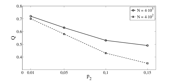
In this way, we are able to generate scale-free networks with a well defined community structure. A good measure for the estimation of the strength of the community structure is the so-called modularity Girvan02 . The modularity $Q$ is defined to be:

$$Q=\frac{1}{2}\sum_{vw}\left[A_{vw}-\frac{K_{v}K_{w}}{2m}\right]\delta(c_{v},c_{w}),$$ (3)

where $A$ is the adjacency matrix in which $A_{vw}=1$ if $w$ and $v$ are connected and $0$ otherwise. $m=\frac{1}{2}\sum_{vw}A_{vw}$ is the number of edges in the graph, $K_{i}$ is the connectivity degree of node $i$ and $(K_{v}K_{w})/(2m)$ represents the probability of an edge existing between vertices $v$ and $w$ if connections are made at random but with respecting vertex degrees. $\delta(c_{v},c_{w})$ is defined as follows:

$$\delta(c_{v},c_{w})=\sum_{r}^{n_{c}}\hat{c}_{vr}\hat{c}_{wr}$$ (4)

where $\hat{c}_{ir}$ is $1$ if vertex $i$ belongs to group $r$, and $0$ otherwise.

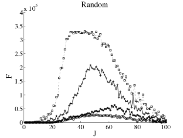
In figure 3 we show the values of modularity for two networks that were generated with the same algorithm, but with different sizes. Here, we consider a network with $4$ communities: in the first case $s_{1}=10^{5}$, while in the second case $s_{1}=10^{2}$. What one can observe in figure 3 is that the modularity’s behaviour does not change significantly for different network sizes with the same number of communities.

In the case of scale-free networks, the mean connectivity degree $\left\langle k\right\rangle$ is fixed a priori when we choose the number of links the new nodes create. In the case of random networks the mean connectivity is given by equation 1.

3 The risk perception model

We use the susceptible-infected-susceptible model (SIS) PhysRevE.63.066117 ; gcalda:AM92 for describing an infectious process. In the SIS model, nodes can be in two distinct states: healthy and ill. Let us denote by $\tau$ the probability that the infection can spread along a single link. Thus, if node $i$ is susceptible and it has $k_{i}$ neighbors, of which $s_{n}$ are infected, then, at each time step, node $i$ will become infected with the probability:

$$p(s,k)=[1-(1-\tau)^{s_{n}}].$$ (5)

We model the effect of risk perception considering the global information of the infection level for the whole network, the information about the infected neighbors and the information about about the average state of the community. Thus, the risk perception for the individual $i$ is given by:

$$I_{i}=\exp\left\{-H+J_{1}\left(\frac{s_{ni}}{k_{i}}\right)+J_{2}\left(\frac{s_{ci}}{n_{ci}}\right)\right\},$$ (6)

where $H=J(s/N)$ is the perception about the global network on which $s$ is the total number of infected agents while $N$ is the number of agents in the network. The second term of the equation 6 represents the perception about the neighborhood, while the third term represents the perception about the local community of the agent $i$.

In this model, we assume that people receive information about the network’s state through examination of people in the neighborhood. The global information could refer to entities like media while the information about the community could be assumed as word of mouth. In this paper, we don’t consider the cost that people should pay in order to get these information, but it is clearly an important constraint to consider in future works.

The risk perception $I_{i}$, defined in equation (6), is assumed to determine the probability that the agents meet someone in its neighbourhood. The algorithm is given by:

1. For all nodes $i=1,2,\dots,N$;

2. For all its neighbors $j=1,2,\dots,k_{i}$;

3. If $I_{i}>rand$;

   • $i$ meets $j$;

   • If $j$ at time $t-1$ was infected then $i$ becomes ill with probability $\tau$;

4. End.

Then, we propose a gain function defined as the number of meetings in time considering different values of $j=J,J_{1},J_{2}$ and different kind of scale-free and random networks; the gain function $G(j)$ is given by:

$$G(j)=\frac{\sum_{t=1}^{T_{e}}M_{t}}{T_{e}},$$ (7)

in which $T_{e}$ is the time for the extinction, while $M_{t}$ is the number of meetings during time. Based on that, we can eventually define a fitness function that considers the probability to extinct the epidemic in the given time. Thus, the fitness function is given by:

$$F^{T}_{j}=G(j)P_{e}(j)$$ (8)

It is possible to make a mean-field approximation of this model. Pastor-Satorras and Vespignani defined the mean-field equation for scale-free networks in PhysRevE.63.066117 . In 2010, Kitchovitch and Liò citeulike:7329585 modeled the mean number of infected neighbors $g(k)$ for individuals $i$ with connectivity degree $k$. In fact, given the probability of receiving an infection by at least one of the infected neighbors (equation 5), it is possible to define the rate of change of the fraction of individuals $i$ with degree $k$ at time $t$ by the following:

$$\frac{di_{k}}{t}=-\gamma+(1-i_{k})g(k),$$ (9)

on which $\gamma$ is the rate of recovery (in our simulations we set $\gamma=1$).

Then, as shown by Boccaletti et al .boccaletti06 , for any node, the degree distribution of any of its neighbors is,

$$q_{k}=\frac{kP(k)}{\left\langle k\right\rangle},$$ (10)

hence it is possible to define the number of infected neighbors as:

$$i_{n}=\sum_{K_{min}}^{k_{max}}q_{k}i_{k},$$ (11)

and it allows to give a definition of $g(k)$, as:

$$g(k)=\sum_{s=0}^{k}{k\choose s}p(s,k)i_{n}^{s}(1-i_{n})^{k-s},$$ (12)

where $s=s_{n}$ is the number of infected neighbors.

The temporal behavior of the mean fraction $c$ of infected individuals in the case of a network with fixed connectivity is given by:

$$c^{{}^{\prime}}=\sum_{s_{n}=1}^{k}{k\choose{}s_{n}}c^{s_{n}}(1-c)^{k-s_{n}}[1-(1-\tau)^{s_{n}}],$$ (13)

where $c\equiv{}c(t)$, $c^{\prime}\equiv{}c(t+1)$ and the sum runs over the number $k_{inf}$ of infected individuals.

Figure 4: Effect of the parameters $J_{2}$ (a), $J_{1}$ (b) and $J$ (c) (x-axis) on the fitness function $F$ considering different scale-free and random networks with different values of modularity. Results are averaged over $100$ simulations for each value of $J$ (but actually $J$, $J_{1}$ and $J_{2}$).

4 Results and Discussion

Figure 5: On the left side of the figure we show the temporal evolution of infected individuals by varying the mixing parameter $p_{2}$. The time necessary for the epidemic extinction increases as the modularity $Q$ decreases. On the right side, we show the effects of the precaution parameter $J_{2}$ on the extinction time by varying the modularity $Q$. The straight line represents the results for different value of $J_{2}$, while the dashed line represents the results for a constant value of $J_{2}$.

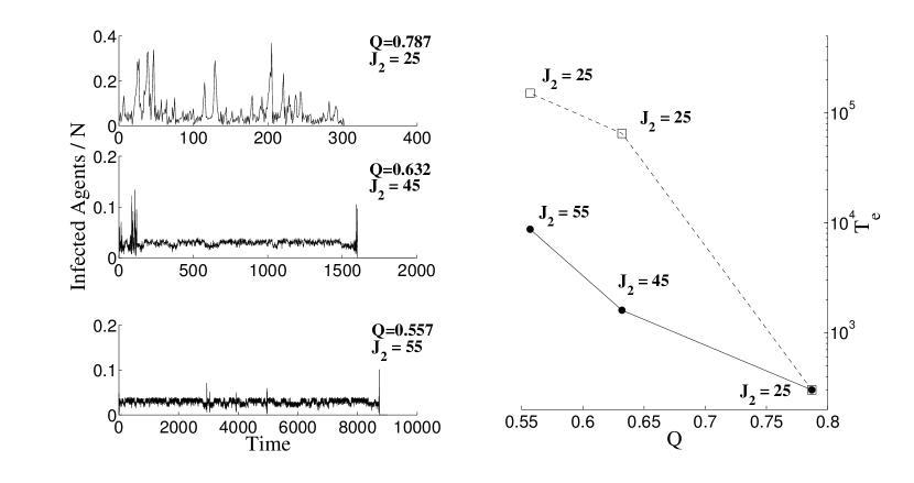
We studied the behavior of our model for different scenarios. In figure 5, we show results considering a network of $500$ nodes and $5$ communities where the initial number of infected agents is $\approx{}10\%$ of all agents in the network. We focus on the information about the community (parameter $J_{2}$), while we kept fixed $J=J_{1}=1$. It is very interesting to observe the time necessary for the extinction of the epidemics, with the probability of being infected $\tau=0.5$ and changing the community structure of the network.

On the left side of figure 5 we show the temporal evolution of the percentage of infectious agents for different kind of networks and different values of $J_{2}$. We can observe that the extinction time increases when the modularity of network decreases, even if we use higher values of $J_{2}$. On the right side of figure 5, we show the effect of the precaution on the extinction time. The straight line corresponds to different values of $J_{2}$, while the dotted line corresponds to the same value of $J_{2}$ in different kind of networks. It is also possible to observe that when a network becomes less clustered, the information about the community becomes less important.

In the case of scale-free networks, the mean connectivity degree $\left\langle k\right\rangle$ is related to the number $m$ of links the new nodes create. In the above example, considering $m=5$, we obtained a mean connectivity degree $\left\langle k\right\rangle=7.8$.

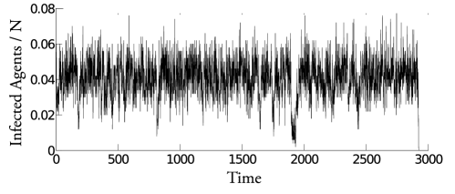
For comparisons, we generated random networks with a mean connectivity degree $\left\langle k\right\rangle\in(7,8)$. The first result that we obtained is that the extinction time is larger than in the scale-free case. In figure 6, we show the temporal evolution of the infected agents for a random network with modularity $Q=0.78$ considering $J_{2}=25$ as in the upper plot on the left side of figure 5. For the scale-free network the time necessary for the extinction is $T_{e}\simeq{}3\cdot 10^{2}$ while for the random one it is $T_{e}\simeq{}3\cdot 10^{3}$.

Figure 6: Percentage of infected agents for a random network of $100$ nodes and $5$ communities with modularity $Q=0.78$. Adopting the same parameter used for the simulation reported in figure 5, we show how the time for the extinction (approx. $2900$ units) of the epidemic is greater than for the scale-free case (i.e., upper plot on the left side of figure 5).

			Critical Values
$Q$ (modularity)	$J$		$J_{1}$		$J_{2}$
0.78	45		15		25
0.64	40		15		45
0.35	40		20		55

Table 1: Critical values for the extinction of the epidemic on case of scale-free networks of $500$ nodes and $5$ communities considering a maximum threshold time $T_{max}=1000$, necessary for the extinction of the epidemics.

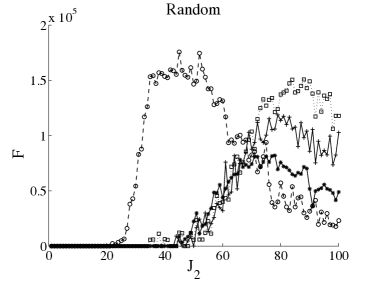
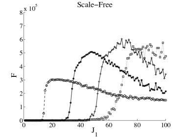
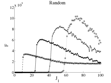
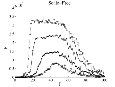
Regarding the effects of the global and local (neighborhood) information, we investigated scale-free networks composed by $500$ nodes and $5$ communities with a fixed maximum threshold time $T_{max}$, necessary for the extinction of the epidemics. We assume $T_{max}=1000$ and separately measure critical values of $J,J_{1}$ and $J_{2}$. In the table  1, we show the critical values of the three parameters by changing the modularity $Q$. As we can observe, the most variable parameter is $J_{2}$ while the other two parameters do not appear to change. From this figure, we observe that the information about the fraction of infected neighbors is the most effective for stopping the disease. However, in order to get this piece of information, each node needs to check the status of all its neighbours, a task that can be quite hard and possibly conflicting with privacy. On the other hand, the information on the average infectious level in the community or in the whole population is more easily obtained. Therefore, one needs to add the cost of information into the model in order to decide what the most effective solution for risk perception is.

Concluding, we have studied the progression and extinction of a disease in a SIS model over modular networks, formed by a certain number of random and scale-free communities. The infection probability is modulated by a risk perception term (modeling the probability of an encounter). This term depends on the global, local and community infection level. We found that in scale-free networks the progression is slower than in random ones with the same average connectivity. For what concerns the role of perception, we found that the local one (information about infected neighbours) is the most effective for stopping the spreading of the disease. However, it is also the piece of information that requires most efforts to be gathered, and therefore it may result a high cost/efficacy ratio.

A future direction of this work is an extension of the model by inserting a balance between the cost of information and the risk of being infected. In this regard, it should also be taken into account what the best strategies are to avoid the spreading of epidemics in different environments considering agents as intelligent entities capable to change or select the best strategies dynamically in order to minimize the risk and to maximize the economy of the system.

References

- [1] R. M. Anderson and R. M. May. Infectious Diseases of Humans Dynamics and Control. Oxford University Press, 1992.
- [2] F. Bagnoli, P. Liò, and L. Sguanci. Risk perception in epidemic modeling. Phys. Rev. E, 76:061904, Dec 2007.
- [3] A. L. Barabási and R. Albert. Emergence of scaling in random networks. Science, 286:509–512, 1999.
- [4] A. Barrat, M. Barthlemy, and A. Vespignani. Dynamical Processes on Complex Networks. Cambridge University Press, New York, NY, USA, 2008.
- [5] S. Boccaletti, V. Latora, Y. Moreno, M. Chavez, and D-U. Hwang. Complex networks : Structure and dynamics. Phys. Rep., 424(4-5):175–308, Fervier 2006.
- [6] M. Boguñá, R. Pastor-Satorras, and A. Vespignani. Absence of epidemic threshold in scale-free networks with degree correlations. Phys. Rev. Lett., 90:028701, Jan 2003.
- [7] J. Chen, H. Zhang, Z.-H. Guan, and T. Li. Epidemic spreading on networks with overlapping community structure. Physica A: Statistical Mechanics and its Applications, 391(4):1848 – 1854, 2012.
- [8] R. Cohen, D. ben Avraham, and S. Havlin. Percolation critical exponents in scale-free networks. Phys. Rev. E, 66:036113, Sep 2002.
- [9] Zoltán Dezső and Albert-László Barabási. Halting viruses in scale-free networks. Physical Review E, 65(5):055103+, May 2002.
- [10] S. Van Dongen. Graph clustering via a discrete uncoupling process. SIAM. J. Matrix Anal. and Appl., (30):121–141, 2009.
- [11] S. N. Dorogovtsev, J. F. F. Mendes, and A. N. Samukhin. Structure of growing networks with preferential linking. Phys. Rev. Lett., 85:4633–4636, Nov 2000.
- [12] C. Dorso and A.D. Medus. Community detection in networks. International Journal of Bifurcation and Chaos, 20(2):361–367, 2010.
- [13] S. Fortunato. Community detection in graphs. Physics Reports, 486(3-5):75 – 174, 2010.
- [14] S. Fortunato and C. Castellano. Community Structure in Graphs. December 2007.
- [15] M. Girvan and M. E. J. Newman. Community structure in social and biological networks. Proc. Natl. Acad. Sci., USA 99:7821–7826, 2002.
- [16] Stephan Kitchovitch and Pietro Liò. Risk perception and disease spread on social networks. Procedia Computer Science, 1(1):2339–2348, May 2010.
- [17] A. Lancichinetti, S. Fortunato, and J. Kertész. Detecting the overlapping and hierarchical community structure of complex networks. New Journal of Physics, 033015(11), 2009.
- [18] F. Liljeros, C. R. Edling, L. A. Amaral, E. H. Stanley, and Y. åberg. The web of human sexual contacts. Nature, 411(6840):907–908, June 2001.
- [19] C. Moore and M. E. J. Newman. Epidemics and percolation in small-world networks. Phys. Rev. E, 61:5678–5682, May 2000.
- [20] M. Newman. Networks: An Introduction. Oxford University Press, Inc., New York, NY, USA, 2010.
- [21] M.E.J. Newman. Detecting community structure in networks. Europ. Phys. J. B, (38):331–330, 2004.
- [22] M.E.J. Newman and M. Girvan. Finding and evaluating community structure in networks. Phys. Rev. E, (69):026113, 2004.
- [23] G. Palla, I. Derény, and T. Vickset. Nature, 435:814, 2005.
- [24] R. Pastor-Satorras and A. Vespignani. Epidemic dynamics and endemic states in complex networks. Phys. Rev. E, 63:066117, May 2001.
- [25] M. Salathé and J. H. Jones. Dynamics and control of diseases in networks with community structure. PLoS Comput Biol, 6(4):e1000736, 04 2010.
- [26] A. Saumell-Mendiola, M. A. Serrano, and M. Bogu ná. Epidemic spreading on interconnected networks. arXiv:1202.4087, 2012.