Emphasizing the different trends of the existing data for the $\gamma^{*}\gamma\to\pi^{0}$ transition form factor

Abstract

The new data on the $\gamma^{*}\gamma\!\!\to\!\!\pi^{0}$ transition form factor of the Belle Collaboration are analyzed in comparison with those of BaBar (including the older data of CELLO and CLEO) using an approach based on light-cone sum rules. Performing a 2-, and a 3-parametric fit to these data, we found that the Belle and the BaBar data have no overlap at the $1\sigma$ level. While the Belle data agree with our predictions, the Babar data are in conflict with them.

12.38.Lg, 12.38.Bx, 13.40.Gp, 11.10.Hi

1 Light-cone sum rules for the process $\mathbf{\gamma^{*}(Q^{2})\gamma(q^{2}\simeq 0)\to\pi^{0}}$

The validity of the collinear factorization — the basis of applications of QCD to hard processes — was challenged in the year 2009 by the experimental data measured by the BaBar Collaboration [1] for the kinematics $Q^{2}>m_{\rho}^{2},\ q^{2}\ll m_{\rho}^{2}$. This year, new experimental data by the Belle Collaboration [2] were presented that do not indicate such a growth and are grossly compatible with the QCD expectations. In this presentation, we show how these data and the previous ones by the CELLO [3] and CLEO [4] Collaborations can be analyzed within the theoretical scheme of light-cone sum rules (LCSR)s that incorporates contributions from QCD perturbation theory and higher-twist corrections. Within QCD, the pion-photon transition form factor (TFF) $F^{\gamma^{*}\gamma^{*}\pi^{0}}$ is given by the matrix element

$$\int\!d^{4}z\,e^{-iq_{1}\cdot z}\langle\pi^{0}(P)\mid T\{j_{\mu}(z)j_{\nu}(0)\}\mid 0\rangle=i\epsilon_{\mu\nu\alpha\beta}q_{1}^{\alpha}q_{2}^{\beta}F^{\gamma^{*}\gamma^{*}\pi^{0}}(Q^{2},q^{2})\ ,$$ (1)

where $j_{\mu}$ denotes the quark electromagnetic current and $Q^{2}\equiv-q_{1}^{2}>0$, $q^{2}\equiv-q_{2}^{2}\geq 0$. For the asymmetric kinematics $q^{2}<m_{\rho}^{2}$, one has to include into the calculation the interaction of the (quasi) real photon at long distances $\sim O(1/\sqrt{q^{2}})$. To accomplish this goal, we apply the approach of LCSRs [5, 6] that effectively accounts for the effects of the long-distance interactions of the real photon by making use of a dispersion relation in $q^{2}$ and applying quark-hadron duality in the vector channel [7, 8]. Taking the limit $q^{2}\rightarrow 0$, we get [6]

$$Q^{2}F^{\gamma^{*}\gamma\pi^{0}}\left(Q^{2}\right)=\!\!\!\!\! \frac{\sqrt{2}}{3}f_{\pi}\left[\frac{Q^{2}}{m_{\rho}^{2}}\int_{x_{0}}^{1}\exp\left(\frac{m_{\rho}^{2}-Q^{2}\bar{x}/x}{M^{2}}\right)\bar{\rho}(Q^{2},x)\frac{dx}{x}\right.$$ (2)

$$\left.+\int_{0}^{x_{0}}\!\!\bar{\rho}(Q^{2},x)\frac{dx}{\bar{x}}\right]\,,$$

where $M^{2}$ is the Borel parameter in the interval 0.7-0.9 GeV² and the spectral density is given by $\bar{\rho}(Q^{2},x)=(Q^{2}+s)\rho^{\text{pert}}(Q^{2},s)$ with

$$\rho^{\text{pert}}(Q^{2},s)=\frac{1}{\pi}{\rm Im}F^{\gamma^{*}\gamma^{*}\pi^{0}}\left(Q^{2},-s-i\varepsilon\right)=\rho_{\text{tw-2}}+\rho_{\text{tw-4}}+\rho_{\text{tw-6}}+\ldots\,.$$ (3)

The various twist contributions are defined in the form of convolutions of the corresponding hard parts with the pion distribution amplitude (DA) of a given twist [6]. For instance, for the twist-four contribution we use the effective description [6] $\varphi_{\pi}^{(4)}(x,\mu^{2})\sim\delta_{\text{tw-4}}^{2}(\mu^{2})\,x^{2}(1-x)^{2}$ with $\delta_{\text{tw-4}}^{2}(\mu^{2})=0.19\pm 0.04$ GeV² [7]. Here we used the abbreviations $\bar{x}=1-x$, $s=\bar{x}Q^{2}/x$, $x_{0}=Q^{2}/(Q^{2}+s_{0})$, where $s_{0}\simeq 1.5~{}\text{GeV}^{2}$ is the effective threshold in the vector channel. The leading twist-two contribution has the perturbative expansion ($a_{s}=\alpha_{s}/(4\pi)$)

$$F_{\gamma^{*}\gamma^{*}\pi^{0}}^{\text{tw-2}}\sim(T_{\text{LO}}+a_{s}(\mu^{2})T_{\text{NLO}}+a_{s}^{2}(\mu^{2})T_{\text{NNLO}_{\beta_{0}}}+\ldots)\otimes\varphi_{\pi}(x,\mu^{2})\,.$$ (4)

The corresponding contributions from (4) to the spectral density (3) have been obtained in [9]. For the term $\rho_{\rm NLO}$ we employ the corrected version computed in [10]. The “bunch” of the admissible twist-two pion DAs $\varphi_{\pi}(x,\mu^{2})$ was determined in [11] within the framework of QCD SRs with nonlocal condensates (NLC)s. This DA “bunch” (shown graphically in Fig. 1 in the form of a rectangle) can be effectively parameterized in terms of the first two Gegenbauer coefficients $a_{2}$ and $a_{4}$ to reduce the expansion to $\varphi_{\pi}^{\rm BMS}(x)=6x\bar{x}\left[1+a_{2}C_{2}^{3/2}(2x-1)+a_{4}C_{4}^{3/2}(2x-1)\right].$ Our next goal is to extract a pion DA that provides best agreement with all sets of the existing data by performing a fit procedure of the Gegenbauer coefficients $a_{n}$ within the basis of LCSRs, cf. Eq. (2). The results for the combined set of data from CELLO&CLEO&Belle – termed CCBe — will be contrasted to those from the CELLO&CLEO&BaBar set — called CCBB.

2 2D-analysis of the combined data fit

In Fig. 1, we present the confidence region of the $a_{2},a_{4}$ values in the form of error ellipses in the $(a_{2},a_{4})$ plane, obtained by fitting different sets of data. We take into account only statistical errors and exclude theoretical uncertainties — in contrast to our previous work in [7, 8]. Using LCSRs with the pion DAs obtained in QCD SR NLC [11], one arrives at the predictions shown in terms of the (green) rectangle in comparison with the error ellipses pertaining to the different sets of data defined in the previous section.

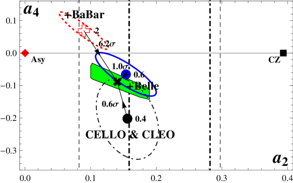
Figure 1: Error ellipses of various sets of data described in Sec. 1 and taken at $\mu=2.4$ GeV scale. The best-fit values of $\chi^{2}$ are shown at the centers of the ellipses, while differences between data sets are displayed along the links in units of 1$\sigma$. The vertical lines show the range of values computed on the lattice: dashed line—[12]; dashed-dotted line—[13].

The best-fit values of the $\chi^{2}$ goodness criterion $\chi^{2}_{\text{ndf}}\equiv\chi^{2}/\text{ndf}$ (ndf=number of degrees of freedom) are shown as centers of the ellipses, with the deviations from one data set to another with reference to the rectangle being displayed along the links and expressed in units of one standard deviation (1$\sigma\approx 68\%$). We conclude that the inclusion of the BaBar data to those obtained before by CELLO&CLEO leads to an approximately 3$\sigma$ shift [14] of the confidence region away from the (black) ellipse at the bottom. The result is represented by the (red) dotted ellipse at the top accompanied by a significant increase of $\chi^{2}_{\text{ndf}}$ from 0.4 to 2 (for the CCBB data set). If we include to the CELLO&CLEO data only the Belle data set CCBe, then the shift of the confidence region is only moderate giving rise to a slight increase of $\chi^{2}_{\text{ndf}}$ from 0.4 to 0.6 (ellipse in the middle). We quantify the deviations of these data sets from our theoretical estimates, encoded in the rectangle, in terms of $\sigma$ values shown along the links which connect the central data values with the BMS model (✖) inside the rectangle. Here, and in the next figure, the vertical broken lines denote the constraints from two different lattice simulations: dashed lines — [12]; dashed–dotted lines — [13].

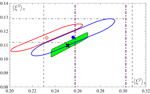
Figure 2: (color online). Predictions for the moments $\langle\xi^{2}\rangle$ and $\langle\xi^{4}\rangle_{\pi}$ at the lattice scale $\mu^{2}_{\text{Lat}}=4$ GeV². The lower stretched ellipse — solid (blue) line — corresponds to a 2D fit to the CCBe data, while the upper one (red line) represents the CCBB one. In contrast to Fig. 1, we also include here the uncertainty related to the twist-four coefficient $\delta^{2}_{\text{tw-4}}$. The vertical lines show the range of values computed in two lattice calculations using the same designations as in Fig. 1.

An immediate conclusion from these considerations is that (i) the BMS DA is inside the 1$\sigma$ CCBe and inside the 0.6$\sigma$ region of the CELLO&CLEO set, whereas the BMS “bunch” greatly overlaps with both of these error ellipses. At the same time, the central point of CCBB is 6.2$\sigma$ away and has no overlap with the CCBe ellipse. (ii) The asymptotic DA (◆) and the Chernyak-Zhitnitsky (CZ) DA (◼) are both more than $6\sigma$ away from CCBe. (iii) The existing lattice calculations of $a_{2}$, shown as vertical lines in Figs. 1,2, are not restrictive enough to narrow down the interval of $a_{2}$, though the narrower band [13] supports both the CCBe data and our theoretical results but not the CCBB data. On the other hand, the previous lattice simulation [12] is compatible with all sets of data and with our theoretical predictions as well.

With all these data in our hands, we may attempt to extract values of the moment $\langle\xi^{4}\rangle_{\pi}$ by combining the real data from CCBe and CCBB with the results of lattice simulations. The combined constraints from CCBe (lower (blue) error ellipse in Fig. 2) and the lattice constraints from [13] (dashed-dotted vertical lines) lead to the following predictions for $\langle\xi^{4}\rangle_{\pi}$: $\langle\xi^{2}\rangle_{\pi}\in[0.26\div 0.30]$ and $\langle\xi^{4}\rangle_{\pi}\in[0.112\div 0.13]$. In contrast, the constraints extracted from the CCBB data (upper (red) ellipse) do not allow a reliable determination of the $\langle\xi^{4}\rangle_{\pi}$ range in the background of the lattice results from [13]. On the other hand, the constraints from [12] are not stringent enough to differentiate these sets of data.

3 3D-analysis of the combined data

We step up from a 2D to a 3D analysis of the data, by including the next coefficient $a_{6}$. Then, we get in Fig. 3 fit results in terms of $1\sigma$ ellipsoids with respect to the experimental statistical errors for the CCBe data set (left panel) and the CCBB (right panel). The theoretical $\mp\Delta\delta^{2}_{\text{tw-4}}$-error is indicated by a solid (red) cross for an increasing value of $\delta^{2}_{\text{tw-4}}$, whereas a dashed (green) cross (closer to the $a_{6}$ axis) denotes a decreasing value.

 

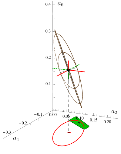
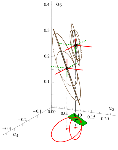
Figure 3: 3D graphics of the $1\sigma$ error ellipsoids in the space spanned by the Gegenbauer coefficients $a_{n}$ $(n=2,4,6)$ for processing the data on the pion-photon transition form factor within the LCSR approach using the scale $\mu$=2.4 GeV. Left. Only CCBe data used. Right. CCBB fit (smaller ellipsoid) shown in comparison with CCBe data. More explanations are given in the text.

The projection of the CCBe $1\sigma$ ellipsoid on the plane $(a_{2},a_{4})$ is represented, in both panels, by the larger (red) ellipse, while the smaller one refers to CCBB. The shaded (green) rectangle encloses the region of $a_{2},a_{4}$ pairs allowed by NLC SRs [11], with the symbol (✖) marking the BMS pion DA. All results are shown at the scale $\mu=2.4$ GeV after NLO evolution.

To further quantify these statements, we supply the “coordinates” of the central point of each of the two displayed ellipsoids in the following form. The first number gives the central value of the fit, the next number is the statistical 1$\sigma$ error, and the third one is the theoretical uncertainty due to twist-four. Then, we have: CCBe $(0.157\pm 0.057\pm 0.056,-0.192\pm 0.122\pm 0.077,0.226\pm 0.161\pm 0.033)$ with  $\chi^{2}_{\text{ndf}}=13.1/30$; CCBB $(0.177\pm 0.054\pm 0.056,-0.171\pm 0.103\pm 0.071,0.307\pm 0.096\pm 0.024)$ with  $\chi^{2}_{\text{ndf}}=33.3/32$.
To conclude: (i) The description of the CCBe data provides a better $\chi^{2}_{\text{ndf}}\approx 0.4$ relative to $\chi^{2}_{\text{ndf}}\geq 1$ following from CCBB. (ii) The CCBe and CCBB ellipsoids are significantly separated from each other, so that a QCD description of these sets of data requires substantially different DAs. (iii) The $(a_{2},a_{4})$ projections of both ellipsoids have a good overlap with the BMS “bunch”, though the CCBe ellipsoid that has no intersection with it. An intersection is possible but only at a larger value of confidence level.

4 Local characteristics of the pion DA

The confidence region of the coefficients $\{a_{n}\}$, obtained in Sec. 3, can be linked to other characteristics of the pion DA. The profiles of the pion DA $\varphi_{\pi}(x)$, extracted in the 3D fit procedure, are shown in Fig. 4: left panel — set CCBe; right panel — set CCBB. The BMS “bunch” (shaded green strip) and the BMS DA model (black solid line inside it) are also shown.

  

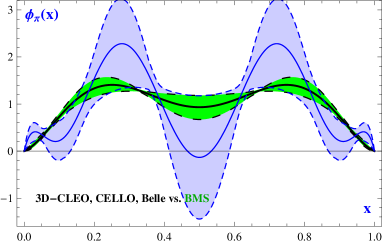
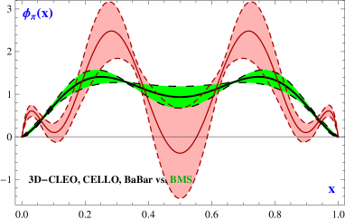
Figure 4: Left. Comparison of the BMS pion DA “bunch” (darker shaded strip in green) and of the BMS model (black solid line inside this strip) with the 3D fit to the experimental data on the pion-photon transition form factor. The solid blue line denotes the best-fit pion DA (at the scale $\mu=2.4$ GeV, see second paper in [6]) obtained from the analysis of the set CCBe, with the dashed lines indicating the sum of the statistical errors of the fit and the twist-four uncertainties. Right. Analogous results obtained with the set CCBB.

The main difference between the two graphics in Fig. 4 stems from their distinct behavior near the endpoints that are concentrated inside the interval $\Delta=0.05$. Indeed, one observes that the DA (including uncertainties) — shaded area in the right panel — providing best-fit to the CCBB data deviates significantly from the BMS “bunch”. A mathematical tool to quantify the endpoint characteristics of the pion DA is $D^{(m)}\varphi(\Delta)$, i.e., the average derivative of $\varphi(x)$ in the interval $\Delta$, that was invented in [15] and possesses the following properties: $\lim\limits_{\Delta\to 0}D^{(m)}\varphi_{\pi}(0)(\Delta)=\varphi^{\prime}_{\pi}(0);\lim\limits_{m\to\infty}D^{(m)}\varphi_{\pi}(0)(\Delta)=\varphi^{\prime}_{\pi}(0)$, while $D^{(2)}\varphi(1)=\int_{0}^{1}dx\varphi_{\pi}(x)/x$. The quantity $D^{(2)}\varphi(\Delta)$ can be used [16] to probe the endpoint behavior of these different sorts of DAs:

$$D^{(2)}\varphi(0.05)=17.2\pm 8.5~{}\text{ for CCBe};~{}25.6\pm 5.25~{}\text{for CCBB}\,.$$ (5)

We see that the slope in the endpoint region of the best-fit DA to CCBB is much stronger than for CCBe. While the CCBe-based DA profile agrees with the BMS “bunch”, it is incompatible with the CCBB shape.

5 Conclusions

We presented here an analysis of all experimental data on the pion-photon transition form factor and compared in detail the results obtained with two different sets of data: CELLO, CLEO, BaBar — (CCBB) vs. CELLO, CLEO, and Belle — (CCBe). Our analysis is based on LCSRs at NLO, also taking into account the twist-four term. The NNLO_β radiative correction was included into the theoretical uncertainties together with the twist-six contribution [10]. The key results can be summarized as follows: (i) We performed a 2D (parameters $a_{2},a_{4}$) and a 3D (parameters $a_{2},a_{4},a_{6}$) analysis, fitting both the CCBe and the CCBB data sets. We found that in both cases the fit to CCBe provides a significantly better $\chi^{2}_{\text{ndf}}$ value. (ii) The CCBe 2D fit agrees well within error bars with the previous findings from the CELLO and CLEO fits and the predictions derived from QCD SR NLC[11] with the BMS “bunch” and the BMS model DA. The fits are also compatible with the constraints on $a_{2}$ extracted from lattice computations. In contrast, the CCBB 2D fit has no overlap with the CCBe result and it also does not comply with the QCD SR NLC predictions. (iii) The results of the 3D fit to the CCBe and CCBB data sets do not intersect at the level of a 1$\sigma$ accuracy. At the same time the CCBe result is much closer to the BMS “bunch”, but still outside the 1$\sigma$ area. (iv) The qualitative features of the 3D fit to the CCBe and CCBB data can be differentiated in terms of the behavior of the corresponding profiles of the pion DAs near the endpoints: the CCBe has a less pronounced slope and is close to the BMS “bunch”, whereas the slope of CCBB is larger and gives no support to the BMS DAs.

We acknowledge support from the Heisenberg-Landau Program (Grant 2012), Russian Foundation for Fundamental Research (Grant No. 12-02-00613a), and the BRFBR JINR Cooperation Program (contract No. F10D-002). The work of A.V.P. was supported in part by HadronPhysics2, Spanish Ministerio de Economia y Competitividad, and EU FEDER under contracts FPA2010-21750-C02-01, AIC10-D-000598, GVPrometeo2009/129.

References

- [1] B. Aubert et al., Phys. Rev. D80, 052002 (2009).
- [2] S. Uehara et al., Phys. Rev. D86, 092007 (2012).
- [3] H.J. Behrend et al., Z. Phys. C49, 401 (1991).
- [4] J. Gronberg et al., Phys. Rev. D57, 33 (1998).
- [5] I.I. Balitsky, V.M. Braun, A.V. Kolesnichenko, Nucl. Phys. B312, 509 (1989).
- [6] A. Khodjamirian, Eur. Phys. J. C6, 477 (1999); A. Schmedding, O. Yakovlev, Phys. Rev. D62, 116002 (2000).
- [7] A.P. Bakulev, S.V. Mikhailov, N.G. Stefanis, Phys. Rev. D67, 074012 (2003).
- [8] A.P. Bakulev, S.V. Mikhailov, A.V. Pimikov, N.G. Stefanis, Phys. Rev. D84, 034014 (2011); Phys. Rev. D86, 031501(R) (2012).
- [9] S.V. Mikhailov, N.G. Stefanis, Nucl. Phys. B821, 291 (2009); corrected in arXiv:0905.4004v6.
- [10] S.S. Agaev, V.M. Braun, N. Offen, F.A. Porkert, Phys. Rev. D83, 054020 (2011); Phys. Rev. D86, 077504 (2012).
- [11] A.P. Bakulev, S.V. Mikhailov, N.G. Stefanis, Phys. Lett. B508, 279 (2001); Erratum: ibid. B590, 309 (2004).
- [12] V.M. Braun et al., Phys. Rev. D74, 074501 (2006).
- [13] R. Arthur et al., Phys. Rev. D83, 074505 (2011).
- [14] A.V. Pimikov, A.P. Bakulev, S.V. Mikhailov, N.G. Stefanis, AIP Conf. Proc. 1492, 134 (2012).
- [15] S.V. Mikhailov, A.V. Pimikov, N.G. Stefanis, Phys. Rev. D82, 054020 (2010).
- [16] A.P. Bakulev, S.V. Mikhailov, A.V. Pimikov, N.G. Stefanis, Nucl. Phys. B (Proc. Suppl.) 219-220, 133 (2011).