Selectable linear or quadratic coupling in an optomechanical system
Abstract
There has been much interest recently in the analysis of optomechanical systems incorporating dielectric nano- or microspheres inside a cavity field. We analyse here the situation when one of the mirrors of the cavity itself is also allowed to move. We reveal that the interplay between the two oscillators yields a cross-coupling that results in, e.g., appreciable cooling and squeezing of the motion of the sphere, despite its nominal quadratic coupling. We also discuss a simple modification that would allow this cross-coupling to be removed at will, thereby yielding a purely quadratic coupling for the sphere.
Several early optomechanical systems Arcizet et al. (2006); Gigan et al. (2006); Gröblacher et al. (2009a) were straightforward realisations of ideas first proposed by Braginsky and Manukin Braginsky and Manukin (1967, 1977), and took the form of a Fabry–Pérot cavity with one moving mirror. These systems are naturally modelled by the Hamiltonian Wilson-Rae et al. (2007); Marquardt et al. (2007) (we will use units such that throughout this paper) , where we have introduced the term
| (1) |
with the annihilation operator representing the cavity field (frequency ), [] the position [momentum] operator for the moving mirror (frequency and mass ), and the optomechanical coupling constant. Physically, admits a remarkably simple interpretation: the instantaneous position of the mirror changes the length of the cavity, and thus its resonance frequency.
The light–mirror interaction inherent in Eq. (1) enables the passive cooling of the mechanical system, an effect that has been demonstrated in a vast array of experimental settings Arcizet et al. (2006); Gigan et al. (2006); Schliesser et al. (2006); Kleckner and Bouwmeester (2006); Corbitt et al. (2007) and that has been progressively pushed to the point that optical cooling to the mechanical quantum ground state was recently achieved Chan et al. (2011). Moreover, it has long been recognised that the mechanical and optical fields can be prepared in an entangled steady-state Vitali et al. (2007); Paternostro et al. (2007) by the means of Eq. (1). Bhattacharya and Meystre Bhattacharya and Meystre (2007) proposed a different paradigm, where the moving mirror was translucent and placed inside the cavity, a configuration that was implemented in the seminal experiment reported in Refs. Thompson et al. (2008); Sankey et al. (2010). A remarkable feature of this model is that, under the right conditions and differently from the above, the light–mirror interaction may be described through an optomechanical Hamiltonian quadratic in the position operator of the mechanical system and reading
| (2) |
where is a coupling constant. This model has several interesting properties, including the possibility of performing QND measurements of the occupation number of the oscillator Clerk et al. (2010), but precludes cooling to leading order in the linearised regime achieved when the cavity field is populated by a very large number of photons Bhattacharya et al. (2008) (see, however, Ref. Nunnenkamp et al. (2010) for a treatment that goes beyond the linearised dynamics of the system).

In this paper we propose to combine these two scenarios, somewhat in the spirit of proposals that place a cloud of ultracold atoms inside an optomechanical setup Paternostro et al. (2010); De Chiara et al. (2011); Rogers et al. (2012). Let us consider the system shown in Fig. 1, which includes a small dielectric scatterer (herein referred to as the sphere) held in a harmonic potential inside a cavity Chang et al. (2009); Romero-Isart et al. (2010, 2011a, 2011b); Romero-Isart (2011); Li et al. (2011); Monteiro et al. (2012), one of whose end-mirrors is allowed to oscillate. As we shall show, this system allows us to exert a degree of control on the state of the motion of the sphere through its indirect interaction with the end-mirror, mediated by the cavity field. As a result of this, and by means of a judicious choice of operating parameters, we will show that passive cooling of the motion of the sphere, despite its apparent quadratic coupling to the cavity field, and squeezing of this same motion are both possible. Moreover, we expect that the interaction between the cavity field, sphere, and end-mirror gives rise to steady states with interesting genuinely tripartite entangled Xuereb et al. (2012) or nonlocal Lee et al. (2012) properties.
One might think that the Hamiltonian that describes this compound system would simply be given by the sum of the interaction terms in through the position of the end-mirror and through the position of the sphere. As natural as this might seem, this would not be entirely correct, given that the position of the end-mirror not only defines the resonance frequency of the cavity (as captured through the interaction in ), but also determines the relative position of the cavity field (anti)nodes and the sphere. This means that, for the configuration shown in Fig. 1, i.e., for a cavity pumped from the leftmost (fixed) mirror, the light field couples quadratically to the relative position operator . We can thus write the Hamiltonian
| (3) |
where the subscript ‘lp’ reminds us that the system is pumped from the left. In Appendix A, we examine the other possibilities for the geometry of the pump field.
The remainder of this paper is structured as follows. Section I will set the stage for exploring the dynamics of our system, deriving in particular the Hamiltonian and the linearised equations of motion. Section II subsequently makes use of numerical simulations to discuss the resulting dynamics. As an application of our scheme, we show that the cross-coupling between the two oscillators, cf. Eq. (3), gives rise to efficient cooling of the mechanical motion of the sphere. In Sec. III we discuss squeezing of the motion of the sphere and demonstrate that this motion can be squeezed appreciably if the coupling constant is large enough. Finally, we conclude with an outlook of possible future directions.
I Dynamics in the linearised regime
Let us start by considering the model in Fig. 1. Classically, the intensity of the field within the cavity at a distance from the right mirror is given by , where the depends on the value of the wavenumber and the amplitude of the input field. To treat our oscillators quantum-mechanically we perform the replacement
| (4) |
where is the distance between the equilibrium positions of the two oscillators. Let us choose such that , with the wavelength of the input light. With this choice, the sphere oscillates about a node or an antinode of the cavity field. The interaction Hamiltonian involving the sphere thus takes the form
| (5) |
We now expand Eq. (5) as a series, stopping at the lowest order, introduce dimensionless mechanical operators [obtained by dividing out the extent of the zero-point fluctuations of each oscillator, where is the mass and the oscillation frequency of the mirror () or the sphere ()], and add back the linear optomechanical coupling between and . This gives us the total interaction Hamiltonian
| (6) |
where, as before, and are optomechanical coupling constants and . The signs in front of the coupling constants are chosen to aid interpretation: the system shown in Fig. 1 has positive , and implies that the sphere oscillates about an antinode, i.e., a point of stable equilibrium. A full description of the system requires also the free Hamiltonian, which we write in a frame rotating at the frequency of the driving laser ,
| (7) |
as well as cavity-pump () and dissipation Hamiltonians (), which will be left unspecified. Here, is the cavity–pump detuning. The full Hamiltonian is thus . The corresponding equation of motion for the cavity field operator is
| (8) |
where is the cavity amplitude decay rate, and is the input field. As for the sphere and mechanical mode, the dynamics is encompassed by
| (9) | ||||
where , are the mechanical decay rates, and is the self-adjoint zero-mean operator describing the Brownian noise affecting oscillator and characterised by the correlation functions Giovannetti and Vitali (2001)
| (10) |
where is the equilibrium phononic population of oscillator at temperature ( is the Boltzmann constant).
I.1 Classical steady-state solution
Equations (9) are tackled in two steps. First we replace each operator by its quantum-mechanical mean value . The resulting equations of motion are identical to the classical ones. Their solution is then used in a second step, as described in Sec. I.2, to analyse the linear evolution of the system. We remark here that , and that relates to the input power as . When the dynamics is stable, the long-time classical solutions are
| (11) |
where we have replaced the detuning with and introduced the quantities
| (12) | ||||
Equations (11) diverge in a notable way from the analogous ones reported in Ref. Bhattacharya et al. (2008). The latter case corresponds to ours upon going to the infinite-mass limit for the end-mirror (). From Eqs. (11) it then follows that . An immediate consequence of this is that in the linearised equations of motion, as obtained in the next Section, the motion of the mirror is decoupled from the rest of the system [cf. Eq. (18)]. Under these conditions, therefore, the effective mechanical decay rate of the sphere cannot be altered by the dynamics in the linear approximation, i.e., the motion of the sphere cannot be cooled by a quadratic interaction with the cavity field. Outside the infinite-mass limit, however, the two oscillators interact to avoid this pitfall. As we shall see later on, one can choose the parameters such that cooling of the sphere to a temperature determined mostly by the properties of the end-mirror is indeed possible, thus demonstrating the control mechanism at the centre of our work.
I.2 Linearised equations of motion
Having at hand the explicit form of the operators’ mean values, we now consider the zero-mean quantum fluctuations . When one can truncate the equations of motion to first order in the fluctuations, yielding the set of linear equations of motion
| (13) |
Here, we have defined the vectors of quadrature fluctuations , where and , as well as with and that are defined analogously to and . The input noise field obeys and . Moreover, we have introduced the drift matrix , whose (lengthy) expression is given in Appendix B. Stability of the dynamics encompassed by Eq. (13) is easily studied by using the well-known Routh–Hurwitz criterion (Horn and Johnson, 1994, §2.3.2), which (in its most straightforward formulation) guarantees the existence of a stable solution if all of the eigenvalues of have negative real part. All of the following analysis is conducted in this stable regime.
The linearised dynamics for the operator increments can be derived from a quadratic effective Hamiltonian. For a fixed set of parameters, the dynamics therefore leads any initial Gaussian state to a unique final Gaussian steady state. This steady state has zero first moment, since we operate in a shifted picture involving only zero-mean operator increments, and the matrix of second moments satisfies the Lyapunov equation , where
We remark that the Lyapunov equation admits a compact solution in in terms of the eigensystem of (Horn and Johnson, 1994, §5.0.4). Having at hand the covariance matrix , we can readily analyse the (Gaussian) steady state of the system, including bipartite entanglement between any two components of the system, genuine tripartite entanglement, or occupation numbers for the two harmonic oscillators.
(a)
(b)
II Cooling of the sphere
In this Section, we shall demonstrate the claimed cooling mechanism for the trapped sphere, and the control we can operate on it through the means of the mechanical mirror. Before specifying the values of the various parameters that enter our dynamical equations, let us give explicit formulae for and . The basic theory of cavity optomechanics identifies with the first-order change in the cavity resonance frequency when the end-mirror moves by a distance Kippenberg and Vahala (2007). For a cavity of length we can thus write Xuereb and Domokos (2012)
| (14) |
For , in the case of spheres that are not too large, we use the expression in Ref. Romero-Isart (2011)
| (15) |
where is the volume of the sphere, is the mode volume for a cavity with waist , is the wavenumber of the driving field, and its wavelength. The sign of this expression is chosen depending on whether the sphere is at a node () or an antinode () of the cavity field. In the case of a lossless dielectric of real refractive index , , and we can write this expression as
| (16) |
where is the mass density of the material composing the sphere. Note, in particular, that is independent of the radius of the sphere. For silica kg m-3 and, in the near infrared, . We shall use nm, cm, kHz, m, m (which can all be found in Ref. Monteiro et al. (2012)), and ng Gröblacher et al. (2009b). For the mechanical damping constants, we take the values Hz Gröblacher et al. (2009a) and mHz. At the two nominal frequencies MHz and kHz, we find Hz, Hz at a node of the cavity field, and . In what follows we will not constrain ourselves to these particular values of , however, and will scale and appropriately. In passing, we note that and can be made larger by decreasing the length of the cavity or lowering the mechanical oscillation frequencies. Moreover, can be increased by lowering the effective mass of the moving mirror, while by using a sphere with a larger refractive index or a cavity with a smaller waist. Finally, the value of can be made larger by increasing the ratios and .
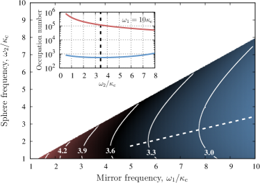
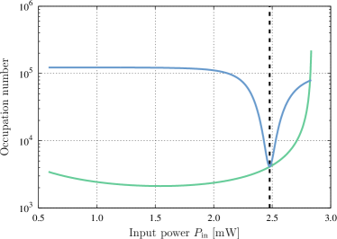
We have already mentioned how gives rise to the steady-state solution Bhattacharya et al. (2008). In the linearised regime, the motion of the sphere is thus decoupled from that of the dynamics of the cavity–mirror system. This can easily be seen by substituting and into the drift matrix . A straightforward method to explore the implications of the coupling induced by our interaction Hamiltonian is thus to look at cooling of the motion of the sphere. A sample of such data is shown in Fig. 2. The cases (i) or (ii) have been excluded from the plot for reasons that will be clarified later on. We see that, for each , there exists a band of frequencies for which the steady-state occupation for the spherical motion is significantly below the starting value. Moreover, for a particular that depends most strongly on the properties of the mirror (in particular, the constant parameter ), the motion of the mirror and sphere equilibrate to the same occupation number. The data displayed in Fig. 2 show the reduction of the occupation number of the sphere by almost three orders of magnitude. However, in our numerical exploration we have seen evidence that this is not an upper limit to the efficiency of the process. Indeed, decreasing the temperature of the thermal bath to which the mirror is coupled will yield a correspondingly lower occupation number for the sphere, as a result of dynamical equilibration of the sphere through the mechanical mirror.
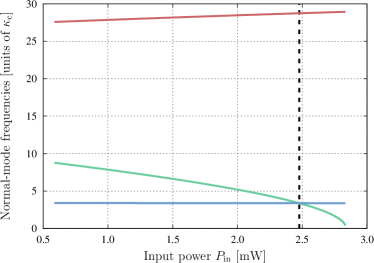
The basic mechanism through which this cooling process occurs is a hybridisation of the motion of the two oscillators. For moderately large values of , increasing the input power from zero causes the frequencies of the normal modes of the system, given by the imaginary parts of the eigenvalues of , to shift. Thus, for instance, the mode that at describes the mirror motion shifts to a smaller frequency Genes et al. (2008). At the point where , the two modes hybridise and cooling ensues. For , this hybridisation is no longer possible. However, if is too large, the system reaches instability before the criterion can be satisfied. Conversely, if is not large enough, the power at which is satisfied is too low for efficient cooling. Such hybridisation can be seen in Fig. 3, where we plot the case , at the optimal values for and .
Another unique feature of our system is that, after cooling the sphere, we can switch to coupling light into the cavity from the moving mirror. As explained in Appendix A, this means that the Hamiltonian that couples the motion of the sphere to the optical field is purely quadratic. This renders possible, for example, quantum non-demolition (QND) measurements of the energy of the harmonic oscillator embodied by the sphere. This protocol requires that the cavity can be pumped from either end-mirror, but is deterministic and otherwise less demanding than, e.g., measurement-based schemes for achieving the same Vanner (2011).
(a)
(b)
III Squeezing of mechanical motion
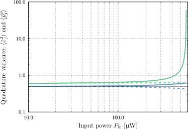
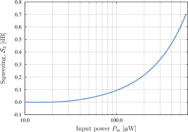
The coupling of mechanical elements to a light field, both linearly Mancini and Tombesi (1994) and quadratically Nunnenkamp et al. (2010), can give rise to squeezing of the mechanical motion, where the quantum nature of the optomechanical interaction acts to suppress the noise in one of the quadratures of the mechanical motion. To investigate the occurrence of mechanical squeezing in our setup we set the temperature of the baths coupled to both oscillators to zero. For the parameters given above, there is no observable squeezing in the motion of the sphere, and to induce such effects we have found it necessary to use a larger value for , e.g., two orders of magnitude larger in the case of the data presented in Fig. 4.
To quantify the amount of squeezing in the steady state of the linearised dynamics, we used the figure of merit
| (17) |
as plotted in Fig. 4(b) for . In other words, only when the variance of one of the quadratures dips below the -quantum level that is due to vacuum fluctuations in the ground state. We find a maximal dB () just before the instability threshold, which compares favourably to the amount of squeezing obtained in Ref. Nunnenkamp et al. (2010) for pure quadratic coupling.
We conclude this Section by noting that the larger quadratic coupling strengths necessary for generating and observing squeezing can be obtained by making use of avoided crossings between pairs of cavity modes Sankey et al. (2010).
IV Conclusions
We have explored a system consisting of an optomechanical cavity with an additional intra-cavity particle whose motion is coupled quadratically to the cavity field. A direct coupling between the two moving elements arises naturally in this system. This coupling can be turned off and on at will by choosing which port the cavity is driven from, and therefore provides complete control over whether the interaction with the particle is purely quadratic, or whether it has some linear character. As examples of the potential of our scheme, we have discussed the possibility of cooling the motion of the sphere, despite its nominal quadratic coupling, as well as squeezing of this same motion. Our work opens up interesting perspectives for quantum state-transfer between two oscillators and the distribution of multipartite entanglement. Moreover, the system that we have addressed leaves room for asking interesting questions on the nonlocal nature of the three-mode state achieved via the coupling mechanisms addressed here, a goal that can be pursued, for instance, through the formal apparatus recently put forward in Ref. Lee et al. (2012).
Acknowledgements
AX thanks the University of Malta for hospitality during completion of this work and the Royal Commission for the Exhibition of 1851 for financial support. MP is supported by the UK EPSRC through a Career Acceleration Fellowship and the “New Directions for EPSRC Research Leaders” initiative (EP/G004759/1). Parts of the calculations were carried out using computational facilities funded by the European Regional Development Fund, Project ERDF-080.
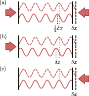
Appendix A Alternative pumping geometries
The function of this Appendix is to elucidate the differences between pumping the cavity from the immobile mirror, from the moving mirror, or from both ends. These three possibilities, which are exhaustive in one-dimensional geometries, are illustrated in Fig. 5. The geometry used throughout this paper is shown in Fig. 5(b). The most ‘natural’ case, where the cavity field is symmetric with respect to coordinate inversion, is depicted in Fig. 5(a). In both these situations, when the mirror on the right moves, the nodal structure shifts with respect to the laboratory frame, yielding a term in the Hamiltonian that couples the two oscillators. In the case of Fig. 5(c), however, the nodes of the field do not shift when the mirror moves, such that there is no longer any cross-coupling between the two oscillators. The case of a resonant cavity pumped from one end is special: since all the input light is transmitted and none is reflected off the cavity, both mirrors effectively interact with three running waves of nonzero amplitude, two moving away from the pump, one towards it, such that the right mirror is a time-reversed copy of the left mirror. The entire system is therefore invariant under inversion of coordinates and time reversal.
In our notation, the part of the interaction Hamiltonian that involves the sphere can be represented as
with reference to the respective cases in Fig. 5. The main text can be adapted for the remaining cases by setting [case (a)] or [case (c)].
This interesting result can easily be seen for case (b) (and analogously for the other two cases) by calculating the field inside the cavity, normalised to the input field, at a distance from the right mirror. That is
where is the length of the cavity, the wavenumber of the field, accounts for the spectral profile of the resonance, and depends only on the distance from the right mirror. For simplicity, the two mirrors are assumed to be identical, with (real) reflectivity and transmissivity , and any phase shifts upon reflection or transmission are absorbed in ; these simplifications are not crucial to deriving this result. In the good-cavity limit , reduces to the expected sinusoidal profile, with (anti)nodes lying at a fixed distance from the right mirror.
Appendix B Drift matrix
Here we provide the explicit form of the drift matrix for our problem. In order to aid comparison between datasets with different and , we introduce the effective detuning . The resulting drift matrix reads
| (18) |
The phase of the input field can be chosen, as is commonly done, to set . One can recover the usual linear or quadratic optomechanics drift matrices by setting or , respectively.
References
- Arcizet et al. (2006) O. Arcizet, P. F. Cohadon, T. Briant, M. Pinard, and A. Heidmann, Nature 444, 71 (2006).
- Gigan et al. (2006) S. Gigan, H. R. Bohm, M. Paternostro, F. Blaser, G. Langer, J. B. Hertzberg, K. C. Schwab, D. Bauerle, M. Aspelmeyer, and A. Zeilinger, Nature 444, 67 (2006).
- Gröblacher et al. (2009a) S. Gröblacher, K. Hammerer, M. R. Vanner, and M. Aspelmeyer, Nature 460, 724 (2009a).
- Braginsky and Manukin (1967) V. B. Braginsky and A. B. Manukin, Sov. Phys. JETP 25, 653 (1967).
- Braginsky and Manukin (1977) V. B. Braginsky and A. B. Manukin, Measurement of Weak Forces in Physics Experiments, 1st ed. (University of Chicago, 1977).
- Wilson-Rae et al. (2007) I. Wilson-Rae, N. Nooshi, W. Zwerger, and T. J. Kippenberg, Phys. Rev. Lett. 99, 093901 (2007).
- Marquardt et al. (2007) F. Marquardt, J. P. Chen, A. A. Clerk, and S. M. Girvin, Phys. Rev. Lett. 99, 093902 (2007).
- Schliesser et al. (2006) A. Schliesser, P. Del’Haye, N. Nooshi, K. J. Vahala, and T. J. Kippenberg, Phys. Rev. Lett. 97, 243905 (2006).
- Kleckner and Bouwmeester (2006) D. Kleckner and D. Bouwmeester, Nature 444, 75 (2006).
- Corbitt et al. (2007) T. Corbitt, C. Wipf, T. Bodiya, D. Ottaway, D. Sigg, N. Smith, S. Whitcomb, and N. Mavalvala, Phys. Rev. Lett. 99, 160801 (2007).
- Chan et al. (2011) J. Chan, T. P. M. Alegre, A. H. Safavi-Naeini, J. T. Hill, A. Krause, S. Gröblacher, M. Aspelmeyer, and O. Painter, Nature 478, 89 (2011).
- Vitali et al. (2007) D. Vitali, S. Gigan, A. Ferreira, H. R. Böhm, P. Tombesi, A. Guerreiro, V. Vedral, A. Zeilinger, and M. Aspelmeyer, Phys. Rev. Lett. 98, 030405 (2007).
- Paternostro et al. (2007) M. Paternostro, D. Vitali, S. Gigan, M. S. Kim, C. Brukner, J. Eisert, and M. Aspelmeyer, Phys. Rev. Lett. 99, 250401 (2007).
- Bhattacharya and Meystre (2007) M. Bhattacharya and P. Meystre, Phys. Rev. Lett. 99, 073601 (2007).
- Thompson et al. (2008) J. D. Thompson, B. M. Zwickl, A. M. Jayich, F. Marquardt, S. M. Girvin, and J. G. E. Harris, Nature 452, 72 (2008).
- Sankey et al. (2010) J. C. Sankey, C. Yang, B. M. Zwickl, A. M. Jayich, and J. G. E. Harris, Nat. Phys. 6, 707 (2010).
- Clerk et al. (2010) A. A. Clerk, M. H. Devoret, S. M. Girvin, F. Marquardt, and R. J. Schoelkopf, Rev. Mod. Phys. 82, 1155 (2010).
- Bhattacharya et al. (2008) M. Bhattacharya, H. Uys, and P. Meystre, Phys. Rev. A 77, 033819 (2008).
- Nunnenkamp et al. (2010) A. Nunnenkamp, K. Børkje, J. G. E. Harris, and S. M. Girvin, Phys. Rev. A 82, 021806 (2010).
- Paternostro et al. (2010) M. Paternostro, G. De Chiara, and G. M. Palma, Phys. Rev. Lett. 104, 243602 (2010).
- De Chiara et al. (2011) G. De Chiara, M. Paternostro, and G. M. Palma, Phys. Rev. A 83, 052324 (2011).
- Rogers et al. (2012) B. Rogers, M. Paternostro, G. M. Palma, and G. De Chiara, Phys. Rev. A 86, 042323 (2012).
- Chang et al. (2009) D. E. Chang, C. A. Regal, S. B. Papp, D. J. Wilson, J. Ye, O. Painter, H. J. Kimble, and P. Zoller, Proc. Natl. Acad. Sci. 107, 1005 (2009).
- Romero-Isart et al. (2010) O. Romero-Isart, M. L. Juan, R. Quidant, and J. I. Cirac, New J. Phys. 12, 033015 (2010).
- Romero-Isart et al. (2011a) O. Romero-Isart, A. C. Pflanzer, M. L. Juan, R. Quidant, N. Kiesel, M. Aspelmeyer, and J. I. Cirac, Phys. Rev. A 83, 013803 (2011a).
- Romero-Isart et al. (2011b) O. Romero-Isart, A. C. Pflanzer, F. Blaser, R. Kaltenbaek, N. Kiesel, M. Aspelmeyer, and J. I. Cirac, Phys. Rev. Lett. 107, 020405 (2011b).
- Romero-Isart (2011) O. Romero-Isart, Phys. Rev. A 84, 052121 (2011).
- Li et al. (2011) T. Li, S. Kheifets, and M. G. Raizen, Nat. Phys. 7, 527 (2011).
- Monteiro et al. (2012) T. S. Monteiro, J. Millen, G. A. T. Pender, F. Marquardt, D. Chang, and P. F. Barker, e-print (2012), arXiv:1207.1567 .
- Xuereb et al. (2012) A. Xuereb, M. Barbieri, and M. Paternostro, Phys. Rev. A 86, 013809 (2012).
- Lee et al. (2012) S.-W. Lee, M. Paternostro, J. Lee, and H. Jeong, e-print (2012), arXiv:1211.5097 .
- Giovannetti and Vitali (2001) V. Giovannetti and D. Vitali, Phys. Rev. A 63, 023812 (2001).
- Horn and Johnson (1994) R. A. Horn and C. R. Johnson, Topics in Matrix Analysis, 1st ed. (Cambridge University Press, 1994).
- Kippenberg and Vahala (2007) T. J. Kippenberg and K. J. Vahala, Opt. Express 15, 17172 (2007).
- Xuereb and Domokos (2012) A. Xuereb and P. Domokos, New J. Phys. 14, 095027 (2012).
- Gröblacher et al. (2009b) S. Gröblacher, J. B. Hertzberg, M. R. Vanner, G. D. Cole, S. Gigan, K. C. Schwab, and M. Aspelmeyer, Nat. Phys. 5, 485 (2009b).
- Genes et al. (2008) C. Genes, D. Vitali, P. Tombesi, S. Gigan, and M. Aspelmeyer, Phys. Rev. A 77, 033804 (2008).
- Vanner (2011) M. R. Vanner, Phys. Rev. X 1, 021011 (2011).
- Mancini and Tombesi (1994) S. Mancini and P. Tombesi, Phys. Rev. A 49, 4055 (1994).