Scaling properties of SU(2) gauge theory with mixed fundamental-adjoint action

Abstract:

We study the phase diagram of the SU(2) lattice gauge theory with fundamental–adjoint Wilson plaquette action. We confirm the presence of a first order bulk phase transition and we estimate the location of its end–point in the bare parameter space. If this point is second order, the theory is one of the simplest realizations of a lattice gauge theory admitting a continuum limit at finite bare couplings. All the relevant gauge observables are monitored in the vicinity of the fixed point with very good control over finite–size effects. The scaling properties of the low–lying glueball spectrum are studied while approaching the end–point in a controlled manner.

CERN-PH-TH/2012-295

1 Introduction

The simplest lattice discretization of the SU($N_{c}$) Yang–Mills theory is the well–known Wilson plaquette action [1]. Different discretization of the lattice action will not change the physics of the continuum limit realised in the neighborhood of the weakly coupled ultravioled fixed point. However, far from this continuum limit, different discretizations can lead to the appearence of second order phase transition points that can mimic a continuous infrared fixed point for the theory defined by the naive lattice dicretization. In fact, although a continuum theory can be defined at any of those points, in principle this theory is not related to the ultraviolet gaussian fixed point.
One possible extension of the Wilson action includes plaquette terms in a representation of the gauge group other than the fundamental. For example the following action includes a term in the adjoint representation

$$S=\beta_{\rm fund}\sum_{i,\mu>\nu}\left(1-\frac{1}{N_{c}}\mbox{Re}\ \mathrm{Tr}_{F}\left(U_{\mu\nu}(i)\right)\right)+\beta_{\rm adj}\sum_{i,\mu>\nu}\left(1-\frac{1}{N_{c}^{2}-1}\mbox{Re}\ \mathrm{Tr}_{A}\left(U_{\mu\nu}(i)\right)\right)\ ,$$ (1)

where $N_{c}$ is the number of colours and $U_{\mu\nu}(i)$ the plaquette in the $(\mu,\nu)$–plane from point $i$. The sum over all the points $i$ is done over the four–dimensional hypercubic lattice $L^{4}$. $\mathrm{Tr}_{F}$ and $\mathrm{Tr}_{A}$ are, respectively, the trace defined in the fundamental and in the adjoint representation of the SU($N_{c}$) gauge group. They are related by $\mathrm{Tr}_{A}(U)=|\mathrm{Tr}_{F}(U)|^{2}-1$.
This fundamental–adjoint plaquette action has been used in the pioneering work of Ref. [2] and in several more recent studies [3] which extensively investigated the structure of the phase diagram for $N_{c}=2$. Our interest in this model comes from the recent studies of the conformal window using lattice field theory techniques. The SU($2$) gauge theory with $2$ adjoint fermions has been shown to have an infrared conformal fixed point by looking at the scaling properties of the mesonic and gluonic spectrum [4]. In principle, the same features could be reproduced around a second-order phase transition point appearing as a lattice artefact due to the chosen lattice discretization. The fundamental–adjoint lattice model of Eq. (1) can be seen as the leading contribution to the action with adjoint fermions in the heavy bare quark mass limit. Hence, if the end–point of the first order phase transition in this model turns out to be a lattice–induced second order phase transition point, one needs to investigate how the results of Ref. [4] would be affected by it. In the following, we investigate carefully the phase diagram and the spectrum of the lattice model in the vicinity of the end–point to check whether the infrared physics resembles the one studied in Ref. [4]. A detailed description of our study will be the object of a forthcoming publication [5].

2 Phase diagram

In the two–dimensional plane of the coupling constants ($\beta_{\rm fund}$,$\beta_{\rm adj}$), the theory presents several regions (cfr. Ref. [2] for a qualitative picture). On the fundamental axis $\beta_{\rm adj}=0$ the SU(2) gauge theory with standard Wilson plaquette action is recovered and this is known to have a crossover region at $\beta_{\rm fund}\approx 2.30$. When the adjoint coupling is turned on and the second term of Eq. (1) starts becoming important, the system develops a first order bulk transition which becomes stronger as $\beta_{\rm adj}$ increases. We have monitored the location of this bulk transition line by studying the expectation value of the fundamental and adjoint plaquettes, and we have also computed the corresponding normalized susceptibilities. An example of the hysteresis cycle characteristic of the bulk phase transition at large $\beta_{\rm adj}=1.50$ is shown in Fig. 1(left): on a hypercubic symmetric lattice of size $8^{4}$ we clearly distinguish two separate branches for the fundamental plaquette as $\beta_{\rm fund}$ is changed starting from a random (hot) or unit (cold) gauge configuration. When $\beta_{\rm adj}$ is decreased, we note that larger volumes are necessary in order to correctly identify the presence of the hysteresis loop. For example, at $\beta_{\rm adj}=1.275$ a lattice $12^{4}$ is not large enough for the system to develop the two vacua of the first order transition, and this is shown in Fig. 1(right).

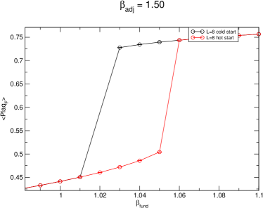
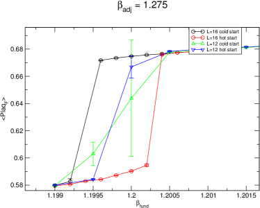
Figure 1: Hysteresis cycle of the fundamental plaquette for different values of the adjoint coupling $\beta_{\rm adj}$. At large $\beta_{\rm adj}$ (left), the separation between the hysteresis branches is visible on relatively small volumes. At smaller $\beta_{\rm adj}$ (right) bigger volumes are necessary to clearly distinguish the first order nature of the transition.

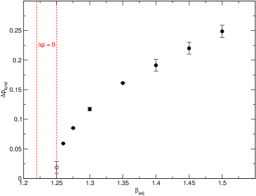
Figure 2: Fundamental plaquette difference between hot and cold start runs at the centre of the hysteresis cycle. Also shown is the approximate position of the critical $\beta_{\rm adj}$ value at which this difference is expected to vanish. A consistent result is found using the adjoint plaquette.

By further decreasing $\beta_{\rm adj}$, the separation between the lower and the upper branch of the hysteresis shows a clear trend suggesting that it should vanish at approximately $\beta_{\rm adj}\lesssim 1.25$. An estimate of this separation is given by the difference of the plaquette in the two vacua at the center of the hysteresis loop:

$$\Delta p_{\rm fund}\;=\;\left\langle{\rm Plaq}_{F,1}\right\rangle-\left\langle{\rm Plaq}_{F,2}\right\rangle\ ,$$ (2)

where the subscripts $1$ and $2$ refer to the disctinct vacua, and a similar definition holds for $\Delta p_{\rm adj}$. This $\Delta p_{\rm fund}$ is plotted in Fig. 2, where we always used the smallest volume where the first order nature of the transition was manifest. The point at $\beta_{\rm adj}=1.25$ required a very large $40^{4}$ lattice for which we currently do not have very good control over the systematic and statistical uncertainties of the simulation.
In the region below the approximate location of the end–point, we have checked that the transition becomes a crossover, signalled by the lack of scaling with the volume in the fundamental and adjoint plaquette susceptibilities. The height and the location of peak of the susceptibility is consistent across the different volumes. The location of the peak separates a strong coupling region at small $\beta_{\rm fund}$ from a region closer to the weak coupling limit ($\beta_{\rm fund}\rightarrow\infty$).

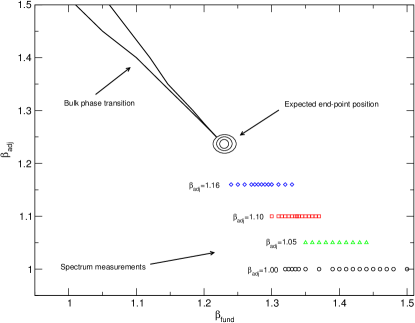
Figure 3: The location of the bulk phase transition is delimited by black lines, representing the extension of the hysteresis cycle. The approximate location of the bulk transition end–point is shown by the arrow. The coloured symbols show the points where the spectrum is investigated.

3 Spectrum measurements

Let us first recall here that we do not want to precisely pin down the end–point location, but rather to identify its neighbourhood, where the spectrum of the theory should be investigated. Our aim is to compare the scaling properties of the spectrum when the bulk transition end–point is approached in a controlled manner, with the ones of the model with $2$ adjoint fermions. This will help us clarify the still controversial nature of this end–point. In Fig. 3 a summary of our results concerning the bulk phase transition line and its end–point is shown. In addition, we indicate the points where we performed a detailed investigation of the spectrum, as described in the following.
Our simulations with the fundamental–adjoint action are carried over using a modified Metropolis algorithm [6] which helps us cope with the increasing autocorrelation times due to critical slowing down when simulating closer to $\beta_{\rm adj}\approx 1.25$. This allows us to obtain a large statistics of independent gauge configurations even on large lattices when the critical slowing down starts affecting the simulations. In particular, we measure our observables on Monte Carlo histories of ${\mathcal{O}}(10000)$ configurations, each separated by ${\mathcal{O}}(100)$ modified–Metropolis updates of the SU(2) link matrices ($\beta_{\rm adj}$ values closer to the end–point have a larger number of intermediate updates between measurements to reduce autocorrelations in our ensembles). In the following, we show results at four different values of the adjoint coupling $\beta_{\rm adj}=1.00,\,1.05,\,1.10,\,1.16$ and spanning a large range of $\beta_{\rm fund}$ such that both regions around the crossover are monitored. A sequence of five different volumes is simulated for each $\beta_{\rm adj}$: $6^{3}\times 12$, $10^{3}\times 20$, $16^{3}\times 20$, $24^{3}\times 32$ and $32^{3}\times 32$, where the longer temporal extent is used to better identify effective mass plateaux.
We employ the variational procedure detailed in Ref. [7] to extract the ground state mass and a few excitations of the spectrum in the following channels:

• String tension: $a\sqrt{\sigma}$ is the lightest dynamical scale in a pure gauge theory and it is used to set the overall scale. We extract the string tension from correlators of long spatial Polyakov loops of length $L=aN_{s}$. The asymptotic large–time behaviour of these correlators is governed by the lightest torelon state whose mass $am_{l}$ can be used to obtain the string tension according to

  $$am_{l}(N_{s})\;=\;a^{2}\sigma N_{s}-\frac{\pi}{3N_{s}}-\frac{\pi^{2}}{18N_{s}^{3}}\frac{1}{a^{2}\sigma}\ .$$ (3)

  The validity of the above equation is checked a posteriori by comparing the extracted string tension with the one obtained using only the leading term $-\pi/(3N_{s})$. Significant finite–size systematics are absent when $L\sqrt{\sigma}>3$, which we satisfied in our simulations using large spatial volumes for the smallest values of $a\sqrt{\sigma}$.

• Scalar glueball mass: $am_{0^{++}}$ is the lightest glueball mass in the spectrum. Correlators of smeared spatial Wilson loops in the scalar representation of the cubic symmetry group are measured on each configuration.

• Tensor glueball mass: $am_{2^{++}}$ is the second lightest glueball and its mass is monitored to check whether its behaviour is the same as the scalar one. Having quantum numbers different from the vacuum, its scaling properties could be different in principle.

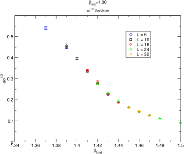
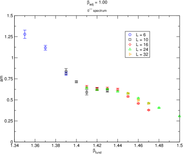
Figure 4: Measured spectrum on different volumes at $\beta_{\rm adj}=1.00$. (left) The square root of the string tension in units of the lattice spacing as $\beta_{\rm fund}$ increases towards the weak coupling region. (right) The mass of the lightest scalar glueball in units of the lattice spacing. Very good control over finite–size effects is obtained for both these observables.

In Fig. 4 we show the string tension and scalar mass at $\beta_{\rm adj}=1.00$ and for a range of different $\beta_{\rm fund}$ and spatial volumes $L^{3}$. The string tension decreases monotonically when approaching the weak–coupling limit at large $\beta_{\rm fund}$, whereas the scalar glueball mass develops a short plateaux in the crossover region before decreasing again. In both cases we have a good control over finite–size effects, with masses matching on at least two subsequent volumes for each point. The largest finite–size effects are seen towards the weak coupling, where the string tension becomes small. Not shown in the plots is the behaviour of the tensor glueball which resembles the string tension one, though with somewhat larger finite–volume systematics.

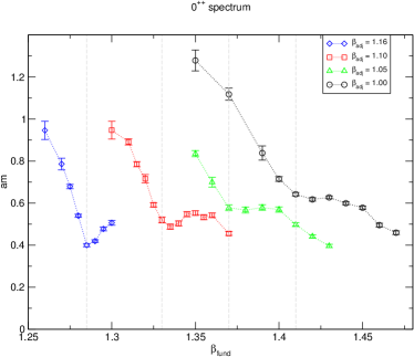
Figure 5: (left) The infinite volume limit of $a\sqrt{\sigma}$ is plotted for $\beta_{\rm adj}$ closer and closer to the end–point location. (right) The scalar glueball mass in the infinite volume limit for all available $\beta_{\rm adj}$. The very different behaviour of the two observables is clear when $\beta_{\rm adj}$ is increased. Also shown are vertical dashed lines highlighting the location of the crossover region.

Given the large range of lattice volume used, we are able to reliably estimate the infinite volume limit of $a\sqrt{\sigma}$ and $am_{0^{++}}$ for all the $\beta_{\rm adj}$ values studied. However, for some of these values we can not extrapolate $am_{2^{++}}$ at $L=\infty$ with our current data. The comparison of the extracted infinite–volume spectrum between different $\beta_{\rm adj}$ is shown in Fig. 5. To study the scaling of the observables along a trajectory when approaching the bulk transition end–point, we choose to follow the line in the phase diagram given by the peak of the fundamental plaquette susceptibility. The location of such peak at the four $\beta_{\rm adj}$ values investigated is highlighted by vertical dashed lines in Fig. 5. On those points, we note that the string tension remains constant when approaching the end–point (larger $\beta_{\rm adj}$), whereas the scalar glueball mass slightly decreases: this suggest a non–constant ratio $m_{0^{++}}/\sqrt{\sigma}$. A summary of this result is shown in Fig. 6.

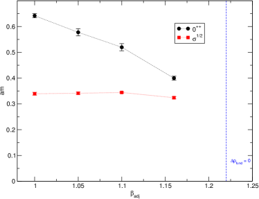
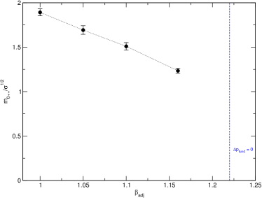
Figure 6: (left) The scalar glueball mass and the square root of the string tension at the values ($\beta_{\rm fund}$,$\beta_{\rm adj}$) defining the plaquette susceptibility’s peak when approaching the end–point from below. (right) The ratio $\frac{m_{0^{++}}}{\sqrt{\sigma}}$ on the same points. We highlighted the approximate location of the bulk transition end–point.

4 Conclusions

In this work we have studied a SU(2) pure gauge theory with a modified lattice plaquette action. We added a coupling to plaquettes in the adjoint representation of the gauge group. This lattice system is known to have a bulk phase transition with an end–point relatively close to the fundamental coupling axis. The nature of this end–point is still controversial and we focused more on the region close to it, but far from the bulk phase transition. Thanks to our improved gluonic spectroscopic technique [7], we measured the string tension, the scalar glueball mass and the tensor one, aiming at studying their scaling properties when the end–point is approached. This is the first study of the gluonic spectrum in this model. Therefore we carefully checked for finite–size systematics and tried to reduce autocorrelation effects on our observables. The extrapolated infinite–volume spectrum shows a non–constant $m_{0^{++}}/\sqrt{\sigma}$ ratio when approaching the end–point in a controlled manner. This seems in contrast with the infrared dynamics of the SU(2) theory with 2 adjoint fermions, where such a ratio is driven by a conformal fixed point and is consistent with the continuum SU(2) Yang–Mills value $m_{0^{++}}/\sqrt{\sigma}\sim 3.7$. The results presented here should be considered as preliminary and might be still too far from the basin of attraction of the end–point. More detailed analysis and discussions will be presented in a forthcoming publication [5].

References

- [1] K. G. Wilson, Confinement of quarks, Phys.Rev., D10 2445, (1974).
- [2] G. Bhanot, M. Creutz, Variant Actions and Phase Structure in Lattice Gauge Theory, Phys.Rev., D24 3212, (1981).
-
[3]
R. V. Gavai, A Study of the bulk phase transitions of the SU(2)
lattice gauge theory with mixed action, Nucl.Phys., B474 446-460, (1996);
S. Datta, R. V. Gavai, Stability of the bulk phase diagram of the SU(2) lattice gauge theory with fundamental adjoint action, Phys.Lett., B392 172-176, (1997). - [4] L. Del Debbio, B. Lucini, A. Patella, C. Pica, A. Rago, Conformal versus confining scenario in SU(2) with adjoint fermions, Phys.Rev., D80 074507, (2009).
- [5] G. Lacagnina, B. Lucini, A. Patella, A. Rago, E. Rinaldi, in preparation.
- [6] A. Bazavov, B. A. Berg, U. M. Heller, Biased metropolis-heat-bath algorithm for fundamental-adjoint SU(2) lattice gauge theory, Phys.Rev., D72 117501, (2005).
- [7] B. Lucini, A. Rago, E. Rinaldi, Glueball masses in the large N limit, JHEP, 08 119, (2010).