Emission lines between 1 and 2 keV in Cometary X-ray Spectra

Abstract

We present the detection of new cometary X-ray emission lines in the 1.0 to 2.0 keV range using a sample of comets observed with the Chandra X-ray observatory and acis spectrometer. We have selected 5 comets from the Chandra sample with good signal-to-noise spectra. The surveyed comets are: C/1999 S4 (linear), C/1999 T1 (McNaught–Hartley), 153P/2002 (Ikeya–Zhang), 2P/2003 (Encke), and C/2008 8P (Tuttle). We modeled the spectra with an extended version of our solar wind charge exchange (SWCX) emission model (Bodewits et al. 2007). Above 1 keV, we find Ikeya–Zhang to have strong emission lines at 1340 and 1850 eV that we identify as being created by solar wind charge exchange lines of Mg XI and Si XIII, respectively, and weaker emission lines at 1470, 1600, and 1950 eV formed by SWCX of Mg XII, Mg XI, and Si XIV, respectively. The Mg XI and XII and Si XIII and XIV lines are detected at a significant level for the other comets in our sample (LS4, MH, Encke, 8P), and these lines promise additional diagnostics to be included in SWCX models. The silicon lines in the 1700 to 2000 eV range are detected for all comets, but with the rising background and decreasing cometary emission, we caution these detections need further confirmation with higher resolution instruments.

1 Introduction

When highly charged ions from the solar wind collide on a neutral gas, the ions get partially neutralized by capturing electrons into an excited state. The subsequent line emission, called solar wind charge exchange emission (SWCX) in X–ray and the Far–UV has been observed in comets, planets, and the ISM. Please see Lisse et al. (1996); Krasnopolsky (1997); Snowden et al. (2004); Bhardwaj et al. (2007); Dennerl (2010) for reviews.

The SWCX process has gained considerable interest recently, as it may contribute a significant amount to the soft X-ray background (Snowden et al. 2004), the interaction of the solar wind and the Earth’s magnetosphere, (Fujimoto et al. 2007; Wargelin et al. 2004) and may be detectable from the exospheres of other stars (Wargelin and Drake 2001). More recently SWCX has also been invoked to explain excess emission in the 2 $-$ 3 keV region from hot diffuse plasma found in galaxies (Liu et al. 2011), star forming regions (Townsley et al. 2011), and from the Cygnus loop supernova remnant (Katsuda et al. 2011), for example.

Cometary SWCX models have evolved over the last several years, from the initial models of Häberli et al. (1997) and Cravens et al. (1997) for example, to models considering the importance of the solar wind properties in emission (Schwadron and Cravens 2000; Kharchenko and Dalgarno 2000, 2001; Beiersdorfer et al. 2003; Kharchenko et al. 2003; Bodewits et al. 2006). The recent survey of a sample of comets observed with Chandra by Bodewits et al. (2007) has shown that the shape of cometary SWCX spectra is predominantly determined by the state of the incoming solar wind. SWCX spectra between 0.3 $-$ 1.0 keV are relatively well understood, aided by a large body of experimental work with hydrogen-like and fully stripped carbon and oxygen ions. This is not the case below 0.3 keV, where there is a forest of emission lines of elements such as Ne, Mg, Si etc. (Schwadron and Cravens 2000) that cannot be distinguished, because of poor instrumental resolution. Observations of comet Schwassmann–Wachmann 3B (73P), a comet that passed within 0.07 AU of Earth, allowing a direct comparison with in situ measurements of the composition of the solar wind, showed that 75 percent of the emission below 300 eV could not be accounted for by carbon ions alone (Wolk et al. 2009).

Similarly, the X-ray spectrum above 1 keV has not been well studied although tentative detections of neon ions, in the 1.1 – 1.2 keV range, were made in the spectrum of the exceptionally X-ray bright comet Ikeya–Zhang presented in Bodewits et al. (2007). Carter et al. (2010) found clear evidence of various Si and Mg, lines in XMM spectra, attributed to interaction of an interplanetary coronal mass ejection with the Earth’s exosphere, and Fujimoto et al. (2007) reported Mg emisson from the north ecliptic pole in Suzaku observations. Quantifying emission lines in this spectral range from comets is the goal of our current work.

Here, we present new line emission features discovered in Chandra cometary X-ray spectra in the 1000 to 2000 eV range. We present details of the Chandra X-ray observations, background subtraction methods, and the SWCX models used in our analysis in Section 2. Results for the X-ray spectra are presented in 3. In Section 4, we discuss our results, line fluxes, line ratios and identifications, and compare these to previous X-ray observations. Lastly, in Section 5 we summarize our findings.

2 Observations and Analysis

2.1 Chandra Observations

Since its launch in 1999, 11 comets have been observed with the Chandra X-ray Observatory and Advanced ccd Imaging Spectrometer (acis). Here, we only include observations made with the acis-S3 chip, which has the most sensitive low energy response. We have selected 5 comets from the Chandra sample with good signal-to-noise spectra and the details of their observations are summarized in Table 1.

ACIS-S is a moderate resolution X-ray imaging CCD with a plate scale of 0.5$\arcsec$/pixel, an instantaneous field of view 8.3$\arcmin\times 8.3\arcmin$, and moderate resolution spectra ($\Delta E\sim$ 110 eV FWHM, $\sigma_{Gaussian}\sim$ 50 eV) in the 300 - 2000 eV energy range. The observations were conducted with the comet’s nucleus near the aim-point in the S3 chip and no active guiding on the comet is used. In this ”drift-scan” method, the comet is centered in the S3 chip and allowed to drift across the chip and the Chandra pointing is updated to re-center the comet before it moves off the chip edge.

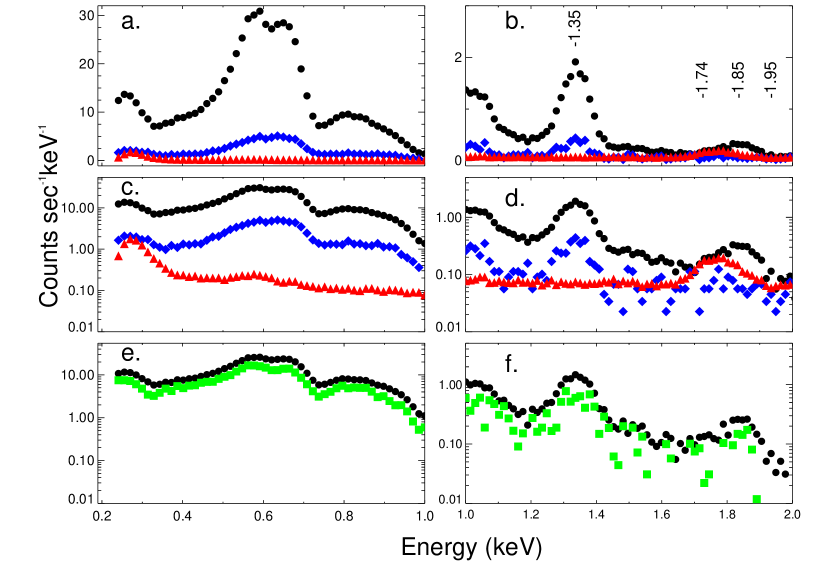
Figure 1: ACIS S3 Spectra of Ikeya–Zhang along with different backgrounds used. Top panels show the ACIS S3 spectra on a linear scale with no background subtracted (filled circles) and over-plotted with the nominal S3 background in blue (diamonds) and the ACIS blank sky background in red (triangles) for: a. the 0.2 – 1.0 keV range and b. the 1.0 – 2.0 keV range (some key energies are noted in panel b). Middle panels, c. and d. are the same as a. and b., but with a log scale for the ordinate. Shown in the bottom panels are IZ spectra with the nominal S3 background spectrum subtracted (filled circles) and over-plotted with the spectrum with 3 times that background subtracted in green (filled squares) for: e. the 0.2 – 1.0 keV range and f. the 1.0 – 2.0 keV range.

Figure 2: ACIS S3 Spectra of Ikeya–Zhang. a. Top panel shows the data (with $\pm 1\sigma$ error bars) and SWCX model fit as a solid histogram. The over-plotted model is our SWCX model including the addition of lines at 1340, 1470, 1600, 1740, 1850, and 1950 eV (see text). b. The middle panel shows the $\chi^{2}$ residuals of the data - model ($\Delta\chi^{2}$) with no additional lines above 1.3 keV, and c. the lower panel, shows the $\chi^{2}$ residuals of the data - model now with the inclusion of lines at 1340 and 1470 eV lines, but no lines at higher energies showing the excess emission between 1600 and 2000 eV.

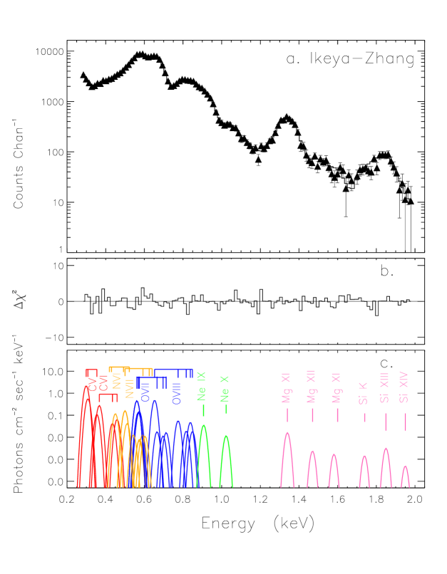
Figure 3: ACIS S3 Spectra of Ikeya–Zhang. a. Shown in the top panel are the data (with $\pm 1\sigma$ error bars) and SWCX model as a solid histogram. b. The middle panel shows the $\chi^{2}$ residuals of the data - model ($\Delta\chi^{2}$). c. The lower panel shows the incident SWCX spectrum and the individual lines ($\sigma\approx$50eV) for CV and CVI (red), NV and NVI (orange), OVII and OVIII (blue) and Ne IX & X (green) and new lines above 1.2 keV as indicated in pink.

Table 1: Sample of Chandra comet observations with observing parameters and solar wind data.

Parameter	LS4	MH	IZ	Encke	8P
Obs. Date	07/14	01/8-15	04/15-16	11/24	1/01-04
	2000	2001	2002	2003	2008
Prop. No.	01100323	02100340	03108076	05100560	09100452
Texp (ks)	9.4	16.9	24	44	47
rh (AU)	0.8	1.26	0.81	0.89	1.10
$\Delta$ (AU)	0.53	1.37	0.45	0.28	0.25
Qgas	3	6-20	20	0.7	2.2
(1028 mols-1)
vp	592	353	372	583	360
(km s${}^{-1})$
Fp	2.9	1.6	3.8	3.2	0.2-0.5
(108 cm-2 s${}^{-1})$

2.2 Analysis

The Chandra data reduction and analysis were done in the same manner as for our previous comet observations (Lisse et al. 2001, 2005; Bodewits et al. 2007; Wolk et al. 2009; Christian et al. 2010) and the reader is referred to these papers for additional details. For each comet, a total image was created from combining each set of observations (obsids). Individual images from these obsids were exposure corrected and remapped into a coordinate system moving with the comet using the sso_freeze algorithm, part of the Chandra Interactive Analysis of Observations (CIAO) software (Fruscione et al. 2006). Spectra and associated calibration products (response matrices and effective areas) were extracted for each comet with the CIAO tools (CIAO v4.3) and analyzed with a combination of IDL and FTOOL packages. Spectral parameters were derived using the least squares fitting technique with the xspec package (Arnaud 1996).

2.2.1 Background Subtraction

Due to the large extent of cometary X-ray emission, and Chandra’s relatively narrow field of view, it is not trivial to obtain a background uncontaminated by the comet and sufficiently close in time and viewing direction. Since our study was motivated by the strong excess emission observed for IZ in the 1300-2000 eV range, it is important to obtain good background subtraction, especially in the 1–2 keV region, where the background counts can be a significant fraction of the cometary source counts.

We tried several different methods for subtracting the background, including using an aperture for the outer region of the S3 chip, regions on the S1 chip, and ACIS observations of other sources at similar galactic latitudes. One problem with subtracting background from the S3 chip is the large physical extent of most comets and having comet photons in these outer regions. Bodewits et al. (2007) used background extracted from the S1 chip, due to several very extended comets, such as Comet Q4 (NEAT). Using the S1 background has the advantage of being at the same time and same particle environment as the S3 observations, but may suffer slightly from poorer low energy response as compared to S3. We also used a 450 ksec ACIS blank sky observation from the Chandra archive. We fit the IZ S3 spectrum with these various backgrounds, still noting important emission lines from the SWCX + higher energy lines ($>$ 1 keV). Shown in Figure 1 are several examples of the IZ spectrum with these different background spectra subtracted. We also summarize several of the important lines in Table 2. The ACIS blank sky observation rises more steeply than our S3 comet background and thus over-subtracts the spectrum above $\approx$1.7 keV. This background also has a strong feature at 1.74 keV, that is probably the result of the local, transient particle background (Markevitch et al. 2003) and we discount this line as real cometary emission. Lines near 1.35 keV are still present for the IZ spectrum when subtracting the ACIS black sky spectrum or even the S3 background raised to 3 times its nominal value. We find that the emission near 1.35 keV is signficant for the IZ spectra with all backgrounds, but the Si emission at 1.74 keV is suspect. We then investigated these 1.8-2.0 keV features using several calibration spectra (such as G 21.5$-$0.9; Tsujimoto et al. (2011), and the Crab; Christian and Swank (1997)) observed with ACIS, and also concluded that these features were not related to calibration issues, such as the Si dead layer, and were true cometary or at least celestial emission.

No comets sampled for this study extended beyond the S3 chip and we therefore used background spectra from the S3 CCD extracted from rectangular areas near its outer edges at distances generally $>8\arcmin$. The subtracted background was then scaled by the ratio of its area relative to the source area. There are likely photons from the comet on the entire S3 chip, and some small iterations in the background scaling factor during fitting were performed as to not over-subtract the background. We feel using the S3 background spectrum at the same time and particle environment provides the most consistent spectral results. In general our results for the 300-1000 eV range are in very good agreement with earlier works (Lisse et al. 2001; Krasnopolsky et al. 2002) and the survey of Bodewits et al. (2007) when our larger extraction area is taken into account.

2.2.2 Spectral Models

We modeled our cometary spectra with a model based on the current SWCX model of Bodewits et al. (2007) extended with individual emission lines to 2000 eV. At first we had modeled the emission in the 280 to 1700 eV range, but then noticed significant emission in the 1700 to 2000 eV range. We then expanded our analysis range up to 2000 eV. In Figure 2 we compare the IZ spectrum fit to 1300 eV to that fit to 2000 eV, showing the need for lines in the 1300 to 1700 eV range and that additional lines in the 1700 to 2000 eV range are also required.

Our model includes the Bodewits et al. 2007 model, originally calculating line strengths from 300 to 1200 eV, now combined with lines above 1200 eV. What follows is a brief description of the Bodewits et al. model which includes lines from C, N, O, and Ne. The Bodewits et al. (2007) SWCX model follows the charge exchange processes between solar wind ions and coma neutrals both in the change of the ionization state of the solar wind ions and in the relaxation cascade of the excited ions. Electron capture by highly charged ions populates highly excited states, which subsequently decay to the ground state. These cascading pathways follow the ionic branching ratios. The absolute intensities of the emission lines are derived from a 3-D integration assuming cylindrical symmetry around the comet–Sun axis. Each group of ions in a species is fixed according to their velocity dependent emission cross sections to the ion with the highest cross section in that group. Thus, the free parameters of our model are the relative strengths of fully stripped- and H–like carbon (CV 299 and C VI 367 eV lines), nitrogen (N VI 419 and NVII 500 eV) and oxygen (O VII 561 and O VII 653 eV) ions, lines for Ne IX at 922 eV and Ne X at 1023 eV and their weaker, but important transitions. This model has 8 groups of fixed lines for C, N, O and Ne plus 6 lines added for the 1200 to 2000 eV range at fixed energies. For our initial fitting, we first allowed the lines to vary within $\pm$30 eV, but found minimal improvement in $\chi^{2}$ and fixed the lines at their laboratory values. All line widths were fixed at the acis-S3 instrument resolution. We note that the charge exchange cross sections for stripped- and H-like Mg and Si are currently lacking in the literature and for this reason we did not link any of the higher energy lines. We used one line at 1340 eV to represent the helium like Mg XI forbidden (f), resonance (r), and intercombination (i) lines, and one line at 1850 eV characterizing helium like Si XIII forbidden (f), resonance (r), and intercombination (i) lines. We also included lines at 1470 (Mg XII Ly $\alpha$), 1600 (Mg XI) , 1740 (Si K), and 1950 eV (Si XIV Ly $\alpha$).

Thus, the spectra were fit in the 280 to 2000 eV range. This provided 118 spectral bins, and 104 degrees of freedom. acis spectra below $\approx$280 eV are discarded because of the rising background contributions, calibration problems and a decreased effective area near the instrument’s carbon edge (the ACIS energy map is only calculated down to 240 eV).

Table 2: IZ Fitted with the SWCX model and different backgrounds

$E_{line}$		Line Flux
(eV)	Line ID	No BG	S3 Bg	S1 BG	Blank Sky	S3 3xBG
299	CV f+r+i	4290$\pm$200	3250$\pm$260	3640$\pm$290	2520$\pm$150	1190$\pm$320
561.1	OVII f+r+i	790$\pm$10	680$\pm$12	630$\pm$12	780$\pm$10	450$\pm$30
1340	Mg XI f+r+i	30$\pm$4	24$\pm$3	23$\pm$5	26$\pm$4	13$\pm$3
1740	Si K	3.1$\pm$0.3	2.0$\pm$0.5	0.8$\pm$0.6	$<$1	$<$2.0
1850	Si XIII f+r+i	7$\pm$0.5	6$\pm$0.6	4$\pm$0.6	0.6$\pm$0.1	2.2$\pm$1
$\chi^{2}$/dof		2.2	1.2	1.8	5.7	0.9
Flux $(0.3-2.0)$ keV		42.6	35.8	32.8	40.7	22.5

3 Results

Our study was motivated by the strong excess emission observed for Ikeya–Zhang in the 1300-2000 eV range, and we confirm significant comet emission in this energy range for comet IZ and several additional comets. The Bodewits SWCX (Solar Wind Charge Exchange) model created for the 300 to 1200 eV range, extended to higher energies produces a $\chi^{2}$ for IZ when fitting the 280 to 2000 eV range of $>$5000 (reduced $\chi^{2}$ $>$ 50). The addition of an emission line at 1340 eV reduces $\chi^{2}$ by 1362. Additional lines at 1470 and 1850 eV lower $\chi^{2}$ by about 200 each. A line at 1740 eV reduced $\chi^{2}$ by 58 but we attribute this to a background feature (discussed below). The addition of a line at 1950 eV marginally reduced $\chi^{2}$ by only 7. Thus, the spectral fit with our SWCX model produced a $\chi^{2}$/dof of 1.2 for IZ and this spectrum, residuals, and model are shown in Figure 3. The addition of the 1340 eV feature to the spectra of the other comets (LS4, MH, 8P and Encke) reduced $\chi^{2}$ by 50 to 200 and the reduced $\chi^{2}$ for our SWCX model range from 0.8 for 8P to 0.9 for MH and 1.23 for LS4. Our SWCX model line fluxes and fit parameters are given in Table 3 and the reductions in $\chi^{2}$ for this model are given in Table 4. The spectral fits for our SWCX model are also shown in Figure 4 for LS4, MH, Encke, and 8P.

Figure 4: Observed spectra for our sample of comets fitted with the SWCX + higher energy line model. The lower panel shown for each spectrum is the $\chi^{2}$ residuals of the data - model ($\Delta\chi^{2}$). The comets shown are: a. C/1999 S4 (linear, LS4), b. C/1999 T1 (McNaught–Hartley, MH), c. 2P/2003 (Encke), and d. C/2008 8P (Tuttle, 8P). (153P/2002 (Ikeya–Zhang), is shown in Figure 3.)

Table 3: SWCX Model Line Flux Results

$E_{line}$		Line Flux
(eV)	Line ID	IZ	LS4	MH	Encke	8P
299	CV f+r+i	3250$\pm$260	330$\pm$50	340$\pm$50	220$\pm$60	430$\pm$90
367.5	CVI Lyα	414$\pm$70	66$\pm$20	54$\pm$14	17$\pm$11	25$\pm$12
419.8	NVI f+r+i	200$\pm$28	38$\pm$13	23$\pm$5	11$\pm$6	13$\pm$7
500.3	NVII Lyα	240$\pm$14	15$\pm$6	21$\pm$2	3$\pm$2	6$\pm$3
561.1	OVII f+r+i	680$\pm$12	73$\pm$4	56$\pm$1	12$\pm$2	20$\pm$2
653.5	OVIII Lyα	714$\pm$10	34$\pm$3	37$\pm$1	2$\pm$1	6$\pm$1
907	Ne IX f+r+i	53$\pm$2	5.5$\pm$0.7	4$\pm$0.5	1.0$\pm$0.2	1.3$\pm$0.2
1024	Ne X	17$\pm$1	6$\pm$1	2.3$\pm$0.5	1.0$\pm$0.3	2.0$\pm$0.3
1340	Mg XI f+r+i	24$\pm$3	6.1$\pm$0.8	2.0$\pm$0.4	1.0$\pm$0.2	1.0$\pm$0.2
1470	Mg XII Lyα	3.5$\pm$0.5	5.7$\pm$0.9	1.7$\pm$0.3	1.0$\pm$0.2	1.4 $\pm$0.2
1600	Mg XI	2.1$\pm$0.6	7.2$\pm$0.4	1.5$\pm$0.5	1.0$\pm$0.2	1.0$\pm$0.3
1740	Si K	2.0$\pm$0.5	7.3$\pm$0.8	3.0$\pm$0.4	1.5$\pm$0.3	2.5$\pm$0.0.3
1850	Si XIII f+r+i	6.0$\pm$0.6	4.2$\pm$0.4	1.7$\pm$0.5	0.8$\pm$0.3	1.5$\pm$0.3
1950	Si XIV Lyα	0.4$\pm$0.5	7.3$\pm$0.8	2.1$\pm$0.4	1.3$\pm$0.2	1.3$\pm$0.3
$\chi^{2}$/dof		1.18	1.23	0.93	1.04	0.80
Flux $(0.30-1.0)$ keV		34.4	3.23	2.66	0.75	1.07
Flux $(0.30-2.0)$ keV		35.8	4.39	3.04	1.10	1.40

Table 4: $\Delta\chi^{2}$ Results for SWCX + Higher Energy Line Model

Region	Eline	Possible ID	Norm	$\Delta\chi^{2}$	$\frac{\chi^{2}}{dof}$
	(eV)		10-5ph cm-2 sec-2
153P/2002
(IZ)	1340	Mg XI f+r+i	24$\pm$3	1362	15.20
	1470	Mg XII Lyα	3.5$\pm$0.5	174	2.95
	1600	Mg XI	2.1$\pm$0.6	67	1.9
	1740	Si K	2.0$\pm$0.5	58	1.76
	1850	Si XIII f+r+i	6.0$\pm$0.6	199	3.21
	1950	Si XIV Lyα	0.4$\pm$0.5	7	1.23
C/1999 S4
(LS4)	1340	Mg XI f+r+i	6.1$\pm$0.8	177	3.07
	1470	Mg XII Lyα	5.7$\pm$0.9	188	3.18
	1600	Mg XI	7.2$\pm$0.4	180	3.1
	1740	Si K	7.3$\pm$0.8	198	3.28
	1850	Si XIII f+r+i	4.2$\pm$0.4	70	1.96
	1950	Si XIV Lyα	7.3$\pm$0.8	181	3.11
C/1999 T1
(MH)	1340	Mg XI f+r+i	2.0$\pm$0.4	50	1.43
	1470	Mg XII Lyα	1.7$\pm$0.3	59	1.52
	1600	Mg XI	1.5$\pm$0.5	48	1.4
	1740	Si K	3.0$\pm$0.4	143	2.36
	1850	Si XIII f+r+i	1.7$\pm$0.5	42	1.34
	1950	Si XIV	2.1$\pm$0.4	94	1.87
2P/2003
(Encke)	1340	Mg XI f+i+r	1.0$\pm$0.2	83	1.86
	1470	Mg XII Lyα	1.0$\pm$0.2	78	1.81
	1600	Mg XI	1.0$\pm$0.2	117	2.3
	1740	Si K	1.5$\pm$0.3	107	2.12
	1850	Si XIII f+r+i	0.8$\pm$0.3	20	1.20
	1950	Si XIV Lyα	1.3$\pm$0.2	116	2.21
8P/Tuttle
(8P)	1340	Mg XI f+r+i	1.0$\pm$0.2	56	1.37
	1470	Mg XII Lyα	1.4$\pm$0.2	141	2.24
	1600	Mg XI	1.0$\pm$0.3	78	1.6
	1740	Si K	2.5$\pm$0.3	295	3.82
	1850	Si XIII f+r+i	1.5$\pm$0.3	69	1.51
	1950	Si XIV Lyα	1.3$\pm$0.3	78	1.60

4 Discussion

Our line fluxes are in good agreement with previous studies of this Chandra sample of comets. Our line fluxes are consistent with Bodewits et al. (2007) when our larger extracted area is taken into account. We extracted spectra from the entire chip, generally about a 1.5 to 2 times larger area than the 7.5$\arcmin$ circular aperture used in Bodewits et al. (2007). We computed X-ray luminosities in the 0.3 to 2.0 keV range from the fluxes for our SWCX model given in Table 2 and Chandra-Earth distances given in Table 1. We find luminosities ranging from 2.0$\times$ 10¹⁴ erg s^-1 for 8P and Encke to 1.7$\times$ 10¹⁵ erg s^-1 for McNaught-Hartley and 2.3 and 2.5 $\times$ 10¹⁶ erg s^-1 for LS4 and IZ, respectively. These values are consistent with previous values in the literature given for the 0.3 to 1.0 keV range for LS4 (Lisse et al. 2001), Encke (Lisse et al. 2005), and 8P (Christian et al. 2010). The luminosities are also consistent with those predicted by SWCX models (Dennerl 2010). The additional 1.0–2.0 keV flux contributes only 4% of the total flux for IZ, 13% of the total flux for McNaught-Hartley, but $\approx$20% of the total flux for 8P and Encke, and nearly 30% of the total flux for Linear S4.

We identify the newly detected feature at 1340 eV as Mg XI (Carter et al. 2010, 2011; Fujimoto et al. 2007). The ACIS S3 does not have the resolution to distinguish between the Mg XI 1330 eV intercombination, the 1344 eV resonance, and 1351 eV forbidden lines, and we fit the spectra with a single line at 1340 eV. This line was significant for all comets in the sample with $\Delta\chi^{2}$ ranging from 50 for MH to over 1300 for IZ. We also detect the Mg XII 1470 eV line at a significant level and the 1600 eV line of Mg XII is marginally detected. Carter et al. (2010) report Mg XI lines at 1.34, 1.6 keV for the Earth’s exosphere and Mg XII at 1.47 keV. Additionally, for comets, Mg was reported in the low energy spectrum of Comet McNaught–Hartley in Krasnopolsky et al. (2002) near 250 eV, near the low energy cut-off of the ACIS-S3 CCD, and Mg ions have solar winds abundances similar to carbon and oxygen. However, searching for low energy emission was beyond the scope of the current work. We have detected a strong feature at 1740 keV for all comets. Djurić et al. (2005) identify the 1740 eV line with charge exchange from neutral silicon K to L and K to M transitions (Si $K-L_{2,3}$,$K-M_{2,3}$), but Carter et al. (2010) identify a feature at 1730 eV as Al XIII. Ranalli et al. (2008) also find a similar feature (near 1740 eV, 7.13 Å) in the XMM spectrum of starburst galaxy M82 and also conclude it is charge exchange from neutral silicon. However, neutral silicon would have to penetrate to the cometary surface in order for this line to possibly undergo charge exchange, and this line is one of the stronger features in the ACIS blank-sky observation (Figure 1). We therefore consider it to be a background feature and not cometary charge exchange emission. Additional features found at 1850 and 1950 eV are identified as Si XIII and Si XIV, respectively (Carter et al. 2010). The 1s2s¹S₀–1s2p³P₁ intercombination interval was measured for helium like silicon by Redshaw and Myers (2002) producing 1850 eV X-rays, suggesting this may contribute to the charge exchange model as well. Once again due to the limitations of ACIS resolution, we must consider the Si XIII line at 1850 eV to contain forbidden line at 1838 eV the 1854 eV intercombination line, and the resonance line at 1863 eV. The Si XIV line at 1950 eV is only marginally detected for IZ, but is significant for the other comets.

Calculating flux ratios of observed emission lines or grouping of these lines is useful for determining relative ionic abundances and hence the solar wind state and conditions in the comet’s nucleus for the optically thin case. These ratios may then be used to test predictions of SWCX models and in separating cometary X-ray spectra into classes (Bodewits et al. 2007). In general carbon and oxygen are the most abundant heavy ions in the solar wind and have produced some of the strongest features reported from cometary X-ray spectra (Cravens et al. 1997; Schwadron and Cravens 2000; Kharchenko and Dalgarno 2000; Krasnopolsky 2006). Thus, the ratio of the sum of the lower energy lines ($\approx$ 300–500 eV) to the strongest feature, OVII is a very sensitive diagnostic to the solar wind conditions (See Figure 6 in Bodewits et al. (2007)). In Figure 5ab we show several line flux ratios as a function of both the OVIII/OVII flux ratio and solar wind velocity. Similar to Bodewits et al. (2007) we find the Carbon + Nitrogen to OVII line ratio (C+N/OVII) to be anti-correlated with the OVIII/OVII ratio. For cold and fast solar wind most of the oxygen is in O⁶⁺ and thus does not contribute to SWCX emission in the X-ray portion of the spectrum and the C+N/OVII ratio is larger. Mg and Si can have significant abundances in the typical solar wind (von Steiger et al. 2000; Zurbuchen et al. 2002). Our higher energy lines of Mg XI and Si line ratios also show a similar trend to the C+N/OVII ratios, decreasing with an increase in the OVIII/OVII ratio. We find MgXI/OVII ratios ranging from 0.04 for IZ to 0.17 for LS4. These are similar to the MgXI/OVII ratio of 0.04 found for the SWCX contribution of the X-ray background (Snowden et al. 2004) and 0.14 found by Fujimoto et al. (2007) for the Earth’s magnetosheath, but much lower than the ratio of 0.28 that Carter et al. (2010) found for the Earth’s exosphere after a coronal mass ejection (CME) event. Our measured Si XIII/OVII ratios range from 0.01 for IZ to 0.08 for 8P and similar to the Mg ratios, but they are smaller than the ratio of 0.30 found by Carter et al. (2010).

CMEs and interplanetary CME’s (ICME’s) can cause unusually high charge states of C, O, Ne, Si, Mg, and Fe in the solar wind (Snowden et al. 2004; Gruesbeck et al. 2011). Gruesbeck et al. (2011) show that silicon primarily has charge states of Si⁸⁺ to Si⁹⁺ for a typical solar wind and this is shifted to Si¹⁰⁺ and Si¹¹⁺ for ICME plasma solar wind and their time-of-flight instruments are limited to charge states between 8+ and 12+. Our Chandra results confirm moderate to strong Si emission for all comets in our sample from charge states of Si¹³⁺ to Si¹⁴⁺, but with the limited resolution and exposure times of most Chandra observations, a deep observation of a very active and X-ray bright comet is needed to search for additional charge states of Si.

No strong trends are seen for these line ratios as a function of solar wind velocity, but as discussed in Bodewits et al. (2007) the velocity alone does not give a good indication of the solar wind state and underlying ioinic composition. Additionally, above $\approx$300 km s^-1, the charge exchange cross sections change only slightly with SW velocity (Schwadron and Cravens 2000; Lisse et al. 2005). However, the similar trends for Mg and Si ratios observed for the C+N ratios promise these features can be used for future diagnostics.

Figure 5: Flux ratios for our sample comets. Shown in the left panel are flux ratios as a function of the OVIII/OVII ratio for the sum of the strongest carbon + nitrogen lines (C+N, top), Mg lines (middle) and Si (bottom panel). The right panel shows the same ratios as a function of solar wind velocity (see text).

5 Conclusions

We have detected new line emission in the 1300-2000 eV range for several comets observed with Chandra ACIS spectrometer. The typical, previously reported emission lines in the 300 to 1000 eV range are detected for all comets from CV, CVI, NVI, NVII, OVII, OVIII, Ne IX, Ne X, and line strengths correlate with the charge state of the solar wind continuing credence for the idea that these lines are formed by solar wind charge exchange. Above 1 keV, we find Ikeya–Zhang to have strong emission lines at 1340 and 1850 eV that we identify as being created by solar wind charge exchange lines of Mg XI and Si XIII, respectively, and weaker emission lines at 1470, 1600, and 1950 eV formed by SWCX of Mg XII, Mg XI, and Si XIV, respectively. The Mg XI 1340 line is significant for the other comets in our sample (LS4, MH, Encke, 8P). Additional Mg lines in the 1400 to 1600 eV range are detected for all comets in our sample at a significant level and promise additional diagnostic lines to be added to SWCX models. The Si XIII line at 1850 eV is detected for all comets in our sample. The Si XIV is only marginally detected for IZ, but is signifcant for the other comets in our sample. Although the silicon lines in the 1700 to 2000 eV range are detected for all comets, with the rising background and decreasing cometary emission, we caution these detections need further confirmation with higher resolution instruments.

References

- Arnaud (1996) Arnaud, K. 1996, Astronomical Data Analysis Software and Systems V (ASP Conf. Ser. 101), ed. G. H. Jacoby & J. Barnes (San Francisco, CA: ASP), 17
- Beiersdorfer et al. (2003) Beiersdorfer, P. et al., 2003, Science, 300, 1558
- Bhardwaj et al. (2007) Bhardwaj, A., et al. 2007, Planet. Space Sci., 55, 1135
- Bodewits et al. (2006) Bodewits, D., Hoekstra, R., Seredyuk, B., R. W. McCullough, G. H. Jones & A. G. G. M. Tielens, 2006, ApJ, 642, 593
- Bodewits et al. (2007) Bodewits, D., Christian, D.J., Torney, M., et al. 2007, A&A, 469, 1183
- Carter et al. (2010) Carter, J. F., Sembay, S., Read, A. M., 2010, MNRAS, 402, 867
- Carter et al. (2011) Carter, J. F., Sembay, S., Read, A. M., 2011, A&A, 527, 115
- Christian and Swank (1997) Christian, D. J., Swank, J. H., 1997, ApJS, 109, 177
- Christian et al. (2010) Christian, D. J., Bodewits, D., Lisse, C. M., et al., 2010, ApJS, 187, 447
- Cravens et al. (1997) Cravens, T., 1997, Geophys. Res. Lett., 24, 105
- Dennerl et al. (1997) Dennerl, K., et al., 1997, Science, 277, 1625
- Dennerl (2010) Dennerl, K., 2010, SSR, 157, 57
- Djurić et al. (2005) Djurić, N., Lozano, J. A., Smith, S. J., Chutjian, A., 2005, ApJ, 635, 718
- Fruscione et al. (2006) Fruscione, A. et al. 2006, Proc. SPIE, 6270, 60
- Fujimoto et al. (2007) Fujimoto, R., et al., 2007, PASJ, 59,133
- Gruesbeck et al. (2011) Gruesbeck, J.R., Lepri, S.T., Zurbuchen, T.H., Antiochos, S.K., 2011, ApJ, 730, 103
- Häberli et al. (1997) Häberli, R. M., Gombosi, T. I., DeZeeuw, D. L., Combi, M. R., Powell, K. G., 1997, Science, 276, 939
- Katsuda et al. (2011) Katsuda, S. et al., 2011, ApJ, 730, 24
- Kharchenko and Dalgarno (2000) Kharchenko, V., Dalgarno, A., 2000, J. Geophys. Res., 105, 18351
- Kharchenko and Dalgarno (2001) Kharchenko, V., Dalgarno, A., J., 2001, ApJ, 554, 99
- Kharchenko et al. (2003) Kharchenko, V., Rigazio, M., Dalgarno, A., Krasnopolsky, V. A., 2003, ApJ, 585, 73
- Krasnopolsky (1997) Krasnopolsky, V. A., 1997, Icarus, 128, 368
- Krasnopolsky et al. (2002) Krasnopolsky, V. A., Christian, D. J., Kharchenko, V., Dalgarno, A., Wolk, S. J., Lisse, C. M., Stern, S. A., 2002, Icarus, 160, 437
- Krasnopolsky (2006) Krasnopolsky, V. A., 2006, J. Geophys. Res., 111, A12102
- Lisse et al. (1996) Lisse, C. M. et al., 1996, Science, 274, 205
- Lisse et al. (2001) Lisse, C. M. et al., 2001, Science, 292, 1343
- Lisse et al. (2005) Lisse, C. M., Christian, D. J., Dennerl, K., et al., 2005, ApJ, 635, 1329
- Liu et al. (2011) Liu, J., Wang Q. D., Mao S., MNRAS, 2011, 415, L64
- Markevitch et al. (2003) Markevitch, M. et al. 2003, ApJ, 583, 70
- Ranalli et al. (2008) Ranalli, P., Comastri, A., Origlia, L., Maiolino, R., 2008, MNRAS, 386, 1464
- Redshaw and Myers (2002) Redshaw, M., Myers, E.G., 2002, Physical Review Letters, 88, 3002
- Schwadron and Cravens (2000) Schwadron, N. A., Cravens, T. E., 2000, ApJ, 544, 558
- Snowden et al. (2004) Snowden, S. L. et al., 2004, ApJ, 610, 1182
- Townsley et al. (2011) Townsley, L. et al., 2011, ApJS, 194, 15
- Tsujimoto et al. (2011) Tsujimoto, M. et al., 2011, A&A, 525, 25
- von Steiger et al. (2000) von Steiger et al. 2000, J. Geophys. Res., 105, 27217
- Wargelin and Drake (2001) Wargelin, B. J., Drake, J. J. 2001, ApJ, 546, 57
- Wargelin et al. (2004) Wargelin, B. J., et al., 2004, ApJ, 607, 596
- Wolk et al. (2009) Wolk, S. J., Lisse, C. M., Bodewits, D., Christian, D. J., Dennerl, K., ApJ, 694, 1293
- Zurbuchen et al. (2002) Zurbuchen, T. H., Fisk, L.A., Gloeckler, G., von Steiger, R. 2002, Geophys. Res. Lett., 29, 66