ELEMENTAL ABUNDANCES AND THEIR IMPLICATIONS FOR THE CHEMICAL ENRICHMENT OF THE BOÖTES I ULTRA-FAINT GALAXY

Abstract

We present a double-blind analysis of high-dispersion spectra of seven red giant members of the Boötes I ultra-faint dwarf spheroidal galaxy, complemented with re-analysis of a similar spectrum of an eighth member star. The stars cover [Fe/H] from –3.7 to –1.9, and include a CEMP-no star with [Fe/H] = –3.33. We conclude from our chemical abundance data that Boötes I has evolved as a self-enriching star-forming system, from essentially primordial initial abundances. This allows us uniquely to investigate the place of CEMP-no stars in a chemically evolving system, in addition to limiting the timescale of star formation. The elemental abundances are formally consistent with a halo-like distribution, with enhanced mean [$\alpha$/Fe] and small scatter about the mean. This is in accord with the high-mass stellar IMF in this low-stellar-density, low-metallicity system being indistinguishable from the present-day solar neighborhood value. There is a non-significant hint of a decline in [$\alpha$/Fe] with [Fe/H]; together with the low scatter, this requires low star formation rates, allowing time for SNe ejecta to be mixed over the large spatial scales of interest. One star has very high [Ti/Fe], but we do not confirm a previously published high value of [Mg/Fe] for another star. We discuss the existence of CEMP-no stars, and the absence of any stars with lower CEMP-no enhancements at higher [Fe/H], a situation which is consistent with knowledge of CEMP-no stars in the Galactic field. We show that this observation requires there be two enrichment paths at very low metallicities: CEMP-no and “carbon-normal”.

1. INTRODUCTION

The Boötes I ultra-faint dwarf spheroidal galaxy was discovered by Belokurov et al. (2006), who reported an absolute magnitude M${}_{V,\,total}=-5.8$ and half-light radius $\sim 220$ pc, noting that its magnitude “makes it one of the faintest galaxies known”. This discovery has been followed by a large number of investigations of the spatial, kinematic, and chemical abundance distributions of Boötes I, all aiming to provide insight into the formation and evolution of this extremely low luminosity galaxy, and into what it has to tell us about conditions at the earliest times. Photometric studies indicate an exclusively old stellar population. We refer the reader to the works of Belokurov et al. (2006), Dall’Ora et al. (2006), Fellhauer et al. (2008), Feltzing et al. (2009), Koposov et al. (2011), Lai et al. (2011), Martin et al. (2007, 2008), Muñoz et al. (2006), Norris et al. (2008, 2010c, 2010b), and Okamoto et al. (2012) for details of progress to date. Two fundamental results have emerged. The first is that this low luminosity galaxy is dark-matter dominated, with a mass-to-light ratio within the half-light radius estimated to lie in the range 120 $<M/L<$ 1700 (Martin et al. 2007; Wolf et al. 2010; Koposov et al. 2011). The kinematics may be complex: Koposov et al. (2011) tentatively identify two kinematically distinguishable components, and speculate that this “reflects the distribution of velocity anisotropy in Boötes I, which is a measure of its formation processes.” The second result is that there is also a large dispersion in chemical abundances within the system, indicative of self-enrichment: for iron the range is $-3.7<$ [Fe/H] $<-1.9$; there is a wide range in the relative abundance of carbon: –0.8 $<$ [C/Fe] $<$ +2.2 (Norris et al., 2010b; Lai et al., 2011); and Feltzing et al. (2009) describe one object with an atypically high value of [Mg/Ca] $\sim$ +0.7.

Boötes I is one of the brighter of some 15 newly recognized ultra-faint dwarf galaxy satellites of the Milky Way, which are the subject of considerable current activity, driven by their potential to provide an understanding of fundamental questions on the formation and evolution of galaxies (see, e.g., Gilmore et al. 2007 and references therein). For example, why are there considerably fewer dwarf galaxy satellites of the Milky Way than predicted by the $\Lambda$CDM paradigm; what is the connection between their bright and dark matter; when and where did their baryonic component form; and what has driven their chemical abundance inhomogeneities?

The present paper is the fourth in a series aimed at understanding the chemical abundance characteristics of Boötes I, and their implications for the chemical enrichment of the system and the manner in which it formed. The first (Norris et al., 2008) reported abundances for 16 radial-velocity members based on medium-resolution spectra (R $\sim 5000$): we found an abundance range of $\Delta$[Fe/H]$\sim 2.0$ dex, with one star (Boo-1137) having [Fe/H] $\sim-3.4$. The second (Norris et al., 2010c) confirmed the extremely metal-poor nature of Boo-1137 based on high-resolution (R $\sim 40,000$), high-$S/N$ ($S/N\sim 20-90$), spectroscopy: this star has [Fe/H] = –3.7, and relative-abundance ratios for some 15 additional elements that are comparable to those of extremely metal-poor stars of similar [Fe/H] in the Galactic halo. In the third paper (Norris et al., 2010b), we determined carbon abundances ([C/Fe]) for the 16 radial-velocity members reported in the first paper, together with preliminary values of [Fe/H] for seven of these stars for which we had obtained high resolution (R $\sim 45000$) spectroscopy: our conclusion was that the abundance dispersion was real, and the distribution of the carbon abundances in these red giants was not unlike that of the Galactic halo.

The purpose of this paper is to report the data of the seven high-resolution spectra noted above, to present abundance measurements for 14 elemental species, and to consider both systematic and random uncertainties in our results. In Section 2 we describe the observational material and the measurement of line strengths and radial velocities, while in Sections 3 and 4 we analyze these to produce and present chemical abundances. As part of our measurement and abundance determination, we adopt a double-blind methodology that employs two distinct analyses of the dataset in order to permit us to obtain an independent assessment of the errors associated with our results. Finally, in Section 5 we discuss the implications of our results for the chemical evolution of Boötes I and chemical enrichment at the earliest times.

1.1. Double-blind Analysis

Detection of a range of abundances in an ultra-faint dSph galaxy, and especially detection of either or both of a real range in elemental abundance ratios at a given iron abundance, or a trend in elemental abundance ratios as a function of iron abundance, provides constraints on the rate of star-formation and associated self-enrichment, and the efficiency, timescale, and length scale of mixing in the interstellar medium at very early times. Hence, understanding both systematic and random measuring errors is an essential aspect of an analysis. Before proceeding to determine abundances from these spectra of stars in Boötes I, and in an effort to obtain an external estimate of the abundance accuracy that independent researchers might achieve from spectra of the quality we have available, the decision was taken to perform two independent analyses. We refer the reader to Bensby et al. (2009) for an earlier example of this type of approach. It was agreed that J.E.N. and D.Y. (working together, and hereafter referred to as NY) would perform one analysis, while D.G. and L.M. (also working together, and referred to as GM) would perform the other. There would be no correspondence or discussion between NY and GM in this first phase of the project. Both groups would use their standard approaches, line lists, etc, consistent with their previous published studies. The reader will see this reflected in Sections 2.2 – 3.4, which describe the measurement and analysis of our spectra to produce radial velocities, stellar atmospheric parameters, and chemical abundances.

2. HIGH-RESOLUTION SPECTROSCOPY

2.1. Observational Data

High-resolution, moderate-$S/N$, spectra were obtained of seven Boötes I red giants as part of a larger program to investigate the kinematics and chemical abundances of the Boötes I system. During 2009 February – March, data were obtained with the FLAMES spectrograph of the 8.2 m Kueyen (VLT/UT2) telescope at Cerro Paranal, Chile. We used FLAMES in UVES-Fiber mode (Pasquini et al., 2002): 130 fibers fed the medium-resolution Giraffe spectrograph, while eight additional fibers led to the high-resolution Ultraviolet-Visual Echelle Spectrograph (UVES). We refer the reader to Koposov et al. (2011) for the kinematic analysis of the medium-resolution data: the UVES spectra are the subject of the present work. Of the eight UVES fibers, seven were allocated to the Boötes I members and one to a nearby sky position to permit background measurement. 22 useful individual exposures were obtained in Service Mode, most of duration 46 min, leading to an effective total integration time of 17.2 hrs. The spectra were obtained using the 580nm setting and cover the wavelength ranges 4800 – 5750 Å and 5840 – 6800 Å, and have resolving power R = 47,000.

Details of the seven program stars are presented in Table 1. Six of them were taken from the sample of Norris et al. (2008), who used medium-resolution spectra to obtain initial estimates of [Fe/H]. The seventh is from Table 1 of Martin et al. (2007), where it is the sixty-third entry. In what follows we shall refer to this object as Boo-119, consistent with the identification system adopted by Norris et al. (2008). In the present Table 1, columns (1) – (2) present the identifications of Norris et al. (2008), and of Martin et al. (2007) or Lai et al. (2011), respectively, while columns (3) – (4) contain coordinates. Column (5) – (6) present SDSS Data Release 7 (Abazajian et al. 2009) $ugriz$ photometry $g_{0}$ and $(g-r)_{0}$ (where a reddening of E($B-V$) = 0.02 (Belokurov et al., 2006) has been adopted). Finally, columns (7) – (9) contain [Fe/H] values determined from medium-resolution spectroscopy by Norris et al. (2008, R $\sim 5000$), Martin et al. (2007, R $\sim 8500$), and Lai et al. (2011, R $\sim 1800$) using the Ca II K line, the Ca II infrared triplet, and the blue spectral region, respectively. All stars have projected distances from the nominal centre of Boötes I that are well within one half-light radius and have radial velocities and values of [Fe/H] consistent with membership of Boötes I (see Sections 2.2 and  3 below).

Table 1THE SEVEN BOÖTES I RED-GIANT PROGRAM STARS

Star	Other	RA	Dec	$g_{0}$	$(g-r)_{0}$	[Fe/H]	[Fe/H]	[Fe/H]
	ID	(2000)	(2000)
(1)	(2)	(3)	(4)	(5)	(6)	(7)	(8)	(9)
33	… …	14 00 11.73	+14 25 01.4	18.155	0.736	–2.96	…	…
41	66 29	14 00 25.83	+14 26 07.6	18.304	0.697	–2.03	–1.6	–1.65
94	… …	14 00 31.51	+14 34 03.6	17.449	0.872	–2.79	…	…
117	4 1	14 00 10.49	+14 31 45.5	18.134	0.746	–1.72	–2.2	–2.34
119	63 21	14 00 09.85	+14 28 22.9	18.359	0.728	…	–2.7	–3.79
127	… …	14 00 14.57	+14 35 52.7	18.087	0.773	–1.49	…	…
130	… …	13 59 48.98	+14 30 06.2	18.136	0.707	–2.55	…	…

The spectra of each individual exposure of the seven Boötes I stars were reduced with the FLAMES-UVES pipeline. Examples of reduced, co-added, and continuum-normalized spectra of the seven program stars, in the region of the Mg I b lines (at 5169.3, 5172.7, and 5183.6 Å), are shown in Figure 1, together with that of Boo-1137 from the work of Norris et al. (2010c). Effective temperatures and surface gravities derived in the analysis below are also included in the figure. A large range in line strength among the sample is clearly evident and as will be demonstrated in the analysis that follows, a large range in chemical abundance, of order $\Delta{\rm[X/H]}=1.8$ dex, is required to explain these differences.

Figure 1.— Spectra of the Boötes I giants (including Boo-1137 from Norris et al. 2010c) in the region of the Mg b lines. Mean adopted values of $T_{\rm eff}$/$\log g$ are also presented.

2.2. Radial Velocities

Radial velocities were determined independently by NY and GM for the individual spectra described in Section 2.1, in order to confirm membership of Boötes I and to complement the medium-resolution Giraffe-based investigation of Koposov et al. (2011).

2.2.1 NY analysis

Following Norris et al. (2010c, Section 2.4), radial velocities were measured over the wavelength range 5160 – 5190 Å, which contains the relatively strong Mg I b lines, for each of the individual exposures. This was achieved by Fourier cross-correlation (using ‘scross’ in the FIGARO reduction package) against a synthetic spectrum having $T_{\rm eff}$ = 4700 K, $\log g$ = 1.5, [M/H] = –2.5, and microturbulent velocity $\xi_{t}$ = 2 km s^-1 (computed with the code described by Cottrell & Norris (1978), model atmospheres of Kurucz (1993a), and atomic line data from VALD). The resulting heliocentric radial velocities are presented in Table 2, where columns (1) – (4) contain the star name, radial velocity, (internal) standard error, and the number of individual spectra that were measured, respectively. The internal accuracy is 0.3 km s^-1, small compared with the full velocity spread of 15 km s^-1.

Table 2RADIAL VELOCITIES FOR PROGRAM STARS

Star	Vr(NY)	s.e.Vr(NY)	No.	Vr(GM)	s.e.Vr(GM)	No.	Vr
	(km s-1)	(km s-1)		(km s-1)	(km s-1)		(km s-1)
(1)	(2)	(3)	(4)	(5)	(6)	(7)	(8)
33	102.11	0.31	21	102.18	0.08	22	102.15
41	106.91	0.29	21	106.97	0.10	22	106.94
94	95.34	0.28	21	95.51	0.14	22	95.43
117	99.45	0.30	21	99.64	0.08	22	99.54
119	91.75	0.30	20	93.25	0.33	22	92.50
127	100.28	0.31	21	100.24	0.09	22	100.26
130	104.85	0.27	21	104.60	0.10	22	104.72

2.2.2 GM analysis

Radial velocities were determined by using the IRAF tasks ‘fxcor’ and ‘rvcorrect’ to cross-correlate the individual observed spectra over the wavelength range 4900 – 5700 Å against the synthetic, high-resolution, spectrum of the Coelho et al. (2005) model atmosphere having $T_{\rm eff}$ = 4500 K, $\log g$ = 1.5, [Fe/H] = –2.0, and [$\alpha$/Fe] = +0.4. The resulting heliocentric velocities, internal errors, and number of spectra analyzed are shown in columns (5) – (7) of Table 2. The mean internal precision of the velocities is $\sim 0.13$ km s^-1, while the full velocity spread is 14 km s^-1.

2.2.3 Adopted Velocities

The agreement between the NY and GM velocities is excellent, with the mean difference between the two determinations being –0.2 km s^-1 with dispersion 0.6 km s^-1. If one were to exclude Boo-119 (the most metal-poor star, where template mismatch is anticipated to have degraded the measurement accuracy) these numbers become –0.1 km s^-1 and 0.1 km s^-1, respectively. The average values of the NY and GM velocities for individual stars are given in column (8) of Table 2. These lead to the mean value for the sample of 100.2 $\pm$ 1.9, with dispersion 5.0 $\pm$ 1.3. The individual velocities in column (8) confirm that all of the seven stars have values consistent with their being members of Boötes I.

2.2.4 Comparison with the results of Koposov et al. (2011)

The present UVES-based mean velocity and dispersion are consistent with the Giraffe-based values of Koposov et al. (2011), who obtained 101.8 $\pm$ 0.7 km s^-1 and 4.6 ${}^{+0.8}_{-0.6}$ km s^-1, respectively, in their analysis of a sample of some 100 Boötes I members. Koposov et al. (2011) reported that their derived stellar radial velocities could be equally well-fit by models having a single component with dispersion 4.6 ${}^{+0.8}_{-0.6}$ km s^-1, or two kinematically distinct components – the first with velocity dispersion 2.4 ${}^{+0.9}_{-0.5}$ km s^-1 which comprises 70% of the system, and the second with dispersion “around” 9 km s^-1 making up the remaining 30%. Bearing in mind that our UVES data and the Giraffe results probe the same projected distances from the centre of Boötes I, we tested whether our radial velocity data are consistent with this two-component model using Monte Carlo analysis as follows. Assuming Gaussian velocity distributions for the two components of Koposov et al. (2011), we drew 10000 samples of seven stars at random and computed their velocity dispersion. We found that values greater than or equal to the observed dispersion of 5 km s^-1 are expected relatively frequently, some $\sim 28\%$ of the time.

2.3. Stellar Atmospheric Parameter Determination

2.3.1 NY analysis

In order to perform model atmosphere abundance analyses, one needs the atmospheric parameters $T_{\rm eff}$ and $\log g$. For the NY analysis our values are those presented by Norris et al. (2010b, Section 5 and Table 3), which we reproduce here in columns (2) and (3) of Table 3. While we refer the reader to the earlier work for details, we note here that (i) temperatures are based on calibrations of $B-V$ and $griz$ photometry following Norris et al. (2008) and Castelli, respectively, and (ii) gravities were obtained by comparing the colors with those of the Yale–Yonsei (YY) Isochrones (Demarque et al., 2004) adopting an age of 12 Gyr, and the assumption that the stars lie on the red giant branch of the system. These determinations require chemical abundance as an input parameter: the medium-resolution [Fe/H] values of Norris et al. (2008) and Martin et al. (2007) (see columns (7) and (8) of our Table 1, respectively) were used to provide first estimates of $T_{\rm eff}$ and $\log g$ and thence model atmosphere abundances, and the process iterated until self-consistent values were obtained.

Table 3ATMOSPHERIC PARAMETERS FOR PROGRAM STARS

Star	$T_{\rm eff}$(K)	$\log g$	[Fe/H]	$\xi_{t}$	$T_{\rm eff}$(K)	$\log g$	[Fe/H]	$\xi_{t}$	$T_{\rm eff}$(K)	$\log g$	[Fe/H]	$\xi_{t}$
	(NY)	(NY)	(NY)	(NY)	(GM)	(GM)	(GM)	(GM)	(F09)	(F09)	(F09)	(F09)
(1)	(2)	(3)	(4)	(5)	(6)	(7)	(8)	(9)	(10)	(11)	(12)	(13)
33	4730	1.4	–2.36	2.8	4750	1.4	–2.28	2.0	4600	1.0	–2.52	2.1
41	4750	1.6	–1.96	2.8	4800	1.4	–1.80	2.1	…	…	…	…
94	4570	0.8	–2.97	3.3	4550	0.9	–2.91	2.0	$<$4600	0.5	–2.95	2.1
117	4700	1.4	–2.31	2.7	4750	1.4	–2.05	1.8	4600	1.0	–2.29	2.1
119	4790	1.4	–3.21	2.4	4750	1.4	–3.44	2.9	…	1.0	…	…
127	4670	1.4	–2.11	2.7	4700	1.4	–1.92	2.0	4600	1.0	–2.03	2.1
130	4750	1.4	–2.35	2.6	4800	1.4	–2.28	2.1	…	1.0	…	…

2.3.2 GM analysis

The stellar atmospheric parameters $T_{\rm eff}$ and $\log g$ were determined by GM by comparing the SDSS $gr$ photometry presented in Table  1 with the BaSTI $\alpha$-enhanced isochrones (Pietrinferni et al., 2006) in the ($M_{g}$, $g-r$) (absolute magnitude, color) – plane for an adopted age of 12 Gyr, a distance modulus of $(m-M)_{0}$ = 19.10 (Dall’Ora et al., 2006), and a reddening of E($B-V$) = 0.02. This process also requires an estimate of metallicity. Based on an iterative abundance procedure, GM adopted isochrones having [Fe/H] = –2.6 for Boo-94 and Boo-119, and –2.1 for the other stars. GM’s adopted values of $T_{\rm eff}$ and $\log g$ are presented in columns (6) and (7) of Table 3.

2.4. Equivalent Widths

2.4.1 NY measurements

The individual ESO VLT pipeline-reduced spectra were first cross-correlated to determine relative wavelength shifts between them in order to compensate for the Earth’s motion during the $\sim 40$ day data-taking interval. After sky-subtracting and shifting the individual spectra to the rest frame, NY co-added and then double-binned them into pixels of width 0.028 Å and 0.034 Å (for the shorter and longer wavelength regions described in Section 2.1). These spectra were smoothed with a Gaussian of standard deviation $\sim 0.025$ Å to produce final spectra for the seven program stars. For six of the stars the $S/N$ per 0.03 Å pixel at 5500 Å was 25 – 35, while for the seventh (Boo-94) it was 60.

Equivalent widths were measured independently by each of J.E.N. and D.Y. for a set of unblended lines taken from the list of Cayrel et al. (2004) (as described by Norris et al. (2010c) in our analysis of the extremely metal-poor red giant Boo-1137) with techniques described by Norris et al. (2001) and Yong et al. (2008). J.E.N. and D.Y. compared their results and excluded from further consideration lines for which their measured equivalent widths differed by more than 15 mÅ. The resulting two sets of line strengths are compared for the seven Boötes I giants in the left panels of Figure 2. While small departures from the one-to-one line are evident in the figure, representing a systematic difference of a few mÅ, NY chose to simply average their two measursements. The resulting line strengths in Table 2.4.1 for 115 unblended lines are suitable for model atmosphere abundance analysis. Line identifications, lower excitation potentials, $\chi$, and log $gf$ values are presented in columns (1) – (4) of the table.

Figure 2.— Comparison of equivalent widths of (left) J.E.N. and D.Y., and (right) NY and GM for the seven Boötes I giants, as described in the text. (For convenience of presentation, individual stars have been offset by multiples of 100 mÅ in the vertical direction.)

Table 4NY ATOMIC DATA, EQUIVALENT WIDTHS (mÅ), AND ABSOLUTE ABUNDANCES

Spec.	$\lambda$	$\chi$	log $gf$	EW	log $\epsilon$	EW	log $\epsilon$	EW	log $\epsilon$	EW	log $\epsilon$	EW	log $\epsilon$
	(Å)	(eV)		Boo33	Boo33	Boo41	Boo41	Boo94	Boo94	Boo117	Boo117	Boo119	Boo119
(1)	(2)	(3)	(4)	(5)	(6)	(7)	(8)	(9)	(10)	(11)	(12)	(13)	(14)
Na I	5895.92	0.00	$-$0.19	191.0	3.90	…	…	164.5	3.22	…	…	155.0	3.73
Mg I	5528.40	4.34	$-$0.34	108.0	5.42	168.5	6.16	81.3	4.98	104.5	5.36	90.7	5.33
Ca I	5349.47	2.71	$-$0.31	17.5	4.00	59.8	4.70	…	…	31.0	4.28	…	…
Ca I	5581.98	2.52	$-$0.71	…	…	46.3	4.69	…	…	37.2	4.55	…	…
Ca I	5588.75	2.52	0.21	82.4	4.27	118.5	4.72	…	…	83.6	4.27	18.0	3.32

References. — Notes.   (This table is available in its entirety in a machine-readable form in the online journal. A portion is shown here for guidance regarding its form and content.)

2.4.2 GM measurements

After sky-subtraction, the individual stellar spectra had radial velocities determined as described above. For each star, the individual spectra were then reduced to the rest-frame, continuum-normalized and median-combined. In order to increase the $S/N$ ratio used for the abundance analysis, the spectra were then double-binned, obtaining a step of 0.028 Å  and 0.034 Å  per pixel in the 4800 – 5750 Å and 5840 – 6800 Å  regions, respectively. The spectra were further smoothed with a Gaussian having standard deviation of 0.035 Å, which caused a negligible loss of resolution, from the nominal initial R = 47000 to R = 45000.

Equivalent widths were determined for a set of lines assembled from a number of literature references (see Monaco et al. 2011), and for which atomic parameters were obtained from the Vienna Atomic Line Database (VALD)(Kupka et al., 2000), except for Fe II, for which GM adopted the log $gf$ values of Meléndez & Barbuy (2009). With one exception, the line strengths were measured by using Gaussian fitting with the ‘fitline’ code developed by P. François (private communication; see Lemasle et al. 2007). All lines were inspected by eye and the continuum re-defined interactively. The code allows for deblending as well. The exception noted above was Na, for which measurement was achieved using IRAF/splot. For the Na lines, which have strengths greater than 150 mÅ, Voigt rather than Gaussian profiles were fitted. The comparison between the line strengths of GM with those of NY is presented in the right hand panels of Figure 2. Table 2.4.2 contains the results from the GM analysis for some 226 lines, where the format is the same as in Table 2.4.1.

Table 5GM ATOMIC DATA, EQUIVALENT WIDTHS (mÅ), AND ABSOLUTE ABUNDANCES

Spec.	$\lambda$	$\chi$	log $gf$	EW	log $\epsilon$	EW	log $\epsilon$	EW	log $\epsilon$	EW	log $\epsilon$	EW	log $\epsilon$
	(Å)	(eV)		Boo33	Boo33	Boo41	Boo41	Boo94	Boo94	Boo117	Boo117	Boo119	Boo119
(1)	(2)	(3)	(4)	(5)	(6)	(7)	(8)	(9)	(10)	(11)	(12)	(13)	(14)
Na I	5895.924	0.000	$-$0.184	177.6	4.04	…	…	154.6	3.68	177.2	4.14	167.8	3.55
Mg I	5528.405	4.346	$-$0.620	93.1	5.66	…	…	75.4	5.36	101.9	5.85	74.6	5.30
Mg I	5711.088	4.346	$-$1.833	…	…	49.5	6.27	10.2	5.28	…	…	…	…
Si I	5948.541	5.082	$-$0.780	…	…	26.0	5.58	…	…	25.8	5.56	…	…
Ca I	5261.704	2.521	$-$0.579	27.8	4.34	…	…	…	…	…	…	…	…

References. — Notes.   (This table is available in its entirety in a machine-readable form in the online journal. A portion is shown here for guidance regarding its form and content.)

We note that both NY and GM discarded from analysis the (measured) equivalent widths of the important [O I] 6300.3 Å line. During the span of our observations the radial velocity of Boötes I, together with the Earth’s orbital motion, positioned this line in the vicinity of the telluric feature at 6302.0 Å, precluding reliable determination of the stellar oxygen abundances.

3. CHEMICAL ABUNDANCE ANALYSIS

Following the independent measurement of line strengths in Section 2.4, NY and GM performed abundance analyses of their respective equivalent-width data sets.

3.1. NY Analysis

The NY model atmosphere analysis was as described by Norris et al. (2010c, Section 3), to which we refer the reader for details. Suffice it here to say that NY adopted the ATLAS9 models of Castelli & Kurucz (2003) (plane-parallel, one-dimensional (1D), local thermodynamic equilibrium (LTE)), with $\alpha$-enhancement, [$\alpha$/Fe] = +0.4, and microturbulent velocity $\xi_{t}$ = 2 km s^-1. These were used in conjunction with the LTE stellar-line-analysis program MOOG (Sneden, 1973); the version NY used includes an updated treatment of continuum scattering (see Sobeck et al. 2011). (We refer the reader to Cayrel et al. (2004) and Sobeck et al. (2011) for discussions regarding the importance of Raleigh scattering at blue wavelengths in metal-poor stars.) The only free parameter in the NY analysis is the microturbulent velocity, $\xi_{t}$, which was constrained by the requirement that the abundance determined from the Fe I lines be independent of their equivalent widths. In this process, NY deleted from further analysis Fe I lines that fell more than either 3$\sigma$ or 0.5 dex from the mean value.

In Norris et al. (2010c), NY tested their techniques by determining abundances for the metal-poor stars observed and analyzed by Cayrel et al. (2004). They adopted as input the Cayrel equivalent widths, atomic line data, and model atmosphere parameters, $T_{\rm eff}$ and $\log g$. NY concluded that the agreement between their results and those of Cayrel et al. (2004) was very satisfactory: the mean absolute difference between relative abundances [X/Fe] for 11 elemental species was 0.025 dex. That is, the NY combination of MOOG + Castelli & Kurucz (2003) models produces essentially the same results as Turbospectrum (Alvarez & Plez, 1998) + OSMARCS (Gustafsson et al., 1975) models as utilized by Cayrel et al. (2004).

The NY absolute abundances, log $\epsilon$(X) ( = log(N_X/N_H) + 12.0), for individual lines in the seven Boötes I red giants are presented in Table 2.4.1, while [Fe/H] and $\xi_{t}$ values are presented in column (4) and (5) of Table 3. Figure 3 shows these abundances as a function of log(W/$\lambda$) (where W is the equivalent width) and lower excitation potential, $\chi$. Note the absence of any dependence of abundance on either log(W/$\lambda$) or $\chi$.

Figure 3.— The abundances log $\epsilon$ of NY as a function of (left) log(W/$\lambda$) and (right) lower excitation potential ($\chi$) for the Boötes I giants.

3.2. GM Analysis

The stellar atmospheric parameters $T_{\rm eff}$ and $\log g$, the determination of which is described above, were used by GM to construct model atmospheres, using the Linux port of Version 9 of the ATLAS code (Kurucz, 1993a, b; Sbordone et al., 2004).

Chemical abundances were calculated using the Kurucz WIDTH9 code together with the computed ATLAS9 model atmospheres and the measured line strengths presented in Table 2.4.2. Microturbulent velocities $\xi_{t}$ were adopted to minimize the dependence of the abundance derived from Fe I lines on their equivalent widths. For all stars but Boo-119, GM used only lines having EWs $<$ 100 mÅ and excitation potential $\chi$ $>2.0$ eV, but given the very limited number of lines detected in Boo-119, GM relaxed these two constraints in that case. The values of [Fe/H] and $\xi_{t}$ adopted by GM are presented in columns (8) and (9) of Table 3. Note that the GM microturbulent velocity for Boo-119, $\xi_{t}$ = 2.9 km s^-1, is significantly higher than for the other six stars, $\xi_{t}$ $\sim$ 2.0 km s^-1, even though all stars have comparable values of gravity. Adopting ${\xi}$ = 2.0 km s^-1 for Boo-119 would have resulted in an iron abundance that was 0.3 dex higher. The GM absolute abundance obtained for each line in our Boötes I stars are presented in Table 2.4.2. Figure 4 shows abundances as a function of log(W/$\lambda$) and lower excitation potential, $\chi$, where no dependence on either log(W/$\lambda$) or $\chi$ in seen.

Figure 4.— The abundances log $\epsilon$ of GM as a function of (left) log(W/$\lambda$) and (right) lower excitation potential ($\chi$) for the Boötes I giants.

3.3. Comparison of NY and GM Abundances

Columns (3) – (5) and (8) – (10) of Table 7 contain mean absolute abundances (log $\epsilon$), standard error of the mean (s.e._logϵ), and number of lines analyzed, for 14 atomic species from the NY and GM analyses, respectively. In what follows we shall be interested principally in the corresponding relative abundances, [X/Fe] (for iron we tabulate [Fe/H]), which we present in columns (6; NY results) and (11; GM results). In order to determine these values we have adopted the solar photospheric abundances of Asplund et al. (2009), which we also include for completeness in column (2) of the table.

Table 61D LTE ABUNDANCES OF THE FIRST FOUR BOÖTES I GIANTS

Species	log $\epsilon_{\odot}$	log $\epsilon$	s.e.logϵ	N	[X/Fe]	$\sigma$[X/Fe]	log $\epsilon$	s.elogϵ	N	[X/Fe]	$\sigma$[X/Fe]
		(NY)	(NY)	(NY)	(NY)	(NY)	(GM)	(GM)	(GM)	(GM)	(GM)
(1)	(2)	(3)	(4)	(5)	(6)	(7)	(8)	(9)	(10)	(11)	(12)
Boo-33
Na I	6.24	3.90	…	1	0.02	0.23	4.04	…	1	0.08	0.23
Mg I	7.60	5.42	…	1	0.18	0.22	5.66	…	1	0.34	0.21
Si I	7.51	…	…	..	…	…	…	…	..	…	…
Ca I	6.34	4.14	0.06	8	0.16	0.07	4.19	0.04	13	0.13	0.06
Sc II	3.15	0.64	0.08	3	$-$0.15	0.21	0.73	0.10	3	$-$0.14	0.21
Ti I	4.95	2.51	0.12	5	$-$0.07	0.14	2.55	0.07	5	$-$0.11	0.09
Ti II	4.95	2.65	0.17	3	0.06	0.25	2.73	0.08	5	0.06	0.20
Cr I	5.64	2.98	0.10	5	$-$0.29	0.11	3.13	0.04	5	$-$0.23	0.06
Fe I	7.50	5.14	0.03	61	$-$2.36	0.16	5.22	0.03	51	$-$2.28	0.16
Fe II	7.50	5.11	0.13	4	$-$0.02	0.25	5.49	0.07	4	0.26	0.22
Ni I	6.22	3.72	0.10	3	$-$0.14	0.15	4.01	0.08	2	0.07	0.10
Zn I	4.56	…	…	..	…	…	…	…	..	…	…
Y II	2.21	…	…	..	…	…	$-$0.39	…	1	$-$0.32	0.22
Ba II	2.18	$-$0.67	0.09	4	$-$0.49	0.19	$-$0.40	0.04	2	$-$0.30	0.19
Boo-41
Na I	6.24	…	…	..	…	…	…	…	..	…	…
Mg I	7.60	6.16	…	1	0.52	0.21	6.27	…	1	0.47	0.24
Si I	7.51	…	…	..	…	…	5.58	…	1	$-$0.13	0.27
Ca I	6.34	4.73	0.05	11	0.36	0.07	4.76	0.05	4	0.22	0.06
Sc II	3.15	…	…	..	…	…	1.10	0.10	5	$-$0.25	0.21
Ti I	4.95	3.74	0.07	2	0.76	0.14	3.79	0.05	6	0.65	0.08
Ti II	4.95	4.03	0.32	2	1.05	0.37	3.85	0.07	3	0.70	0.19
Cr I	5.64	3.74	0.08	5	0.06	0.09	4.23	0.03	3	0.39	0.09
Fe I	7.50	5.54	0.03	47	$-$1.96	0.16	5.70	0.04	43	$-$1.80	0.16
Fe II	7.50	5.80	0.24	3	0.26	0.32	5.80	0.09	2	0.09	0.27
Ni I	6.22	3.94	…	1	$-$0.32	0.21	4.57	0.08	6	0.15	0.09
Zn I	4.56	2.75	…	1	0.15	0.25	3.13	…	1	0.37	0.24
Y II	2.21	…	…	..	…	…	…	…	..	…	…
Ba II	2.18	$-$0.19	0.10	4	$-$0.41	0.19	0.01	0.01	2	$-$0.37	0.21
Boo-94
Na I	6.24	3.22	…	1	$-$0.05	0.21	3.68	…	1	0.35	0.18
Mg I	7.60	4.98	…	1	0.35	0.19	5.32	0.05	2	0.63	0.12
Si I	7.51	…	…	..	…	…	…	…	..	…	…
Ca I	6.34	3.65	0.04	6	0.27	0.06	3.75	0.04	10	0.32	0.06
Sc II	3.15	0.25	0.03	2	0.07	0.20	0.39	0.03	5	0.15	0.19
Ti I	4.95	2.21	0.05	6	0.24	0.08	2.36	0.03	10	0.32	0.07
Ti II	4.95	2.23	0.07	5	0.24	0.19	2.29	0.02	6	0.25	0.18
Cr I	5.64	2.33	0.05	4	$-$0.34	0.06	2.40	0.04	4	$-$0.33	0.06
Fe I	7.50	4.53	0.02	64	$-$2.97	0.16	4.59	0.02	46	$-$2.91	0.16
Fe II	7.50	4.42	0.26	2	$-$0.11	0.34	…	…	..	…	…
Ni I	6.22	3.25	0.17	3	$-$0.01	0.17	3.40	0.05	4	0.09	0.07
Zn I	4.56	…	…	..	…	…	2.06	…	1	0.41	0.18
Y II	2.21	…	…	..	…	…	$-$1.09	…	1	$-$0.39	0.20
Ba II	2.18	$-$1.77	0.14	3	$-$0.98	0.21	$-$1.62	…	1	$-$0.89	0.19
Boo-117
Na I	6.24	…	…	..	…	…	4.14	…	1	$-$0.05	0.24
Mg I	7.60	5.36	…	1	0.07	0.20	5.85	…	1	0.30	0.23
Si I	7.51	…	…	..	…	…	5.56	…	1	0.10	0.26
Ca I	6.34	4.28	0.05	11	0.24	0.06	4.44	0.05	11	0.15	0.07
Sc II	3.15	0.86	0.04	3	0.02	0.21	1.08	0.02	5	$-$0.02	0.18
Ti I	4.95	2.75	0.05	6	0.12	0.07	3.05	0.07	9	0.16	0.09
Ti II	4.95	2.76	0.07	4	0.12	0.19	3.10	0.02	6	0.20	0.18
Cr I	5.64	3.17	0.05	6	$-$0.16	0.07	3.44	0.07	5	$-$0.15	0.08
Fe I	7.50	5.19	0.02	61	$-$2.31	0.16	5.45	0.03	57	$-$2.05	0.16
Fe II	7.50	5.22	0.26	3	0.03	0.33	5.51	0.04	4	0.06	0.22
Ni I	6.22	3.89	0.16	3	$-$0.03	0.17	4.12	0.04	9	$-$0.05	0.06
Zn I	4.56	2.53	…	1	0.28	0.24	2.64	…	1	0.13	0.19
Y II	2.21	…	…	..	…	…	$-$0.35	0.12	2	$-$0.52	0.21
Ba II	2.18	$-$0.76	0.22	4	$-$0.64	0.27	$-$0.51	0.18	2	$-$0.65	0.24

Table 71D LTE ABUNDANCES OF THE FINAL THREE BOÖTES I GIANTS

Species	log $\epsilon_{\odot}$	log $\epsilon$	s.e.logϵ	N	[X/Fe]	$\sigma$[X/Fe]	log $\epsilon$	s.elogϵ	N	[X/Fe]	$\sigma$[X/Fe]
		(NY)	(NY)	(NY)	(NY)	(NY)	(GM)	(GM)	(GM)	(GM)	(GM)
(1)	(2)	(3)	(4)	(5)	(6)	(7)	(8)	(9)	(10)	(11)	(12)
Boo-119
Na I	6.24	3.73	…	1	0.70	0.20	3.55	…	1	0.75	0.26
Mg I	7.60	5.33	…	1	0.94	0.18	5.30	…	1	1.14	0.25
Si I	7.51	…	…	..	…	…	…	…	..	…	…
Ca I	6.34	3.39	0.09	4	0.26	0.10	3.57	…	1	0.67	0.25
Sc II	3.15	…	…	..	…	…	…	…	..	…	…
Ti I	4.95	…	…	..	…	…	2.19	…	1	0.69	0.25
Ti II	4.95	…	…	..	…	…	2.43	…	1	0.92	0.30
Cr I	5.64	1.94	0.18	2	$-$0.49	0.19	2.26	…	1	0.06	0.25
Fe I	7.50	4.29	0.04	18	$-$3.21	0.16	4.06	0.05	24	$-$3.44	0.16
Fe II	7.50	3.51	…	1	$-$0.78	0.28	…	…	..	…	…
Ni I	6.22	…	…	..	…	…	…	…	..	…	…
Zn I	4.56	…	…	..	…	…	…	…	..	…	…
Y II	2.21	…	…	..	…	…	…	…	..	…	…
Ba II	2.18	$-$2.03	…	1	$-$1.00	0.24	…	…	..	…	…
Boo-127
Na I	6.24	…	…	..	…	…	…	…	..	…	…
Mg I	7.60	5.63	…	1	0.14	0.21	5.88	0.05	2	0.20	0.14
Si I	7.51	…	…	..	…	…	5.72	…	1	0.13	0.23
Ca I	6.34	4.45	0.04	11	0.22	0.05	4.53	0.04	13	0.10	0.05
Sc II	3.15	0.99	0.02	3	$-$0.04	0.20	1.27	0.06	5	0.03	0.19
Ti I	4.95	2.96	0.09	7	0.13	0.11	3.27	0.07	10	0.25	0.09
Ti II	4.95	3.07	0.04	4	0.23	0.18	3.23	0.06	7	0.19	0.19
Cr I	5.64	3.40	0.06	5	$-$0.12	0.07	3.67	0.07	6	$-$0.06	0.08
Fe I	7.50	5.39	0.03	59	$-$2.11	0.16	5.58	0.02	64	$-$1.92	0.16
Fe II	7.50	5.41	0.09	3	0.03	0.24	5.72	0.09	4	0.13	0.23
Ni I	6.22	4.12	0.09	2	0.02	0.15	4.16	0.10	11	$-$0.15	0.11
Zn I	4.56	…	…	..	…	…	…	…	..	…	…
Y II	2.21	…	…	..	…	…	…	…	..	…	…
Ba II	2.18	$-$0.49	0.25	4	$-$0.56	0.30	$-$0.55	0.01	2	$-$0.81	0.28
Boo-130
Na I	6.24	3.92	…	1	0.03	0.21	…	…	..	…	…
Mg I	7.60	5.35	…	1	0.10	0.19	5.64	…	1	0.32	0.24
Si I	7.51	…	…	..	…	…	…	…	..	…	…
Ca I	6.34	4.06	0.08	6	0.07	0.09	4.37	0.05	11	0.31	0.06
Sc II	3.15	0.73	…	1	$-$0.07	0.28	0.89	0.04	5	0.03	0.19
Ti I	4.95	2.60	0.08	3	0.01	0.13	2.79	0.08	7	0.13	0.10
Ti II	4.95	2.94	0.15	3	0.34	0.23	2.89	0.02	6	0.22	0.18
Cr I	5.64	3.28	0.25	4	$-$0.01	0.25	3.49	0.06	5	0.13	0.07
Fe I	7.50	5.15	0.03	55	$-$2.35	0.16	5.22	0.04	35	$-$2.28	0.16
Fe II	7.50	5.16	0.10	2	0.01	0.25	5.45	0.11	3	0.24	0.25
Ni I	6.22	3.85	0.14	3	$-$0.02	0.15	4.06	0.06	5	0.12	0.07
Zn I	4.56	2.47	…	1	0.26	0.24	…	…	..	…	…
Y II	2.21	…	…	..	…	…	…	…	..	…	…
Ba II	2.18	$-$0.74	0.23	3	$-$0.57	0.28	$-$0.61	0.06	2	$-$0.51	0.19

A comparison of the log $\epsilon$ values from the two investigations is presented in Figure 5, where filled circles refer to stars for which GM and NY both obtained abundances, while open circles (for Si I and Y II) represent those for which GM determined abundances while NY obtained only limits. NY chose not to measure equivalent widths for these elements given the weakness of the lines and the quality of the spectra. Post facto, NY measured line strength limits for the Si I 5948.54 Å and Y II 4883.68 Å lines in those stars for which GM reported detections. The limits shown in Figure 5 for Si I and Y II were obtained by using the $gf$ values adopted by GM.

Figure 5.— The abundances log $\epsilon$ of GM vs. those of NY for 14 atomic species in the Boötes I giants. Filled circles refer to stars for which GM and NY both obtained abundances, while open circles (for Si I and Y II) represent those for which GM determined abundances while NY obtained only limits.

After the independent NY and GM analyses described above had been completed, we sought to understand the sources of the (mostly small) abundance discrepancies between them. We first tested for differences that might result from the adopted combinations of model atmospheres and emergent flux code: NY use Castelli & Kurucz (2003) models + MOOG (Section 3.1), while GM adopt ATLAS9 models computed by them + WIDTH9 (Section 3.2). We found that when each group adopted the input data ($T_{\rm eff}$, $\log g$, microturbulence, atomic parameters, log $gf$ values, and equivalent widths) of the other, it reproduced the abundances of the other extremely well. For example, when NY analyzed the data of GM for the Fe I lines they obtained mean differences $\langle$$\Delta$log $\epsilon$$\rangle$(NY–GM) in the range $-0.029$ to +0.035 dex for the seven stars, with dispersions in the range 0.007 to 0.020 dex.

We examined the differences that might be driven by the choice of $gf$ values. Although in general agreement is good, when only a small number of lines is available for an atomic species, real differences occur, which can be explained in terms of a different choice of $gf$ values. An example of this is seen in the Mg panel in Figure 5 (and in Figure 7 in the following section) where one sees that NY determine lower abundances than GM, driven in large part by NY and GM adopting log $gf$ = –0.34 and –0.62 for Mg I 5528.40 Å, respectively. In other cases, as expected, differences in measured equivalent width resulting from spectrum signal-to-noise limits, in particular for weak lines, are responsible for the discrepancies.

Inspection of the log $\epsilon$, [Fe/H], and $\xi_{t}$ values in Tables 3, 2.4.1, and 2.4.2 shows that while the average of the iron abundance difference between the results on NY and GM for the seven Boötes I members is $-0.09$ $\pm$ 0.06 dex, the corresponding average of microturbulent velocity difference ($\Delta$$\xi_{t}$, in the sense NY – GM) is +0.6 $\pm$ 0.2 km s^-1. Insofar as one may infer from Section 3.4 (Table 8) below that a change of +0.6 km s^-1 will cause a change $\Delta$[Fe/H] = –0.2 dex, this value of the average difference is somewhat larger than expected. We believe the effect can be understood, in large part, by the fact that while NY analyze all lines with equivalent widths less than 200 mÅ, GM exclude those stronger than 100 mÅ and with excitation potential less than 2 eV. When we reanalyze the NY data set using the above GM limits on line strength and excitation potential we find that while the mean abundance difference remains small at –0.01 $\pm$ 0.08 dex, the difference in microturbulence decreases to $\langle\Delta$$\xi_{t}$$\rangle$ = 0.2 $\pm$ 0.3 km s^-1. That is to say, the derived value of microturbulence appears to depend on the upper line strength and the lower excitation potential of the sample of lines that we have chosen to analyze, while, on the other hand, [Fe/H] remains essentially unchanged.

Table 8ABUNDANCE UNCERTAINTIES IN [X/Fe]

Species	$\Delta$$T_{\rm eff}$	$\Delta$$\log g$	$\Delta\xi_{t}$	$\Delta$[X/Fe]
	(100K)	(0.3 dex)	(0.3 km s-1)
(1)	(2)	(3)	(4)	(5)
Na I	0.040	$-$0.042	$-$0.060	0.083
Mg I	$-$0.035	$-$0.018	0.000	0.039
Si I	$-$0.080	0.036	0.105	0.137
Ca I	$-$0.025	0.003	0.030	0.039
Sc II	$-$0.115	0.135	0.045	0.183
Ti I	0.050	$-$0.009	0.030	0.059
Ti II	$-$0.115	0.135	0.015	0.178
Cr I	0.040	$-$0.006	0.015	0.043
Fe I	0.125	$-$0.027	$-$0.090	0.156
Fe II	$-$0.150	0.144	0.045	0.213
Ni I	0.005	0.012	0.045	0.047
Zn I	$-$0.110	0.090	0.045	0.149
Y II	$-$0.100	0.138	0.045	0.176
Ba II	$-$0.085	0.135	$-$0.015	0.160

Two effects that might contribute to the difference are as follows. First, microturbulence is an artifact introduced to explain the deficiency of one-dimensional model atmosphere analyses: it is not needed, for example, in three-dimensional models of the Sun (Asplund et al., 2000). One might not be surprised to find that lines of different strength, well away from the linear part of the curve-of-growth, might need different amounts of correction. Second, one should also consider the possibility that since NY have employed Gaussian fitting in their measurement of equivalent width, they might have underestimated the strengths of the lines in the range 100 – 200 mÅ. Against this possibility, we note that for the three Na I lines that have equivalent widths greater than 150 mÅ in both Tables 2.4.1 and 2.4.2 and for which NY and GY fit Gaussian and Voigt profiles, respectively, the mean line strength difference is only 3 mÅ. That said, insofar as the measured difference in microturbulence have no effect on the conclusions we reach about the abundances in our sample, we shall not explore these possibilities further.

We conclude that where there were systematic differences in the adopted methods and/or assumptions, systematic differences between the authors’ abundances follow. These systematic effects can by nullified by suitable adoption of an internally consistent analysis approach to a single data set. Random errors which remain are driven by spectrum signal-to-noise limitations. However, the systematic, analysis methodology-dependent differences detected here make clear that data sets from different authors cannot simply be combined to detect – or limit – intrinsic abundance dispersions in stellar element abundances.

3.4. Internal, External and Adopted Abundance Uncertainties

The appropriate random internal error of the absolute abundances in columns (3) and (8) of Table 7 is the standard error of the mean of the several lines analyzed per element by each analysis team, s.e._logϵ, which we have presented in columns (4) and (9) of the table, respectively.

These abundances are also potentially subject to systematic uncertainties resulting from the uncertain atmospheric parameters. This uncertainty cannot be determined accurately, but may be approximated as follows. Starting with a model atmosphere having $T_{\rm eff}$ = 4750 K, $\log g$ = 1.4, [Fe/H] = –2.0, and $\xi_{t}$ = 1.8 km s^-1 we varied the relevant parameters, one at a time, by $\Delta$$T_{\rm eff}$ = $\pm$100 K, $\Delta$$\log g$ = $\pm$0.3, and $\Delta\xi_{t}$ = $\pm$0.3 km s^-1. These parameter changes correspond to twice the amplitude appropriate for $T_{\rm eff}$ and for $\log g$, and the amplitude appropriate for $\xi_{t}$ deduced from the discussion in the previous section, based on the parameter ranges determined by NY and by GM for individual stars in Table 3. That is, these external error estimates are conservative (and assume that covariance errors terms are negligible). Since we shall be interested mainly in relative abundances [X/Fe], we have determined the corresponding uncertainties in [X/Fe] (for iron we estimated the uncertainty in [Fe/H]). Our listed estimates of the elemental abundance uncertainties associated with uncertainties in stellar atmospheric parameter determination are presented in Table 8. Columns (2) – (4) contain the scalings of the individual contributions to the errors, and the final column shows the accumulated uncertainty when the three errors are added quadratically. We note this is again a conservative approach, as many of the systematic potential errors have opposite sign, and can cancel. Quadratic addition does not allow for this.

To obtain total error estimates, we adopted the following procedure (cf. Norris et al. 2010c). The random errors in columns (4) and (9) of Table 7 are internal formal estimates of the underlying appropriate error distribution, based on the dispersion in what is often a small number of lines, and hence is itself uncertain. We replace this estimated random error, s.e._logϵ, from $N$ lines, by max(s.e._logϵ, s.e.${}_{\log\epsilon(\rm Fe\,I)}$ ${\times}$ $\sqrt{N_{\rm FeI}/N}$). The second term is what one might expect from a set of $N$ lines having the dispersion we obtained from our more numerous ($N_{\rm FeI}$) Fe I lines. We then quadratically combined this updated random error and the error associated with uncertainty in the atmospheric parameters from column (5) in Table 8 to obtain the total error, $\sigma$[X/Fe], which we present in columns (7) and (12) of Table 7, for the NY and GM analyses, respectively.

Consideration of Figure 5 and Table 7 shows the agreement between the NY and GM analyses is in general consistent within the quoted uncertainties. Indeed, for stars having relative abundances determined for the same species by both NY and GM, the mean difference of $\Delta$[X/Fe] = [X/Fe]_NY – [X/Fe]_GM is –0.09 dex, while the median absolute difference is 0.09 dex. It is also instructive to compare the abundance difference $\Delta$[X/Fe] with the error $\sigma$ = ($\sigma_{\rm NY}^{2}$ + $\sigma_{\rm GM}^{2})^{0.5}$ expected from the total error estimates of NY and GM in columns (7) and (12) of Table 7. This is done in Figure 6 which presents $|\Delta$[X/Fe]$|$/$\sigma$ vs. $\sigma$. Here some 80% and 95% of points fall below $|\Delta$[X/Fe]$|$/$\sigma$ = 1 and 2, respectively, in excellent agreement with expectation.

Figure 6.— $|\Delta$[X/Fe]$|$/$\sigma$ as a function $\sigma$, where $\Delta$[X/Fe] = [X/Fe]_NY – [X/Fe]_GM and $\sigma$ = ($\sigma_{\rm NY}^{2}$ + $\sigma_{\rm GM}^{2})^{0.5}$, are the measured and expected differences between the analyses of NY and GM. See text for discussion.

3.5. Comparison with the Abundances of Feltzing et al. (2009)

Four of the stars observed here have also been analyzed by Feltzing et al. (2009), who presented abundances of Mg, Ca, Fe, and Ba for them. These stars are identified in Table 3 where we include the Feltzing et al. (2009) values of $T_{\rm eff}$, $\log g$, [Fe/H], and $\xi_{t}$ in columns (10) – (13) (there labeled F09). One sees that the stellar astrophysical parameters are in agreement within those of the present work, given the rather coarse parameter grid adopted by Feltzing et al. (2009). Figure 7 compares our log $\epsilon$ values with theirs, where red circles and blue squares refer to the results of NY and GM, respectively. For Ca, Fe, and Ba the abundance agreement is excellent. For Mg, however, there is one discrepant object, Boo-127, for which Feltzing et al. (2009) report [Mg/Fe] $\sim$ +0.7 and [Mg/Ca] $\sim$ +0.7 dex. We shall discuss this discrepancy further in Section 4.

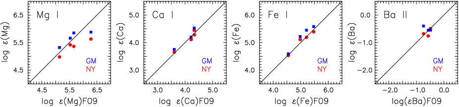
Figure 7.— The abundances log $\epsilon$ from the present work of NY (red circles) and GM (blue squares) vs. those of Feltzing et al. (2009) for elements in common between the two investigations.

The conclusion of this external literature comparison is that the internal accuracy of elemental abundances determinable from spectra of the quality available here is adequately represented by the uncertainties listed in Table 7, while single discordant measures should be treated as provisional.

4. RELATIVE ELEMENT ABUNDANCES

The dependence of relative abundances, [X/Fe], on [Fe/H] for Boötes I is shown in Figure 8 as large red filled circles (NY) connected to large blue filled squares (GM), together with the data for Boo-1137 from Norris et al. (2010c) (as a large red filled circle at [Fe/H] = –3.7). In the top left panel we plot the Boötes I [C/Fe] and [Fe/H] abundances from Norris et al. (2010b) (large filled red circles) and Lai et al. (2011) (large open red circles). For comparison, we also present the abundances for C-normal and C-rich red giants of the Galactic halo (as small filled and open black circles, respectively) from the work of Aoki et al. (2002, 2004), Cayrel et al. (2004), Depagne et al. (2002), François et al. (2007), Fulbright (2000), Ito et al. (2009), Norris et al. (1997), and Spite et al. (2005). Inspection of Figure 8 confirms that, with the exception of the abundances for Boo-119 (at [Fe/H] $\sim$ –3.3) and for Cr I in two other stars, the results of the NY and GM abundance determinations are in agreement, and the uncertainties derived above are a fair estimate of the true error. The figure also gives one the general impression that to first order the abundances of the Boötes I giants follow the trends established by the Galactic halo giants, as we reported earlier for Boo-1137 (Norris et al., 2010c).

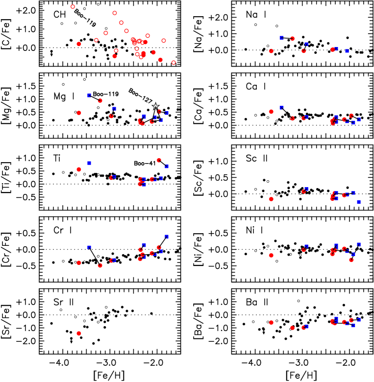
Figure 8.— Relative abundances [X/Fe] vs. [Fe/H] for Boötes I and Galactic halo red giants. (The observed species is identified in each panel, and Ti represents the average of Ti I and Ti II.) In all panels except that at top left, the large blue filled squares represent the abundances of GM, while the large red filled circles stand for those of NY and Boo-1137 (from Norris et al. 2010c) (Results for the same star are connected). In the upper left panel the large filled and open red circles represent the carbon and iron abundances of Norris et al. (2010b) and Lai et al. (2011), respectively, for Boötes I red giants. In all panels the small filled and open black circles represent Galactic halo C-normal and C-rich stars, respectively, from the work of Aoki et al. (2002, 2004), Cayrel et al. (2004), Depagne et al. (2002), François et al. (2007), Fulbright (2000), Ito et al. (2009), Norris et al. (1997), and Spite et al. (2005). In the Mg I panel, the black star presents results for Boo-127 from the work of Feltzing et al. (2009); see Sections 3.5 and 4.1 for discussion of this object.

Comparison with the halo trends identifies two anomalies in the data presented in Figure 8. The first is the large departure of [Ti/Fe] in Boo-41 (at [Fe/H] $\sim$ –1.85) from the trends found in both Boötes I and the halo of the Milky Way. In contradistinction, the [Ti/Fe] values of NY and GM agree well, for both Ti  I and Ti  II. We can offer no explanation for the discrepancy, which is particularly puzzling, since, as we shall see below, Boo-41 is not an outlier when one considers [Ca/Fe], which has the smallest errors by far of the three $\alpha$-elements (Mg, Ca, Ti) observed here.

The second significant discrepancy is between the NY and GM results for Boo-119. For the four species investigated in both analyses – Na, Mg, Ca, and Cr – the absolute differences in $\Delta$[X/Fe] are 0.05, 0.20, 0.41, and 0.54 dex, respectively. We refer the reader to Section 3.3 for the discussion of effects that might lead to differences such as these. Given our conclusion that Boo-119 is a member of the rare CEMP-no class, further observations should be obtained to improve and extend the present results.

4.1. [Mg/Fe] and [Mg/Ca] Enhancements in Boötes I?

There have been a number of reports of significantly non-solar [Mg/Fe] and [Mg/Ca] values in otherwise normal stars in the metal-poor populations of the Galaxy and its satellite galaxies, ranging from [Mg/Ca] = –1.2 in a halo field red giant (Lai et al., 2009) to +0.9 in the Hercules ultra-faint dwarf galaxy (Koch et al., 2008). As noted in Section 3.5, Feltzing et al. (2009) reported [Mg/Fe] $\sim$ +0.7 and [Mg/Ca] $\sim$ +0.7 for Boo-127. We are unable to confirm these results for Boo-127 in the present work. The discrepancy is shown in the [Mg/Fe] panel of Figure 8 where we represent their result as an open star, joined by lines to the present values of NY and GM, both of whom do not find it to have enhanced [Mg/Fe] compared with the Galactic halo trend. We note that we also find [Mg/Ca] = –0.08 (NY) and +0.09 (GM), essentially the solar value. Given the importance of the interpretation of variations in [Mg/Ca] as the signature of enrichment by individual supernovae, confirming an anomalous value requires strong evidence. Here we advocate that our determination of [Mg/Ca] in this star be adopted, unless/until future new data support an anomalous value.

In the [Mg/Fe] panel of Figure 8, we identify the outlier Boo-119, with [Mg/Fe] $\sim+1.0$ ([Mg/Ca] = +0.7). To support the reality of this measurement we present our spectra of the Boötes I giants in the region of the Mg I 5528.4 Å line in Figure 9, where in the lowest panel the Mg I line and two Fe I lines are identified. Inspection of the figure shows that the Mg I line is significantly stronger than the Fe I lines in the spectrum of Boo-119, and in only this star.

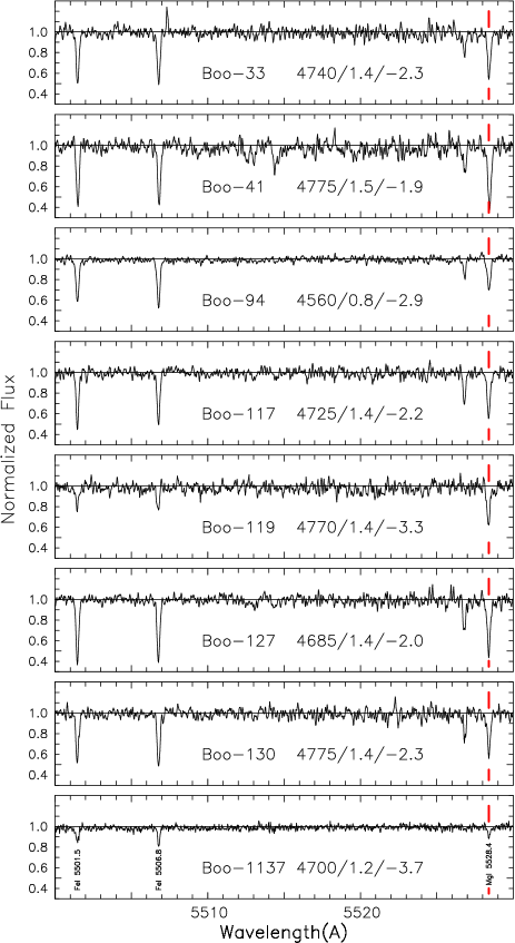
Figure 9.— Spectra of the Boötes I giants in the region of Mg I 5528.4 Å. Three atomic lines are identified in the lowest panel. Note that only in Boo-119 is the Mg I line stronger than the two lines Fe I 5501.5 and 5506.8 Å. Boo-119 is Mg-rich, with [Mg/Fe] = 1.0. Mean adopted atmospheric parameters $T_{\rm eff}$/$\log g$/[Fe/H] are shown in each panel.

Fortuitously, additional abundance information is available for Boo-119: it has also been observed by Lai et al. (2011), who designate it Boo21, and report abundances [Fe/H] = –3.8 and [C/Fe] = +2.2 (this is the C-rich star at top left of the [C/Fe] panel in Figure 8; note that the low-resolution spectra obtained by Lai et al. do not provide abundances of individual $\alpha$-elements). Boo-119 is thus very carbon rich. It also has [Ba/Fe] = –1.0 (according to NY; GM do not measure this feature) and is therefore a CEMP-no star (see Beers & Christlieb 2005 for the definition of terms; as discussed below, the abundances measured in CEMP-no stars most likely reflect those of the interstellar medium (ISM) from which they formed). Mg enhancement is frequently observed in such stars (Masseron et al., 2010; Norris et al., 2012). We therefore conclude that the Mg enhancement we report for Boo-119 is real, and that its C, Mg, and Ba abundances are together consistent with its being a CEMP-no star. Boo-119 joins Segue 1-7 as the second CEMP-no star to be recognized in the Milky Way’s ultra-faint galaxies (cf. Norris et al., 2010a).

4.2. The $\alpha$-elements

The relative abundances of the $\alpha$-elements [Mg/Fe], [Ca/Fe], [Ti/Fe] (= ([Ti I/Fe] + [Ti II/Fe])/2), and [$\alpha$/Fe] (= [Mg/Fe] + [Ca/Fe] + [Ti/Fe])/3) are presented as a function of [Fe/H] in Figure 10, for the stars of the present work (excluding the Mg-enhanced CEMP-no star Boo-119), together with results for Boo-1137 from Norris et al. (2010c). (For the stars in the present work, we have averaged the abundances of NY and GM in Table 7, while for Boo-1137 we have recomputed the $\alpha$-element abundances using only lines from Norris et al. (2010c) having wavelength greater than 4870 Å, in order to reproduce more closely the wavelength coverage of the present investigation.) The data are summarised in Table 9.

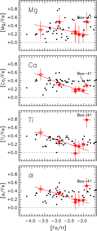
Figure 10.— [$\alpha$/Fe] vs. [Fe/H] for C-normal red giants in Boötes I (filled red stars, this work; open red star, Norris et al., 2010c) and the Galactic halo (small black circles, from Cayrel et al., 2004 and Fulbright, 2000). See text for discussion.

Table 9ADOPTED $\alpha-$ELEMENT ABUNDANCES

Star	[Mg/Fe]	$\sigma$	[Ca/Fe]	$\sigma$	[Ti/Fe]	$\sigma$	[$\alpha$/Fe]	$\sigma$	[Fe/H]	$\sigma$
Boo-33	0.26	0.22	0.14	0.06	$-$0.02	0.17	0.13	0.17	$-$2.32	0.16
Boo-41	0.50	0.22	0.28	0.06	0.78	0.20	0.52	0.18	$-$1.88	0.16
Boo-94	0.49	0.16	0.30	0.06	0.26	0.13	0.35	0.10	$-$2.94	0.16
Boo-117	0.18	0.22	0.20	0.06	0.14	0.13	0.18	0.15	$-$2.18	0.16
Boo-119	1.04	0.22	0.46	0.18	0.80	0.28	0.77	0.15	$-$3.33	0.16
Boo-127	0.17	0.18	0.16	0.05	0.20	0.14	0.18	0.13	$-$2.01	0.16
Boo-130	0.21	0.22	0.19	0.08	0.17	0.16	0.19	0.16	$-$2.32	0.16
Boo-1137	0.30	0.21	0.55	0.14	0.48	0.10	0.44	0.09	$-$3.66	0.11

The relative abundances of the $\alpha$-elements to iron in the seven carbon-normal (i.e., excluding Boo-119) member stars of Boötes I are, with the exception of one outlier in one element, indistinguishable from those of a typical star in the halo of the Milky Way, being $\lesssim 2\sigma$ away from the bulk of the field halo. The outlier is Boo-41, which, as noted above, is significantly more enhanced in Ti than is the bulk of the halo, and indeed is more enhanced than the other member stars of Boötes I. We note for completeness that the four Boötes I stars with [Fe/H] $\sim-2.25$, again excluding Boo-41 from the comparison, have remarkably similar elemental abundances.

We note explicitly one pattern in the $\alpha$-element data which, while of limited statistical significance, is a hint of what one would search for in larger samples of Boötes I stars. If one were to exclude all the abundance data for Boo-41, on the basis of its anomalous Ti abundance, and those data for Boo-119, the CEMP-no star, one sees a clear decrease in the relative abundance of all three elements in the remaining 6 member stars as [Fe/H] increases. The line in each panel of Figure 10 is the least-squares line of best fit, excluding Boo-41. For Mg, Ca, Ti, and $\alpha$ the slopes of the line are –0.115, –0.237, –0.216, –0.189, respectively, while the RMS scatters about the line are 0.105, 0.046, 0.105, and 0.043 dex.

Dependencies of this type are physically plausible, are suggestive of a relatively low star formation rate at the earliest times in this ultra-faint system, and are driven by a contribution of Type Ia supernovae to the chemical enrichment of these elements. Such patterns are seen in the more luminous dwarf spheroidal galaxies, albeit at higher values of [Fe/H], where the higher iron abundance reflects faster enrichment in these larger systems (see, e.g., Tolstoy et al., 2009, their Figure 11).

This digression aside, retention of Boo-41 in our full sample of seven carbon-normal Boötes I stars provides a different picture, with no clear trend in $\alpha$-abundance ratios. Rather, there is a distribution which is, within measurement errors, consistent with having a mean value, and a scatter about that mean, which are similar to those found in the field halo, albeit with the exception of a significant scatter in Ti. If one decided to sub-select the sample of Boötes I stars, one might even argue for the exclusion of Boo-1137, which is presently at significantly larger projected distance from the center than are the other stars (it is at 24 arcmin, the rest within 8 arcmin); this would weaken the case for a smooth decline in elemental ratios as the metallicity increases. Data for a larger sample of Boötes I stars is clearly desirable. That said, the lack of significant scatter in the entirety of the present sample (further quantified in the following section) is itself consistent with a relatively slow early star-formation (and enrichment) rate, since time is required for SNe ejecta from a range of progenitor masses to be created and mixed into the ISM prior to the bulk of star formation.

4.3. Relative-Abundance Dispersions

A critical consideration in seeking to understand the manner in which chemical enrichment occurs in any stellar system is the dispersion of abundance as a function of overall enrichment. To address this issue, we follow Cayrel et al. (2004, their Section 4), who, for element X, determine the linear least squares fit of [X/Fe] as a function of [Fe/H] and measure the dispersion $\sigma$[X/Fe] about that fit.

We restrict the sample for this analysis of scatter to only the six carbon-normal stars analyzed double-blind in this study (thus excluding Boo-119 and Boo-1137). Given the small sample of Boötes I stars and in some cases very few lines of some elements, we have further restricted our focus towards those atomic species for which we can determine relative abundances most accurately. To this end, we included only neutral species, to minimize errors of measurement in [X/Fe], and used only elements for which more than one line has been measured in more than two stars. These conditions are met by Ca I, Ti I, Cr I and Ni I.

Table 10 presents the resulting dispersions, where for each species columns (2) – (5) contain the abundance dispersion, the mean error of measurement, the number of stars, and the mean number of lines measured, from the analysis of NY, while columns (6) – (9) contain the results from the GM analysis. For comparison, we also determined the same parameters from the abundances of Cayrel et al. (2004), for stars having –3.0 $<$ [Fe/H] $<$ –2.0 (the range pertaining to the Boötes I stars under discussion here) and present the results in columns (10) – (13) of the table. We interpret the equality of the observed dispersion and errors of measurement in the Cayrel et al. (2004) data set as indicating that no intrinsic spread has been observed for these elements in halo stars in this abundance range. We also note that the smaller measurement errors of Cayrel et al. (2004) compared with those in the present work are not unexpected, given the higher signal-to-noise of their work ($S/N$ $\sim 200$ per 0.015 Å pixel at 5100 Å) compared with our value of $\sim 30$ per 0.03 Å pixel at 5500 Å.

Table 10RELATIVE-ABUNDANCE DISPERSIONS

Species	$\sigma_{\rm Boo}$	$\sigma_{\rm meas}$	Nstars	$\langle$Nlines$\rangle$	$\sigma_{\rm Boo}$	$\sigma_{\rm meas}$	Nstars	$\langle$Nlines$\rangle$	$\sigma_{\rm Halo}$	$\sigma_{\rm meas}$	Nstars	$\langle$Nlines$\rangle$
	NY	NY	NY	NY	GM	GM	GM	GM	C04	C04	C04	C04
(1)	(2)	(3)	(4)	(5)	(6)	(7)	(8)	(9)	(10)	(11)	(10)	(11)
$[$Ca I/Fe$]$	0.11	0.07	6	8.8	0.08	0.06	6	10.3	0.06	0.07	13	15.8
$[$Ti I/Fe$]$	0.31	0.11	6	4.8	0.27	0.09	6	7.8	0.06	0.05	13	12.9
$[$Cr I/Fe $]$	0.11	0.11	6	4.8	0.21	0.07	6	4.7	0.08	0.07	13	6.9
$[$Ni I/Fe $]$	0.12	0.17	6	2.5	0.12	0.08	6	6.2	0.09	0.09	13	3.0

The data in Table 10 provide no evidence for detection of a spread in elemental ratios at any value of [Fe/H] in Boötes I, with the already noted exception of Ti. Given the differences between the NY and GM analyses, which make clear our quoted values of $\sigma_{\rm meas}$ are estimates, not precision determinations, the observed dispersions are commensurate with the errors of measurement. Quadratic subtraction of these two quantities to produce intrinsic dispersions, at better than the 0.05 – 0.10 dex level, is questionable. Bearing this caveat in mind, we offer the following comments. For Ca, the NY and GM analyses admit intrinsic dispersions of 0.08 and 0.05 dex, respectively. We also recall from the previous section that the average of the NY and GM relative abundances (excluding the outlier Boo-41) yield an observed dispersion in [Ca/Fe] of 0.046 dex. For Ti, the data indicate a dispersion $\sim$0.25 dex, driven largely by the inclusion of the outlier Boo-41 discussed above; exclusion of this object reduces the intrinsic dispersion to $\sim$0.1 dex. For Cr, any intrinsic dispersion is poorly determined, and lies in the range 0.00 – 0.20 dex. Finally, for Ni the more accurate determination of GM suggest a dispersion not larger than 0.1 dex.

For completeness, we note that for the ionized species, which were excluded from consideration by the selection criteria above (i.e. Sc II, Ti II, and Ba II), the mean error of measurement lies in the range 0.19 – 0.24 dex.

4.4. Barium

For the Boötes I giants, the dispersion of [Ba/Fe] in Figure 8 is consistent with that of the Galactic halo. It is interesting to compare the Boötes I data with those of Frebel et al. (2010) for the Com Ber and UMa II ultra-faint dwarf galaxies. For Com Ber at [Fe/H] $\sim-2.5$ the mean barium abundance is $\langle$[Ba/Fe]$\rangle$ $\sim$ –1.8 $\pm$ 0.4, significantly smaller than for Boötes I, for which $\langle$[Ba/Fe]$\rangle$ $\sim$ –0.5 $\pm$ 0.2 – suggestive of a difference in the production efficiency of the heavy-neutron-capture elements between the two systems. For UMa II, on the other hand, one finds $\langle$[Ba/Fe]$\rangle$ $\sim$ –1.0 $\pm$ 0.5, the same to within the errors as that of Boötes I.

We conclude by noting that the Boötes I C-rich star (Boo-119) has a low value of [Ba/Fe], signaling its membership of the CEMP-no class. An important area for future study is the determination of [Ba/Fe] in the four other C-rich stars ([C/Fe] $>$ 0.7) in Figure 8 to constrain more strongly the fraction of CEMP-no stars in the ultra-faint dwarf galaxies.

5. DISCUSSION

5.1. The Properties of Boötes I

Boötes I currently is the only ultra-faint satellite galaxy with a well-defined metallicity distribution derived from medium-resolution spectroscopic observations, plus a significant number of member stars with high-resolution measured abundances of a range of elements, including carbon, across the entire range of [Fe/H] from $\sim-3.5$ to $\sim-2$ dex. The wealth of data for Boötes I allows one to trace chemical evolution at the lowest abundances, with confidence that the stars formed in the same potential well, in a self-enriching system. This is in contrast with the situation for the sample of stars in the Galactic halo field, whose histories and origins are unknown.

Boötes I has a broad metallicity distribution with a well-defined peak, characterized by a mean iron abundance of $-2.6$ dex with dispersion (standard deviation) of 0.4 dex (Norris et al., 2010b; Lai et al., 2011), encompassing stars as iron-poor as $-3.7$ dex. The existence of stars of very low chemical abundances, and the wide range of abundances, make Boötes I fully consistent with being a self-enriched galaxy that had an essentially primordial initial metallicity. The low value of the mean stellar metallicity is consistent with supernovae-driven loss of $\lower 2.15277pt\hbox{$\;\buildrel>\over{\sim}\;$}90\%$ of the initial baryons during star formation and self-enrichment, assuming a normal IMF and standard nucleosynthetic yields during the enrichment (cf. Hartwick, 1976), consistent with the IMF inferred from the elemental abundances of the bulk of the stars. The color-magnitude diagram of Boötes I is that of a metal-poor, exclusively old population (Belokurov et al., 2006; Okamoto et al., 2012), also consistent with early star-formation truncated by gas loss.

The radial-velocity distribution of candidate member stars is offset from that of most field stars, ensuring reliable membership identification. The mass inferred from the kinematics is orders of magnitude larger than the stellar mass (estimated to be $4\times 10^{4}$M_⊙ for an assumed normal IMF (Martin et al., 2008)), and implies dark-matter domination. Scaling from the values given in Table 1 of Walker et al. (2009) to take account of the revised velocity dispersion value noted earlier, the dark-matter mass of Boötes I is $\lesssim 10^{7}$M_⊙, and adopting the half light radius of $\sim 200$pc as a fiducial scalelength, the virial temperature characterizing the potential well is $\sim 3\times 10^{3}$ K: this sets the initial temperature of gas, assuming it is shock-heated as it comes into equilibrium within the dark-matter potential. The high mass-to-light ratio also implies that Boötes I lost $\lower 2.15277pt\hbox{$\;\buildrel>\over{\sim}\;$}90\%$ of its baryons, if the initial value of baryonic to non-baryonic matter were the cosmic value.

The mean mass density of Boötes I, inferred from its internal stellar kinematics is $<\rho>\sim 0.025$ M_⊙ pc^-3, where this value reflects a reduction of a factor of four from the mean density derived in Walker et al. (2009), to correct for the newer and lower value of the central velocity dispersion determined by Koposov et al. (2011). Using this value, the simple assumption of dissipationless collapse of a top-hat spherical density perturbation leads to an estimated virialization redshift $\lower 2.15277pt\hbox{$\;\buildrel>\over{\sim}\;$}10$, consistent with Boötes I having started star formation prior to the completion of reionization.

Although this is well-established as yet only for Boötes I, in general as data improve the ultra-faint dwarf spheroidals are showing abundance distribution functions and inferred stellar age distributions consistent with being surviving examples of the first systems to form stars (e.g. Bovill & Ricotti, 2011; Brown et al., 2012). The ultra-faint galaxies therefore are of critical importance in understanding early star formation and chemical evolution. The massive stars in these systems could well be important sources of the ionizing photons that contributed to reionization.

5.2. Chemical Evolution of Boötes I: Implications from the $\alpha$-elements

The $\alpha$-elements, together with a small amount of iron, are created and ejected by core-collapse supernovae, on timescales of less than $10^{8}$yr after formation of the supernova progenitors. Enhanced (above solar) ratios of [$\alpha$/Fe] are expected in stars formed from gas that is predominantly enriched by these end-points of massive stars. Thus chemical abundances in the stars formed in the first $\lesssim 0.5$ Gyr after star-formation began will reflect the products of predominantly core-collapse supernovae. As has already been noted in the case of the field halo (see also Nissen et al., 1994 and Arnone et al., 2005), a lack of scatter in these element ratios at given [Fe/H] requires that: (i) the stars formed from gas that was enriched by ejecta sampling the mass range of the progenitors of core-collapse supernovae; (ii) the supernova progenitor stars formed with an IMF similar to that of the solar neighborhood today; and (iii) the ejecta from all SNe were efficiently well-mixed.

Both the first and last points set an upper limit on how rapidly star formation could have proceeded, since the star formation regions need to populate the entire massive-star IMF, the stars need sufficient time to all explode, and the gas needs time to mix the ejected enriched material – all before substantial numbers of low-mass stars form.

Our formal full-sample result derived above is that the six carbon-normal stars analyzed here show no evidence for any deviation in the mean value of [$\alpha$/Fe] or any resolved scatter in element ratios, within a limit of $\sim 0.1$ dex, with the exception of a single star, Boo-41, with an anomalous abundance of a single element, Ti. We noted the intriguing possibility that Boo-41 as an outlier star is masking evidence of a resolved steady decline in mean [$\alpha$/Fe] with [Fe/H]. This (possible) decline in the values of [$\alpha$/Fe], as a function of [Fe/H], suggested by the data in Figure 10 could reflect the injection of iron from Type Ia, indicating that the duration of star formation was a time comparable to that for Type Ia SNe to explode and for their ejecta to be incorporated in the next generation, $\lesssim$ 1Gyr. The apparent decline could also simply reflect small number statistics, as noted earlier.

The upper limit in intrinsic scatter of the $\alpha$-element to iron ratios, as a function of iron, that was derived for our six carbon-normal stars in Section 4.3, implies that mixing of the ISM was efficient across the scales probed by the sample. The knowledge that all the stars are members of Boötes I – and presumably formed there – provides a critical piece of information that cannot be ascertained for the field halo, namely the physical scale over which mixing must be efficient. The present sample probes projected distances from the center of Boötes I of several hundred parsecs, and this is the natural scale to adopt.

Type Ia supernovae produce significant amounts of iron, about ten times as much per supernova as core-collapse events, but contribute little to the abundances of the alpha-elements. The ‘Delay Time Distribution’ describing the time between formation of the progenitors and the subsequent Type Ia supernova explosions is model dependent; however this lag cannot be shorter than the lifetime of an 8 M_⊙ star ($\sim 10^{8}$yr). Popular models have a peak rate at intermediate delays ($\sim 10^{9}$ yr), with non-negligible rates at delays of many Gyr, continuing to very late times (e.g. Figure 1 of Matteucci et al., 2009). The iron abundance at which the nucleosynthetic products from Type Ia supernovae are manifest in the next generation of stars depends on the detailed gas physics and the star formation rate, with lower rates allowing the signatures of Type Ia – lower values of [$\alpha$/Fe] – to occur at a lower iron abundance.

Star formation in extremely metal-poor gas in low-mass halos (virial temperature less than $10^{4}$ K so that cooling by atomic hydrogen is not feasible) depends critically on the ionized fraction, as this controls the creation of both molecular hydrogen and the HD molecule, both of which can provide efficient cooling channels (e.g. Johnson & Bromm, 2006). Suffice to say that the cooling is complex, but a low gas temperature may be expected, $T\lesssim 100$ K, with corresponding sound speed in atomic hydrogen of $\sim 2$ km s^-1 (similar to the observed stellar velocity dispersion). Star formation in such systems has been shown to lead to a metal-poor population of stars with a mass function encompassing low masses (Clark et al., 2011). The sound-crossing time may be taken as a characteristic timescale for transport of metals and thus a limit on the mixing timescale. Mixing over the half-light radius of Boötes I then took of order $\sim 10^{8}$ yr. The lack of intrinsic scatter in the $\alpha$-element ratios of stars within the half-light radius then requires a minimum duration of star formation in Boötes I of $\gtrsim 10^{8}$ yr. This is long enough that the progenitor-mass range of core-collapse supernovae should be fully sampled and some Type Ia supernovae may have occurred.

As noted above, the present stellar mass of Boötes I is $\sim 4\times 10^{4}$ M_⊙; a normal stellar IMF implies an initial mass of stars of around a factor of two higher (a locked-up fraction of around 50%, long after star formation ceased). The time-averaged star-formation rate, using the duration of $10^{8}$ yr from above, is then less than 0.001 M_⊙/yr. This is small in absolute terms, but the one-dimensional velocity dispersion of Boötes I is only $\sim 3~{}$km s^-1, well below the critical minimum value for retention of gas in idealized models of supernova feedback from star-formation on a crossing time (Wyse & Silk, 1985).

A lack of scatter in the $\alpha$-elemental abundance ratios also requires that the well-sampled IMF of core-collapse supernova progenitors be invariant over the range of time and/or iron abundance. As discussed by Wyse & Gilmore (1992) and Nissen et al. (1994), and revisited in Ruchti et al. (2011), the value of the ratios of the $\alpha$-elements to iron during the regimes where core-collapse supernovae dominate the chemical enrichment is a sensitive measure of the masses of the progenitors of the supernovae. This is most simply expressed as a constraint, from the scatter, on the variation in slope of the massive-star IMF, assuming that the ratios reflect IMF-averaged yields. A scatter of $\pm 0.02$ constrains the variation in IMF slope to be $\pm 0.2$ (Ruchti et al., 2011, their Figure 30). The overall agreement between the values of the elemental abundances in Boötes I stars and in the field halo implies the same value of the massive-star IMF that enriched the stars in each of the two samples, though our formal limit on this IMF slope is only agreement within a slope range of $\pm 1$.

5.3. Chemical Evolution of Boötes I and CEMP Stars: Implications from Carbon Abundances

Boötes I and the Galactic halo display a large spread in carbon abundance at lowest metallicity. At [Fe/H] = –3.5, for example, both exhibit a range of $\Delta$[C/Fe]$\sim 2-3$ dex (see, e.g., the top-left panel of Figure 8). Further, the fraction of CEMP stars in Boötes I relative to that of giants in the halo in the range –4 $<$ [Fe/H] $<$ –2 is $\sim$ 0.2, similar to that found in the Galactic halo. That said, while the halo CEMP class comprises several subclasses (CEMP-r, -r/s, -s, -no; see the classification of Beers & Christlieb, 2005) little is known about the situation for the dwarf spheroidal and ultra-faint satellites. As discussed in Section 4.1, in these systems data of quality sufficient to determine their subclass exist for only two CEMP stars. These are Boo-119 and Segue 1-7, both of which belong to the CEMP-no subclass. Both also have [Fe/H] $\sim-3.5$, consistent with the finding that in the Galactic halo only CEMP-no stars exist below [Fe/H[ $\sim$ –3.2 (see, e.g., Aoki, 2010 and Norris et al., 2012).

It should be noted that the most iron-poor star currently known in Boötes I, Boo-1137, is not carbon-enhanced. Carbon-enhanced and “carbon-normal” stars co-exist at the same low iron abundance within the same system. The recent discovery by Caffau et al. (2011, 2012) of an ultra metal-poor ([Fe/H]_1D,LTE = –4.7, [Fe/H]_3D,NLTE = –4.9) low-mass star, in the Milky Way halo with no carbon enhancement ([C/Fe] $<$ +0.9) is further evidence that carbon enhancement is not required for very low-iron abundance gas to cool and form low-mass stars.

CEMP stars that exhibit high values of neutron-capture $s-$process elements (the CEMP-s stars) show a high incidence of binarity (e.g. Lucatello et al., 2005) and are probably carbon-rich due to the accretion of enriched material from an asymptotic giant branch companion. As shown by Norris et al. (2012), however, the binary statistics for CEMP-no stars are decidedly different from those of CEMP-s stars, offering little support, currently, for a large percentage of CEMP-no stars belonging to binary systems. CEMP-no stars are more likely to have formed from gas enriched by non-standard (“mixing and fallback” supernovae (Umeda & Nomoto, 2003; Iwamoto et al., 2005), or by the winds from rapidly-rotating massive stars (Meynet et al., 2006, 2010). Unusually elevated magnesium is frequently also found in such stars (Aoki et al., 2002; Norris et al., 2012), with presumably both the magnesium and carbon over-abundances reflecting the yields of the very first generation of supernovae or massive stars. The presence of CEMP-no stars in the two ultra-faint dwarf galaxies is strong evidence for their self-enrichment from primordial material. It provides an opportunity to consider the evolutionary history of the extremely carbon-enriched, Fe-poor ISM gas.

The important additional information we consider here is that CEMP-no stars are not found at [Fe/H] $\lower 2.15277pt\hbox{$\;\buildrel>\over{\sim}\;$}-2.5$, either in the field halo (Aoki, 2010) or in dwarf spheroidal galaxies (Norris et al., 2010b; Lai et al., 2011). Given the amplitude of the [C/Fe] and [Mg/Fe] values in CEMP-no stars, one must also explain why stars are not found with intermediate C and Mg excesses at higher [Fe/H]. Apparently the highly C- and Mg-enriched ISM does not survive to mix with “normal” enriched ISM and form more stars with moderate CEMP-no enrichment. Rather, the cooling efficiency of the highly carbon-enriched material must be sufficiently great that all of it cools and forms (the surviving) low-mass stars before there is time to mix this material with “normal” SNe ejecta.

This is illustrated in Figure 11, which shows [C/Fe] vs. [Fe/H] for stars in the Boötes I dwarf galaxy, based on two samples: filled circles represent data of Norris et al. (2010c), with the exception of the CEMP-no star Boo-119, which has been plotted adopting the carbon abundance from Lai et al. (2011) and the iron abundance from the present work, while open circles and upper limits represent data from Lai et al. (2011). The smooth curve starts at Boo-119, and tracks the expected evolution due to addition of enriched gas in which carbon and iron are in the solar ratio, consistent with normal core-collapse supernovae and the value of the [C/Fe] ratio for the bulk of field halo stars. This curve skims along the top of the distribution for Boötes I and clearly fails to explain the bulk of the “carbon-normal” population. This suggestion is supported also by the data for the Segue 1 ultra-faint system, for which the available sample having carbon abundances is limited to three stars (Norris et al., 2010b, a), shown as filled triangles in Figure 11. The analogous carbon-dilution curve for Segue 1, starting at the CEMP-no star Segue 1-7 at ([C/Fe], [Fe/H]) = (+2.3, –3.5) (Norris et al., 2010a), would also fail to explain the carbon-normal stars in this system. We conclude that there appears to be two distinct channels of enrichment, one creating CEMP-no stars, and the other creating carbon-normal stars. Both channels operate at low iron abundance, [Fe/H] $\lesssim-2.5$, but only the carbon-normal channel remains at higher [Fe/H]. Norris et al. (2012) reached the same conclusion from their analysis of the abundance patterns of Galactic halo C-rich stars with [Fe/H] $<$ –3.1.

Figure 11.— [C/Fe] vs. [Fe/H] for stars in the Boötes I dwarf galaxy (filled circles represent data of Norris et al. (2010b), with the exception of the CEMP-no star Boo-119, which has been plotted adopting the carbon abundance from Lai et al. (2011) and the iron abundance from the present work; open circles and upper limits represent data from Lai et al. (2011)) and for the Segue 1 dwarf galaxy (filled triangles, data from Norris et al. (2010b, a)). The smooth curve starts at Boo-119, and tracks the expected evolution due to continuing star formation in gas to which carbon and iron are added in the solar ratio, consistent with normal core-collapse supernovae. As discussed in the text, the data suggest two distinct channels of enrichment, one carbon-rich, and one carbon-normal.

The inability to form the bulk of the carbon-normal stars by an earlier population of CEMP-no stars is most clear in the case of individual self-enriching systems, as opposed to a sample of stars in the field halo with unknown, and likely varied, formation sites. The available sample of field halo stars is shown in Figure 12, where the analysis has been extended to include [Mg/Fe] (see Norris et al., 2012 for a full description of these data). Dilution tracks can be found that start at observed values and pass through the bulk of the stars. However, there is no guarantee that stars so-connected were ever part of the same self-enriching system.

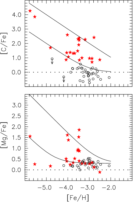
Figure 12.— [C/Fe] and [Mg/Fe] vs. [Fe/H] for Galactic halo CEMP-no stars (star symbols, from Norris et al. 2012) and C-normal stars (circles, from Cayrel et al., 2004 and Caffau et al., 2011). The lines represent dilution trajectories, as C-rich and Mg-rich material produced at the earliest times is mixed with C-normal and Mg-normal halo material. As [Fe/H] increases to –2.5, early C-rich and Mg-rich signatures are no longer evident. See text for discussion.

A comparison between the distributions and carbon-dilution tracks in Figures 11 and 12 shows the power of knowing that the stars in the Boötes I sample are part of a self-enriching system and therefore can be connected by a chemical evolutionary path: choosing a different starting point for the carbon-dilution track in Figure 11 could provide values of [C/Fe] and [Fe/H] that better match those of the bulk of the stars. Indeed, material with an initial [C/Fe] of the same value as for Boo-119, but a factor of a hundred lower iron abundance, would, after dilution by material with solar carbon-to-iron, pass through the locus of the “carbon-normal” stars in Boötes I at [Fe/H] $\lower 2.15277pt\hbox{$\;\buildrel>\over{\sim}\;$}-3$. The challenge would be to find the evidence that a sufficient population of such precursers existed. We can robustly state that with the current knowledge of stars in Boötes I there is no direct chemical evolution track (assuming standard yields of carbon and iron) between the CEMP-no star and the “carbon-normal” stars.

A schematic diagram of the processes underlying the [C/Fe] patterns associated with these two paths is given in Figure 13. This shows, for illustrative purposes, four stars (or star-forming events) in the “CEMP-no” path, denoted by star symbols, while the “normal” path lies along the blue shaded area. The three panels indicate different aspects of enrichment in which we propose that the two paths diverge: the first is [C/Fe] versus [Fe/H], just discussed above; the second is [C/Fe] versus time since the onset of star formation, indicating that star formation of “CEMP-no” stars is initiated prior to the “normal” branch, but may overlap somewhat in time before disappearing; and the third shows [C/Fe] versus mixing length in the ISM. The CEMP-no stars form rapidly out of gas enriched by only one generation of supernovae and likely prior to the onset of good mixing. This results in a small mixing length, spatial inhomogeneity and a large scatter in elemental abundance ratios.

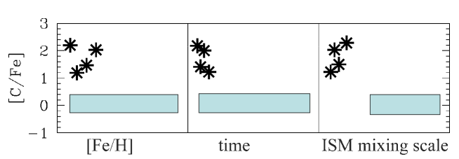
Figure 13.— Schematic illustration of (i) (left panel) the different iron abundance regimes of the two carbon-enrichment channels; (ii) (middle panel) the different timescales since the onset of star-formation applying to the two separate enrichment channels and (iii) (right panel) the two different spatial scales over which nucleosynthetic material was mixed. The star symbols indicate the CEMP-no channel, while the blue band indicates the carbon-normal channel.

This scenario requires that the gas within which the CEMP-no stars form can cool and be locked up in low-mass stars very rapidly, and with high efficiency, so that material with this abundance pattern is removed from the system at early times. Several models of the formation of very metal-poor low-mass stars have appealed to enhanced cooling due to carbon (e.g. review of Bromm & Larson, 2004). It may well be that the CEMP-no material resulted from a very small number of (Population III?) supernovae.

6. SUMMARY

We have analyzed UVES spectra of seven red giant members of Boötes I, and re-analyzed our previous UVES study of an eighth member. The stars cover the range in [Fe/H] from –3.7 to –1.9, and include a CEMP-no star with [Fe/H]= –3.33.

We implemented a double-blind analysis strategy to ensure the most reliable feasible determination of the measuring errors with which elemental abundances could be determined. We did this since the analysis of elemental abundances in low-mass stars in ultra-faint dwarf galaxies provides unique insight into early star formation and chemical enrichment. These systems are inferred to be very dark-matter dominated, are of extremely low surface brightness, with low stellar mass, and have a uniformly old stellar population.

Our elemental abundances are formally consistent with a halo-like distribution, with enhanced mean [$\alpha$/Fe] and at most small scatter about the mean. This is in accord with the high-mass low-metallicity stellar IMF in this very low density system being indistinguishable from the present-day solar neighborhood value. We do find one star with apparently very high [Ti/Fe] abundance, while we also find no support for a previously published high [Mg/Fe] value for another of our stars. We see marginal hints of a decline in [$\alpha$/Fe] with [Fe/H] if we exclude the high-Ti abundance star. Further observations are needed to examine this tentative result.

Our metallicity and elemental abundance data show that Boötes I has evolved as a self-enriching star-forming system, from essentially primordial initial abundances. This allows us uniquely to investigate the place of CEMP-no stars in a chemically evolving system, as well as to limit the timescale of star formation in this ultra-faint dSph. Both the low elemental abundance scatter and the hint of a decline in [$\alpha$/Fe] require low star formation rates, allowing time for SNe ejecta to be created and mixed over the large spatial scales relevant to Boötes I. This is further evidence that Boötes I survived as a self-enriching star-forming system from very early times.

In that context we consider the implications of the existence of CEMP-no stars at very low values of [Fe/H], and the absence of any stars with lesser CEMP-no enhancements at higher [Fe/H] – a situation which is consistent with knowledge of CEMP-no stars in the Galactic field. We show that this observation requires there are two enrichment paths at very low metallicities: CEMP-no and “carbon-normal”.

References

- Abazajian et al. (2009) Abazajian, K. N., Adelman-McCarthy, J. K., Agüeros, M. A., et al. 2009, ApJS, 182, 543
- Alvarez & Plez (1998) Alvarez, R., & Plez, B. 1998, A&A, 330, 1109
- Aoki (2010) Aoki, W. 2010, in IAU Symposium, Vol. 265, IAU Symposium, ed. K. Cunha, M. Spite, & B. Barbuy, 111
- Aoki et al. (2004) Aoki, W., Norris, J. E., Ryan, S. G., et al. 2004, ApJ, 608, 971
- Aoki et al. (2002) Aoki, W., Norris, J. E., Ryan, S. G., Beers, T. C., & Ando, H. 2002, ApJ, 576, L141
- Arnone et al. (2005) Arnone, E., Ryan, S. G., Argast, D., Norris, J. E., & Beers, T. C. 2005, A&A, 430, 507
- Asplund et al. (2005) Asplund, M., Grevesse, N., & Sauval, A. J. 2005, in Astronomical Society of the Pacific Conference Series, Vol. 336, Cosmic Abundances as Records of Stellar Evolution and Nucleosynthesis, ed. T. G. Barnes, III & F. N. Bash, 25
- Asplund et al. (2009) Asplund, M., Grevesse, N., Sauval, A. J., & Scott, P. 2009, ARA&A, 47, 481
- Asplund et al. (2000) Asplund, M., Nordlund, Å., Trampedach, R., Allende Prieto, C., & Stein, R. F. 2000, A&A, 359, 729
- Beers & Christlieb (2005) Beers, T. C., & Christlieb, N. 2005, ARA&A, 43, 531
- Belokurov et al. (2006) Belokurov, V., Zucker, D. B., Evans, N. W., et al. 2006, ApJ, 647, L111
- Bensby et al. (2009) Bensby, T., Johnson, J. A., Cohen, J., et al. 2009, A&A, 499, 737
- Bergemann (2011) Bergemann, M. 2011, MNRAS, 413, 2184
- Bovill & Ricotti (2011) Bovill, M. S., & Ricotti, M. 2011, ApJ, 741, 18
- Bromm & Larson (2004) Bromm, V., & Larson, R. B. 2004, ARA&A, 42, 79
- Brown et al. (2012) Brown, T. M., Tumlinson, J., Geha, M., et al. 2012, ApJ, 753, L21
- Caffau et al. (2011) Caffau, E., Bonifacio, P., François, P., et al. 2011, Nature, 477, 67
- Caffau et al. (2012) —. 2012, A&A, 542, A51
- Castelli & Kurucz (2003) Castelli, F., & Kurucz, R. L. 2003, in IAU Symposium, Vol. 210, Modelling of Stellar Atmospheres, ed. N. Piskunov, W. W. Weiss, & D. F. Gray, A20
- Cayrel et al. (2004) Cayrel, R., Depagne, E., Spite, M., et al. 2004, A&A, 416, 1117
- Clark et al. (2011) Clark, P. C., Glover, S. C. O., Klessen, R. S., & Bromm, V. 2011, ApJ, 727, 110
- Coelho et al. (2005) Coelho, P., Barbuy, B., Meléndez, J., Schiavon, R. P., & Castilho, B. V. 2005, A&A, 443, 735
- Cottrell & Norris (1978) Cottrell, P. L., & Norris, J. 1978, ApJ, 221, 893
- Dall’Ora et al. (2006) Dall’Ora, M., Clementini, G., Kinemuchi, K., et al. 2006, ApJ, 653, L109
- Demarque et al. (2004) Demarque, P., Woo, J.-H., Kim, Y.-C., & Yi, S. K. 2004, ApJS, 155, 667
- Depagne et al. (2002) Depagne, E., Hill, V., Spite, M., et al. 2002, A&A, 390, 187
- Fellhauer et al. (2008) Fellhauer, M., Wilkinson, M. I., Evans, N. W., et al. 2008, MNRAS, 385, 1095
- Feltzing et al. (2009) Feltzing, S., Eriksson, K., Kleyna, J., & Wilkinson, M. I. 2009, A&A, 508, L1
- François et al. (2007) François, P., Depagne, E., Hill, V., et al. 2007, A&A, 476, 935
- Frebel et al. (2010) Frebel, A., Simon, J. D., Geha, M., & Willman, B. 2010, ApJ, 708, 560
- Fulbright (2000) Fulbright, J. P. 2000, AJ, 120, 1841
- Gilmore et al. (2007) Gilmore, G., Wilkinson, M. I., Wyse, R. F. G., et al. 2007, ApJ, 663, 948
- Gustafsson et al. (1975) Gustafsson, B., Bell, R. A., Eriksson, K., & Nordlund, A. 1975, A&A, 42, 407
- Hartwick (1976) Hartwick, F. D. A. 1976, ApJ, 209, 418
- Ito et al. (2009) Ito, H., Aoki, W., Honda, S., & Beers, T. C. 2009, ApJ, 698, L37
- Iwamoto et al. (2005) Iwamoto, N., Umeda, H., Tominaga, N., Nomoto, K., & Maeda, K. 2005, Science, 309, 451
- Johnson & Bromm (2006) Johnson, J. L., & Bromm, V. 2006, MNRAS, 366, 247
- Koch et al. (2008) Koch, A., McWilliam, A., Grebel, E. K., Zucker, D. B., & Belokurov, V. 2008, ApJ, 688, L13
- Koposov et al. (2011) Koposov, S. E., Gilmore, G., Walker, M. G., et al. 2011, ApJ, 736, 146
- Kupka et al. (2000) Kupka, F. G., Ryabchikova, T. A., Piskunov, N. E., Stempels, H. C., & Weiss, W. W. 2000, Baltic Astronomy, 9, 590
- Kurucz (1993a) Kurucz, R. 1993a, ATLAS9 Stellar Atmosphere Programs and 2 km/s grid. Kurucz CD-ROM No. 13. Cambridge, Mass.: Smithsonian Astrophysical Observatory
- Kurucz (1993b) —. 1993b, SYNTHE Spectrum Synthesis Programs and Line Data. Kurucz CD-ROM No. 18. Cambridge, Mass.: Smithsonian Astrophysical Observatory
- Lai et al. (2011) Lai, D. K., Lee, Y. S., Bolte, M., et al. 2011, ApJ, 738, 51
- Lai et al. (2009) Lai, D. K., Rockosi, C. M., Bolte, M., et al. 2009, ApJ, 697, L63
- Lemasle et al. (2007) Lemasle, B., François, P., Bono, G., et al. 2007, A&A, 467, 283
- Lucatello et al. (2005) Lucatello, S., Tsangarides, S., Beers, T. C., et al. 2005, ApJ, 625, 825
- Martin et al. (2008) Martin, N. F., de Jong, J. T. A., & Rix, H.-W. 2008, ApJ, 684, 1075
- Martin et al. (2007) Martin, N. F., Ibata, R. A., Chapman, S. C., Irwin, M., & Lewis, G. F. 2007, MNRAS, 380, 281
- Masseron et al. (2010) Masseron, T., Johnson, J. A., Plez, B., et al. 2010, A&A, 509, A93
- Matteucci et al. (2009) Matteucci, F., Spitoni, E., Recchi, S., & Valiante, R. 2009, A&A, 501, 531
- Meléndez & Barbuy (2009) Meléndez, J., & Barbuy, B. 2009, A&A, 497, 611
- Meynet et al. (2006) Meynet, G., Ekström, S., & Maeder, A. 2006, A&A, 447, 623
- Meynet et al. (2010) Meynet, G., Hirschi, R., Ekstrom, S., et al. 2010, A&A, 521, A30
- Monaco et al. (2011) Monaco, L., Saviane, I., Correnti, M., Bonifacio, P., & Geisler, D. 2011, A&A, 525, A124
- Muñoz et al. (2006) Muñoz, R. R., Carlin, J. L., Frinchaboy, P. M., et al. 2006, ApJ, 650, L51
- Nissen et al. (1994) Nissen, P. E., Gustafsson, B., Edvardsson, B., & Gilmore, G. 1994, A&A, 285, 440
- Norris et al. (2008) Norris, J. E., Gilmore, G., Wyse, R. F. G., et al. 2008, ApJ, 689, L113
- Norris et al. (2010a) Norris, J. E., Gilmore, G., Wyse, R. F. G., Yong, D., & Frebel, A. 2010a, ApJ, 722, L104
- Norris et al. (1997) Norris, J. E., Ryan, S. G., & Beers, T. C. 1997, ApJ, 488, 350
- Norris et al. (2001) —. 2001, ApJ, 561, 1034
- Norris et al. (2010b) Norris, J. E., Wyse, R. F. G., Gilmore, G., et al. 2010b, ApJ, 723, 1632
- Norris et al. (2012) Norris, J. E., Yong, D., Bessell, M. S., et al. . 2012, ApJ, submitted
- Norris et al. (2010c) Norris, J. E., Yong, D., Gilmore, G., & Wyse, R. F. G. 2010c, ApJ, 711, 350
- Okamoto et al. (2012) Okamoto, S., Arimoto, N., Yamada, Y., & Onodera, M. 2012, ApJ, 744, 96
- Pasquini et al. (2002) Pasquini, L., Avila, G., Blecha, A., et al. 2002, The Messenger, 110, 1
- Pietrinferni et al. (2006) Pietrinferni, A., Cassisi, S., Salaris, M., & Castelli, F. 2006, ApJ, 642, 797
- Ruchti et al. (2011) Ruchti, G. R., Fulbright, J. P., Wyse, R. F. G., et al. 2011, ApJ, 737, 9
- Sbordone et al. (2004) Sbordone, L., Bonifacio, P., Castelli, F., & Kurucz, R. L. 2004, Memorie della Societa Astronomica Italiana Supplementi, 5, 93
- Sneden (1973) Sneden, C. 1973, ApJ, 184, 839
- Sobeck et al. (2011) Sobeck, J. S., Kraft, R. P., Sneden, C., et al. 2011, AJ, 141, 175
- Spite et al. (2005) Spite, M., Cayrel, R., Plez, B., et al. 2005, A&A, 430, 655
- Tolstoy et al. (2009) Tolstoy, E., Hill, V., & Tosi, M. 2009, AR&AA
- Umeda & Nomoto (2003) Umeda, H., & Nomoto, K. 2003, Nature, 422, 871
- Walker et al. (2009) Walker, M. G., Mateo, M., Olszewski, E. W., et al. 2009, ApJ, 704, 1274
- Wolf et al. (2010) Wolf, J., Martinez, G. D., Bullock, J. S., et al. 2010, MNRAS, 406, 1220
- Wyse & Gilmore (1992) Wyse, R. F. G., & Gilmore, G. 1992, AJ, 104, 144
- Wyse & Silk (1985) Wyse, R. F. G., & Silk, J. 1985, ApJ, 296, L1
- Yong et al. (2008) Yong, D., Lambert, D. L., Paulson, D. B., & Carney, B. W. 2008, ApJ, 673, 854