The joint use of the tangential electric field and surface Laplacian in EEG classification

Abstract

We investigate the joint use of the tangential electric field and the surface Laplacian derivation as a method to improve the classification of EEG signals. We considered five classification tasks to test the validity of such approach. In all five tasks, the joint use of the components of the tangential electric field and the surface Laplacian outperformed the scalar potential. The smallest effect occurred in the classification of a mental task, wherein the average classification rate was improved by 0.5 standard deviations. The largest effect was obtained in the classification of visual stimuli and corresponded to an improvement of 2.1 standard deviations.

Introduction

Advanced techniques of analysis and interpretation of the EEG signals have grown substantially over the years, with special attention directed to the problems of low spatial resolution and the choice of physical reference. Performing the surface Laplacian differentiation of scalp potentials has proved to be an efficient method to address both issues (Hjorth, 1975; Perrin et al, 1989; He and Cohen, 1992; He et al, 1993; Babiloni et al, 1995; Yao, 2002; Nunez and Srinivasan, 2006). The surface Laplacian operation is reference-free and many studies have suggested that it provides a more accurate representation of dura-surface potentials than conventional topography (Nunez and Pilgreen, 1991; Nunez et al, 1991; Nunez and Westdorp, 1994; Nunez et al, 1994; Srinivasan et al, 1996; Nunez and Srinivasan, 2006). Motivated by this observation, numerous experimental studies of both clinical and theoretical interest have been successfully conducted, such as those of Babiloni et al (1999, 2000, 2001, 2002); Chen et al (2005); Besio et al (2006); Kayser and Tenke (2006a, b); Koka and Besio (2007); Bai et al (2008); Besio et al (2009).

In physical terms, the surface Laplacian of the scalp potential is a measure of local effects of geometry and boundary conditions on the normal component of the underlying current density. This follows directly from the quasistatic continuity of the current density, which implies that any change in flux normal to a surface causes a lateral divergence of flow lines, which may be expressed mathematically as the surface Laplacian of the surface potential. This relationship between the surface Laplacian of the potential and the normal component of the current density results in a spatial filtering property that is responsible for the majority of practical applications of the Laplacian technique. But unless reliable information is available about the physical process underlying the EEG, relying exclusively on the behavior of the normal component of the current density may imply the neglect of potentially valuable information encoded in other spatial components. This observation was a compelling reason to undertake the present work. Thus, in our approach we jointly consider the surface Laplacian of the scalp potential and the tangential components of the scalp electric field to classify EEG signals.

The rationale for this combination is that the electric field is also locally related to the current density by Ohm’s law. Each spatial component of the electric field expresses the (negative) rate of change of the scalar potential in that direction, but because the EEG is only recorded along the scalp, we cannot estimate the field component normal to the scalp surface directly from the data. The use of the surface Laplacian to represent this spatial component is not new in the literature. For instance, He et al (1995) discussed the physical existence of the normal component of the electric field just out of the body surface and used its analytic relationship with the surface Laplacian of the potential to construct a surface-charge model to represent bioelectrical sources inside the body. In the Appendix, we use similar considerations to explain the connection between these quantities at electrode sites on a spherical scalp model.

All computations in our work were performed by means of regularized splines on the sphere. We evaluated the practical effect of the joint approach on five classification tasks, derived from experiments on language, visual stimuli, and a mental task. The results in terms of effect sizes showed an optimistic prospect for further developments and applications.

Methods

Experimental Procedures

All data used in our study were previously obtained in our laboratory as part of experiments on language, vision, and imagination. We label such experiments as Exp. I, Exp. II, and Exp. III, and the subjects who took part in them as S1, S2, S3, $\cdots$, but S1 of Exp. I was not necessarily the same as S1 of Exp. II, and so on. Exp. I encompassed three distinct classification tasks and Exp. II and III one classification task each.

Exp. I: 32 consonant-vowel syllables

This experiment emerged from Rui Wang’s doctoral work (Wang, 2011) and is described in detail in Wang et al (2012), to which the reader is referred for further details. The focus was on the identification of brain patterns related to listening to a set of English phonemes having traditional phonological features of consonants (voicing, continuant, and place of articulation) and vowels (height and backness). The stimuli consisted of the sounds of 32 phonemes (8 consonants $\times$ 4 vowels) formed from pairwise combinations of the consonants /p/, /t/, /b/, /g/, /f/, /s/, /v/, /z/, and the vowels /i/ (as in meet), /ï¿œ/ (cat), /u/ (soon), and /a/ (spa). These vowels were selected also for being maximally separated in the American-English vowel space, which presumably facilitates classification. All phonemes were uttered by a male native speaker of English and recorded in audio files at 44.1 kHz sampling rate. Each syllable was repeated 7 times to produce a variation of pronunciation as commonly occurs in human languages. This resulted in a total of $7\times 32=224$ audio files for presentation.

Four adult subjects (S1-S4), 1 male, participated in this experiment, all reporting no history of hearing problems. The auditory stimuli were presented to participants in random order via a stereo computer speaker. Each participant was instructed to listen carefully to the sounds and try to comprehend them, but no response was required. The stimulus presentations were grouped into multiple sessions of 896 trials (4 repetitions of 224 sounds at random). The trial length, measured from the onset of one stimulus to the onset of the next, had 1,000 ms duration, so that each session lasted approximately 15 min. There was a short break after each block of 56 trials, and the participant could control the length of the break by pressing the spacebar. The number of trials collected from the participants were: 7,168 (S1), 3,584 (S2), 6,272 (S3), and 4,480 (S4).

EEG signals were recorded at 1,000 Hz sampling rate, using a 128-channel Geodesic Sensor Net (Figure 1) on EGI’s Geodesic EEG system 300. There were 124 monopolar channels with a common reference Cz and 2 bipolar reference channels for eye movements.

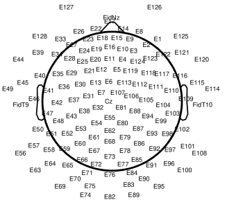
Figure 1: Electrode montage used in Exp. I.

Exp. II: 9 shape-color images

In this experiment researchers from our Lab investigated the brainwave representation of nine two-dimensional images, formed by pairwise combinations of three geometric shapes (circle, square, and triangle) and three colors (red, green, and blue). These images were presented to participants on a 17-inch LED computer screen using the commercial software Presentation. All shapes had approximately the same area of 100 cm², and the physical luminosity was adjusted for each object and color to appear the same at 60 cm from the screen, but no attempt was made to adjust images to each participant, such that the subjective perception of luminosity was the same for all colors and each participant. The distance from the participant’ eyes to the screen was approximately 60 cm and the visual angle was 2.3–3.3^∘. Each presentation lasted 300 ms and was followed immediately by an interval of 700 ms, during which a fixation cross (‘$+$’) was shown at the center of a blank screen. A stimulus appeared randomly and with equal probability every 1,000 ms.

Seven adults (S1-S7), 3 female, agreed to participate in this experiment, all having normal or corrected to normal vision. Participants were instructed to remain relaxed and motionless, and to keep eyes fixed at the center of the screen during presentations. They were seated comfortably on a chair in a dimly lit sound-attenuated booth and responded to 2,700 trials time-locked to stimulus presentations. The presentations were divided in blocks of 20 trials and the participant could control the duration of the breaks via the spacebar. Halfway through the experiment a modified break message was displayed informing the participant that the experiment had passed its halfway point.

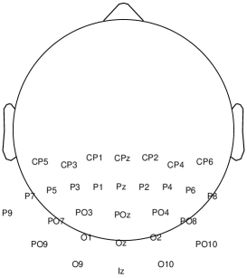
Figure 2: Electrode montage used in Experiment II.

Exp. III: 2-class imagery task

The third experiment was previously described in Carvalhaes et al (2009) and Carvalhaes and Suppes (2011). Eleven participants (S1-S11) were randomly presented on every other trial either a visual “stop” sign, flashed on a 17-inch LED computer screen, or the sound of the English word “go”, via computer speaker. The “go” sound was uttered by a male native speaker of English and recorded in an audio-isolated cabin using a professional microphone interfaced with a computer via a Sound Blaster II (Creative Labs) sound card at 44.1 kHz sampling rate (24 bits). Stimuli were delivered using the Presentation software. The “go” sound was delivery via high fidelity PC speakers at the level of normal conversation. Each stimulus presentation lasted 300 ms, and was followed by a period of 700 ms of blank screen. Immediately after this period a fixation cross (‘$+$’) was shown at the center of the screen for 300 ms.

Eleven subjects participated in this experiment, all adults reporting normal vision and normal hearing. They were comfortably seated in a chair at a distance of approximately 60 cm from a computer screen and 100 cm from the speaker. For one group (S1-S7) the participants were instructed to form a vivid mental image of the stimulus previously presented, for another group (S8-S11) they were asked to form a mental image of the alternative stimulus, i.e., if the last stimulus was the “stop” sign, then they should imagine the “go” sound, and vice versa. Participants’ imagining was followed by another 700 ms of blank screen, after which the trial ended. A single session of 600 trials was recorded for each participant. The session was divided into thirty 20-trial blocks, with regular breaks controlled by participants via the spacebar. Each trial lasted 2,000 ms, but only the last 1,000 ms of each trial corresponding to the imagination task was used for our analysis.

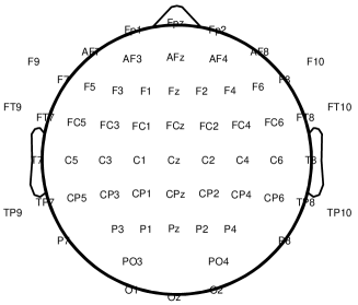
Figure 3: Electrode montage used in Experiment III.

Data collection and preprocessing

Data collection started after participants were given the opportunity to practice the required tasks. The recording apparatus changed from one experiment to another. Exp. I was carried out using EGI’s Geodesic EEG system with 128 monopolar channels referenced to the vertex electrode (Cz) and with a ground electrode placed on the forehead (also for Exp II and III). The electrode locations for this experiment are illustrated in Figure 1. In Exp. II signals were recorded using a 32-channel NeuroScan system with linked earlobe reference (Ag–AgCl electrodes). Due to the low number of channels available on this device – and in view of the need for a reasonable density of electrodes to accurately estimate the electric field in the region of interest V1 (Mikkulainen, 2005) – the measurement electrodes were all placed in the back part of the head, as depicted in Figure 2. We remark that there was no particular reason for choosing P9 instead of P10 in this montage. The electrode distribution was asymmetric and P10 was not included as well just because of the small number of channels that were available to perform this experiment. Exp. III used a 64-channel Neuroscan system, following the 5% system of Oostenveld and Praamstra (2001), but not including electrodes Nz, AF1, AF2, AF5, AF6, T9, T10, P9, P5, P6, P9, P10, PO, or I; the reference being as in Exp. II. Figure 3 shows the electrode distribution for this experiment.

The signals were passed through a band-pass filter in the range 0.1-300 Hz plus a 60 Hz notch filter, and digital conversion was performed at a 1 kHz sampling rate. To reduce features, we carried out offline decimation at 16:1 ratio, thus setting the Nyquist frequency at 31.25 Hz. Additionally, we removed unwanted low-frequency components by applying a high-pass filter of 1 Hz. Finally, we mathematically referenced the decimated signals to the average reference voltage to reduce biases in the analysis of the potential distribution (Bertrand et al, 1985; Murray et al, 2008). This step had no effect on the tangential field and the surface Laplacian derivation, for they are reference-free quantities (He et al, 1993, 1995; Nunez and Srinivasan, 2006).

The signals were visually inspected, but no trial was removed. Thus, robustness to outliers and artifacts was also tested in the classification. In order to enhance the signal-to-noise ratio, we averaged same-class trials over small groups of trials before classification. We fixed the number of samples per average trial according to the amount of classes and the total number of trials available in the experiment. With this constraint in mind, the number of samples per average trial was set to: 12 (Exp. I, 8 initial consonants); 5 (Exp. I, 32 syllables); 20 (Exp. I, 4 vowels); 5 (Exp. II); and 5 (Exp. III).

Numerical procedure

For convenience, we adopted spherical coordinates $(r,\,\theta,\,\varphi)$, where $r$ stands for radial distance and $\theta$ and $\varphi$ are the angular coordinates, with $\theta$ increasing down from the vertex and $\varphi$ increasing counterclockwise from the nasion. The scalar potential, the tangential components of the electric field, and the surface Laplacian of the potential were denoted by $\Phi_{s}^{\mathrm{scalp}}$, $E_{\theta}^{\mathrm{scalp}}$, $E_{\varphi}^{\mathrm{scalp}}$, and $\nabla_{s}^{2}\Phi_{s}^{\mathrm{scalp}}$. The mathematical expressions for these quantities are shown in the Supplementary Material in terms of partial derivatives of $\Phi_{s}^{\mathrm{scalp}}$. To obtain these quantities we fitted $\Phi_{s}^{\mathrm{scalp}}$ with a spline interpolant and then applied the partial derivatives analytically to the interpolant. This computation was carried out using $\lambda$-correction to attenuate the effect of spatial noises on the estimates (Wahba, 1990; Babiloni et al, 1995).

Using splines we can calculate partial derivatives at a very low computational cost. Assume an instantaneous distribution of scalp potentials $\{V_{1},\cdots,V_{N}\}$, sampled at electrode locations $\mathbf{r}_{1},\cdots,\mathbf{r}_{N}$ at a time $t$. The spline interpolant that fits or smooths this distribution is defined by

$$f_{\lambda}(\mathbf{r})=\sum_{j=1}^{N}c_{j}\,\left\|\mathbf{r}-\mathbf{r}_{j}\right\|^{2m-3}+\sum_{\ell=1}^{M}d_{\ell}\,\phi_{\ell}(\mathbf{r}),$$ (1)

where $m$ is an integer greater than 2, $M=\binom{m+2}{3}$ is subject to $M<N$, $\phi_{1},\cdots,\phi_{M}$ are linearly-independent polynomials in $\mathbb{R}^{3}$ of degree less than $m$, and $c_{j}$ and $d_{j}$ are data-dependent parameters. In order to avoid the magnification of high-frequency spatial noises, we introduce a regularization parameter, $\lambda$, such that (Wahba, 1990; Babiloni et al, 1995)

$$\left(\begin{array}[]{cc}\mathbf{K}+N\lambda\mathbf{I}&\mathbf{T}\\ \mathbf{T}^{\prime}&0\end{array}\right)\left(\begin{array}[]{c}\mathbf{c}\\ \mathbf{d}\end{array}\right)=\left(\begin{array}[]{c}\mathbf{v}\\ \mathbf{0}\end{array}\right),$$ (2)

where $(\mathbf{K})_{ij}=\left\|\mathbf{r}_{i}-\mathbf{r}_{j}\right\|^{2m-3}$, $(\mathbf{T})_{ij}=\phi_{j}(\mathbf{r}_{i})$, $\mathbf{c}=(c_{1},\cdots,c_{N})^{\prime}$, $\mathbf{d}=(d_{1},\cdots,d_{M})^{\prime}$, and $\mathbf{v}=(V_{1},\cdots,V_{N})^{\prime}$. As explained in Carvalhaes and Suppes (2011) and Carvalhaes (2013), the system (2) is singular on a spherical surface, so that we can not obtain $\mathbf{c}$ and $\mathbf{d}$ by just inverting this system. Instead, following Carvalhaes and Suppes (2011) we factorize $\mathbf{T}$ as

$$\mathbf{T}=\left(\mathbf{Q_{1}}\,,\,\mathbf{Q_{2}}\right)\,\left(\begin{array}[]{c}\mathbf{R}\\ O\end{array}\right),$$ (3)

where $\mathbf{Q}_{1}\in\mathbb{R}^{N\times M}$ and $\mathbf{Q}_{2}\in\mathbb{R}^{N\times(N-M)}$ are orthonormal and $\mathbf{R}\in\mathbb{R}^{M\times M}$ is upper triangular, and introduce the auxiliary matrices

$$\mathbf{C}_{\lambda}=\mathbf{Q}_{2}\left[\mathbf{Q}_{2}^{\prime}\left(\mathbf{K}+N\lambda\mathbf{I}\right)\mathbf{Q}_{2}\right]^{-1}\mathbf{Q}_{2}^{\prime},$$ (4a)

$$\mathbf{D}_{\lambda}=\mathbf{R}^{+}\mathbf{Q}_{1}^{\prime}\left(\mathbf{1}-\mathbf{K}\mathbf{C}_{\lambda}-N\lambda\mathbf{C}_{\lambda}\right),$$ (4b)

where $\mathbf{R}^{+}$ is the pseudo-inverse of $\mathbf{R}$.

Let $\mathbf{e}_{\theta,\lambda}$, $\mathbf{e}_{\varphi,\lambda}$, and $\mathbf{l}_{\lambda}$ be $N$-dimensional vectors giving $E_{\theta}^{\mathrm{scalp}}$, $E_{\varphi}^{\mathrm{scalp}}$, and $\nabla_{s}^{2}\Phi_{s}^{\mathrm{scalp}}$ at the electrode coordinates. These vectors can be obtained by linearly transforming the potential $\mathbf{v}$ as

$$\mathbf{e}_{\theta,\lambda} =\big{(}\mathbf{K}_{\theta}\mathbf{C}_{\lambda}+\mathbf{T}_{\theta}\mathbf{D}_{\lambda}\big{)}\mathbf{v}=\mathbf{E}_{\theta,\lambda}\mathbf{v},$$ (5a)

$$\mathbf{e}_{\varphi,\lambda} =\big{(}\mathbf{K}_{\varphi}\mathbf{C}_{\lambda}+\mathbf{T}_{\varphi}\mathbf{D}_{\lambda}\big{)}\mathbf{v}=\mathbf{E}_{\varphi,\lambda}\mathbf{v},$$ (5b)

$$\mathbf{l}_{\lambda} =\big{(}\tilde{\mathbf{K}}\mathbf{C}_{\lambda}+\tilde{\mathbf{T}}\mathbf{D}_{\lambda}\big{)}\mathbf{v}=\mathbf{L}_{\lambda}\mathbf{v}.$$ (5c)

The analytic expressions for the matrices $\mathbf{K}_{\theta}$, $\mathbf{T}_{\theta}$, $\mathbf{K}_{\varphi}$, $\mathbf{T}_{\varphi}$, $\tilde{\mathbf{K}}$, and $\tilde{\mathbf{T}}$ are given in the supplementary material, along with a Matlab code implementation. The fact that $\mathbf{e}_{\theta,\lambda}$, $\mathbf{e}_{\varphi,\lambda}$, and $\mathbf{l}_{\lambda}$ are reference free implies that

$$\mathbf{E}_{\theta,\lambda}\,\mathbf{v}_{\mathrm{ref}}=\mathbf{E}_{\varphi,\lambda}\,\mathbf{v}_{\mathrm{ref}}=\mathbf{L}_{\lambda}\,\mathbf{v}_{\mathrm{ref}}=0,$$ (6)

where $\mathbf{v}_{\mathrm{ref}}=\mbox{const.}\times(1,\cdots,1)^{T}$ is a reference vector. That is, the columns of $\mathbf{E}_{\lambda}^{\theta}$, $\mathbf{E}_{\lambda}^{\varphi}$, and $\mathbf{L}_{\lambda}$ sum to zero, regardless of the value of $\lambda$. A skeptical reader is encouraged to use the Matlab code in the Supplementary Material to test this property.

Classification procedures

For statistical comparison, each experiment was classified using the potential, the surface Laplacian of the potential, the tangential electric field, and a combination of the last two into a three-dimensional vector. We carried out the classifications on single channels, using a 10-fold cross-validation on linear discriminant analysis (LDA) (Parra et al, 2008; Suppes et al, 2009). For this purpose, the data from each channel and waveform were rearranged in a rectangular matrix, with adjacent rows corresponding to adjacent trials and adjacent columns corresponding to adjacent time samples. Matrices representing vector quantities were given by the concatenation of the individual components.

Preliminary classifications were performed with a small number of trials, attempting to find a plausible range of values for the $\lambda$ parameter. This parameter regulates the trade-off between minimizing the squared error of the data fitting and smoothness (Wahba, 1990), thus influencing spatial differentiations and the classification rates. The overall most satisfactory results were obtained in a grid with 50 points, covering the interval $\lambda\in[0.001\,,\,100]$ in logarithm scale. Hence, for all tasks the classification of each channel was repeated 50 times, varying $\lambda$ across this interval.

To further improve the classification rates we applied principal component analysis (PCA) (Jolliffe, 2005), but only the $\lambda$-value yielding the highest classification rate was considered in this step. The classification of PCA-transformed data began with the classification of the first principal component, which ordinarily explains most of the variance of the data. The other components account for residual variance and were added in order of decreasing variance. For the purpose of pairwise comparison the same random sequence of trials was used in the classification of all waveforms.

Statistical analysis

We used effect sizes and confidence intervals to assess improvements in classification rates in comparison to the scalar potential. Effect size is a standard measure that addresses the practical relevance of differences in paired comparisons. Typically, it is calculated by dividing the difference between the means of two groups by the combined (pooled) standard deviation, i.e.,

$$d=\frac{\mu_{A}-\mu_{B}}{s_{\mathrm{pool}}},$$ (7)

where $d$ stands for effect size (also known as Cohen’s $d$), $\mu_{A}$ and $\mu_{B}$ are the mean values of the two groups, and $s_{\mathrm{pool}}=\sqrt{(s_{A}^{2}+s_{B}^{2})/2}$ is the pooled standard deviation ($s_{A}^{2}$ and $s_{B}^{2}$ are the respective variances). We used equation (7) with $B$ standing for the potential and $A$ standing for the tested waveform.

Intuitively, equation (7) expresses how many standard deviations separate the performance of two methods; the larger the effect size, the greater the performance of the tested method. A zero effect size indicates a failure in rejecting the null hypothesis of no difference between the methods. In other words, the effect size has the following practical application: it tells us not only whether the null hypothesis is being rejected, but also gives us a sense of the strength of this rejection. In contrast to null-hypothesis significance testing (often represented by a $p$-value), the effect size is not particularly sensitive to the sample size, and hence it can be compared across different studies, even though the number of samples is not the same.

In order to make our statistical comparison more reliable, we estimated a confidence limit around each effect size. Namely, the null hypothesis of no practical effect of the tested waveform was rejected at the 95% level of significance only if the estimated confidence interval did not include zero. The confidence interval of $d$ was estimated by the equation

$$\mbox{95\%CI}=[d-1.96\times\mbox{SE},d+1.96\times\mbox{SE}],$$ (8)

where SE is the standard error between the paired rates from $A$ and $B$, given by

$$\mathrm{SE}=\sqrt{\frac{2(1-r_{AB})}{n_{p}}+\frac{d^{2}}{2(n_{p}-1)}}$$ (9)

where $n_{p}$ is the number of participants in the experiment and $r_{AB}$ is the correlation coefficient for the paired rates (Becker, B. J., 1988; Nakagawa and Cuthill, 2007). Note that equation (9) depends on the sample size $n_{p}$. Large samples yield small errors and, consequently, narrow confidence intervals. In contrast, small samples provide less focused estimates of the effect size, but this cannot be mistaken as evidence for a null effect, as usually occurs when reporting $p$-values. This remark is particularly important to our study because $n_{p}$ was generally small, thus resulting in large confidence intervals.

Results

Classification rates

Tables 1-5 summarize the classification outcomes, showing the highest cross-validation rate of each task, along with the best sensor. The surface Laplacian of the scalp potential and the tangential electric field are referred to by SL and EF, and their combination by SL & EF. Bearing in mind the chance level of each task, generally the rates were remarkably good. In Table 1 we show the classification rates for Exp. I using the initial consonants to define the eight classes. The combination of the surface Laplacian and the tangent electric field not only yielded the highest classification rate for all participants, but interestingly its best performance was achieved by locations on the primary auditory cortex A1 (Pickles, 2012) for all subjects. Averaged over all participants, this resulted in a improvement of 10.6% in comparison with the potential and 4.8% in relation to the surface Laplacian of the potential. The tangential electric field had a similar performance, but with individual classification rates being slightly smaller for all participants.

Table 1: Highest performance for the classification of the 8 initial consonants of Exp. I.

	potential			SL			EF			SL & EF
subject	%	sensor		%	sensor		%	sensor		%		sensor
S1	45.2	E36		57.5	E41		60.7	E40		63.	0	E40,E41
S2	37.2	E30		40.5	E12		43.4	E109		44.	4	E40
S3	27.5	E13,E29		32.6	E28		36.0	E47		38.	8	E35
S4	31.9	E112		30.3	E20		31.9	E122		32.	4	E41
Avg.$\pm$std.	35.9$\pm$7.4			41.7$\pm$11.9			44.6$\pm$12.1			46.5$\pm$12.5
Number of trials per participant: S1 - 600, S2 - 304, S3 - 528, and S4 - 376.
Chance level: 12.5%.

Table 2 shows the highest rate for the classification of the 32 syllables of Exp. I. The number of classes was four times larger than the number of initial consonants, which resulted in a reciprocal decrease in classification accuracy. Once again the SL & EF provided the best results, except for S4, for which it yielded the rate 8.1% vs. 8.2% from EF. For this subject, the highest rates of both methods were achieved in the region of the secondary auditory cortex (A2).

Table 2: Highest performance for the classification of the 32 syllables of Exp. I.

	potential			SL			EF			SL & EF
subject	%	sensor		%	sensor		%	sensor		%	sensor
S1	13.4	E36		21.4	E41		19.6	E46		23.1	E41
S2	9.5	E30		9.9	Cz		10.9	E35		11.0	E40
S3	7.8	E13		8.4	E20		9.3	E97		9.4	E44,E46
S4	7.9	E6,E13		7.1	E12		8.2	E116,E122		8.1	E116,E122
Avg.$\pm$std.	10.0$\pm$2.5			12.7$\pm$6.3			12.8$\pm$5.0			14.0$\pm$6.7
Number of trials per participant: S1 - 1440, S2 - 736, S3 - 1280, and S4 - 897.
Chance level: 3.1%.

Table 3 summarizes the classification result for the 4 vowels of Exp. I. The rates were significantly above the chance probability (25%), but the highest rate (46.9%, S1) was significantly smaller than in the classification of the initial consonants (63%, S1), which had twice as many classes. Furthermore, improvements in comparison with the scalar potential were not as large in average as in the previous two cases.

Table 3: Highest performance for the classification of the 4 vowels of Exp. I.

	potential			SL			EF			SL & EF
subject	%	sensor		%	sensor		%	sensor		%	sensor
S1	40.8	E37		46.4	E42		41.1	E40		46.9	E41
S2	38.3	E52		38.3	E80		43.9	E56		43.3	E56
S3	37.0	E6		39.6	E127		38.3	E52		38.6	E111
S4	39.6	E76		39.6	E76		44.4	E97		41.8	E105
Avg.$\pm$std.	39.0$\pm$1.6			41.6$\pm$3.5			41.4$\pm$2.5			42.8$\pm$3.4
Number of trials per participant: S1 - 360, S2 - 180, S3 - 316, S4 - 225.
Chance level: 25.0%.

Table 4 shows the classification rates of Exp. II. The lowest classification rate was 52.1% for subject S2 using the surface Laplacian of the scalp potential. The highest rate 86.9% occurred for subject S1 with SL & EF. Overall the results were remarkably good taking into account the chance probability of 11.1%. In average, the classification rates obtained with EF and SL & EF were much higher than those obtained with the potential and SL. The SL performed similarly to the potential in average (63.0% vs. 61.9%) and rendered the highest standard deviation among the four methods.

Table 4: Highest performance for the classification of the 9 images of Exp. II.

	potential			SL			EF			SL & EF
subject	%	sensor		%	sensor		%	sensor		%	sensor
S1	72.7	PO8		81.6	PO8		83.2	PO4		86.9	PO8
S2a	58.2	O9		52.1	O2		68.0	PO4		71.1	O2
S3	61.7	POz		60.6	P3		62.2	CP2		70.7	P3,P4
S4b	59.5	POz		63.9	PO8		68.1	O2		75.1	PO8
S5	66.1	PO3		70.5	POz		76.2	P1		81.8	POz
S6a	60.3	O1		55.9	O2		65.8	CP4		70.0	Oz
S7a	54.8	Iz		56.6	P2		67.5	P4		70.6	P4
Avg $\pm$std.	61.9$\pm$5.9			63.0$\pm$10.2			70.2$\pm$7.1			75.2$\pm$6.7
aChannels CP6 and PO9 were off. bChannel CP6 was off.
Number of trials per participant: 543 . Chance level: 11.1%.

The classification rates for the trials of the mental task of Exp. III are shown in Table 5. These rates were higher than those shown in Carvalhaes and Suppes (2011) because of the averaging of trials to reduce temporal noise. Here, most of the best predictions were achieved by the tangential electric field (S2, S3, S4, S7, S9, S10, S11) rather than by SL & EF, which yielded the highest rate for 5 participants (S3, S6, S8, S9, S11). The SL was the most accurate method for participants S1 and S5.

Table 5: Highest performance for the classification of the mental task of Exp. III.

	potential			SL			EF			SL & EF
subject	%	sensor		%	sensor		%	sensor		%	sensor
S1	95.9	P8		96.7	P8		95.0	CP6		95.9	P8
S2	77.7	FC4		78.5	C4		83.5	P3		81.8	P1
S3	81.0	PO4		81.0	CPz		86.0	P2		86.0	CP4
S4	86.7	P7		82.5	Pz		89.2	P1,P2		88.3	P4,PO4
S5	86.0	P4		92.6	P4		88.4	CPz		88.4	P4
S6	68.3	P7,P3,PO3		72.5	F7,FC3		73.3	FT7		74.2	Pz
S7	79.3	PO3,O1		86.8	PO3		87.6	O1		85.1	P3
S8	87.6	O1		81.0	C3,C6,O2		90.9	P3		91.7	PO3
S9	77.7	C4		76.0	TP9,PO3		80.2	PO4		80.2	PO4
S10	88.4	FC2,FC4		86.8	P3		93.4	CP3		92.6	CP3
S11	82.6	FC2		86.0	P7		86.8	CP3		86.8	CP5,CP3,P3
Avg.$\pm$std.	82.8$\pm$7.3			83.7$\pm$7.1			86.7$\pm$6.1			86.4$\pm$6.1
Number of trials per participant: 121. Chance level: 50%.

Effect sizes

We evaluated the practical significance of the results on Tables 1-5 using effect sizes and 95% confidence intervals. The results are summarized in Table 6. The tasks of classifying the 8 initial consonants and 32 syllables rendered nearly the same effect size. The classification of the 4 vowels, where the deviation from the mean classification rate was relatively small resulted in effect sizes equal to or greater than one standard deviation. An attentive reader may think that the results presented in Table 6 are at odds with those of Table 3, where the surface Laplacian’s mean classification rate was higher than that of the tangential field. We stress that such results are not inconsistent, as the effect size computation takes into account not only mean values, but also their variances. The effect sizes were all positive in Exp. II, but the confidence interval for the SL included zero, meaning that the hypothesis of no difference in performance between the potential and SL could not be rejected at 95% level of confidence. In contrast, for this experiment the superior performance of SL & EF as compared to the potential was confirmed with 2.1 standard deviations. The effect sizes were all positive in Exp. III, but again the hypothesis of no difference between the potential and SL could not be rejected because the confidence interval included zero.

Table 6: Effect sizes and 95% confidence intervals for improvements in classification rates.

Classification task	SL		EF		SL & EF
Exp. I (initial consonants)	0.	6 (0.4 to 0.8)	0.	9 (0.6 to 1.2)	1.	0 (0.7 to 1.4)
Exp. I (syllables)	0.	6 (0.4 to 0.7)	0.	7 (0.5 to 0.9)	0.	8 (0.6 to1.0)
Exp. I (vowels)	1.	0 (0.6 to 1.3)	1.	2 (0.6 to 1.7)	1.	4 (1.0 to 1.9)
Exp. II	0.	1 ($-0.2$ to 0.3)	1.	3 (0.4 to 2.1)	2.	1 (0.9 to 3.4)
Exp. III	0.	1 ($-0.2$ to 0.5)	0.	6 (0.3 to 0.9)	0.	5 (0.3 to 0.8)

Effect of smoothing

We asked the question of whether improvements in classification rates using SL, EF, or SL & EF were a mere consequence of the $\lambda$ regularization, instead of reflecting an intrinsic capability of these methods. If this hypothesis were true, then we should be able to improve the performance of the electric potential by classifying its regularized version. We tested this hypothesis by conducting another round of classification in which the raw potential was repeatedly smoothed, with $\lambda$ varying in the same log-scale grid from $\lambda=0.001$ to 100. We compared the results with the rates obtained with the raw potential. The outcome of this analysis was that there was no significant improvement in the classification rates due to the smoothing of the potential. The largest effect size was 0.3 (95%CI, 0.2–0.5) and occurred in the classification of the 8 initial consonants. For all other tasks the effect size was smaller than 0.3 and the confidence interval included zero in all cases, supporting the null hypothesis of no significant effect of regularization on the classification rates.

Classification with multiple channels

We also evaluated the applicability of the electric field in multichannel classification. In principle, the use of multiple channels permits a fully exploitation of information content encoded in space and time, meanwhile accounting for correlation between channels and inter-dependent features that enlarge the number of false positives leading to misclassifications. In order to perform this evaluation using LDA, we concatenated the trials of the 5 and 10 best-performing channels disregarding their physical locations. The enlarged signals were classified using the same optimization procedure employed for single channels. Table 7 shows the resulting effect sizes. The tables showing the classification rates are presented in the Supplementary Material.

Small variations were observed in the performance of the SL, the most important one occurring in the classification of the 8 initial consonants, with a monotonic increase in effect size from 0.6 (Table 6) to 0.7 and 0.8 (Table 7). The effect of the SL in the classification of the 4 vowels changed drastically, decreasing 10 folds for classification with the 10 best channels. The practical effects of EF and SL & EF were strongly affected in the classification of the vowels, shape-color sensory images, and stop-go imagined images. They remained about the same in the two other cases, except that the effect of SL & EF decreased from 1.0 (Table 6) to 0.5 (Table 7) in the classification of the initial consonants using 10 channels. In comparison to the single-channel classification, here the 95% confidence interval included zero in several cases, indicating loss of significance of improvements in classification rate.

Table 7: Effect sizes for all classification tasks by concatenating the 5 and 10 best-performing channels. The columns account for the normal field, tangential field, and the total scalp electric field.

	Five channels							Ten channels
Classification task	SL		EF		SL & EF			SL		EF		SL & EF
Exp. I (initial consonants)	0.	7	0.	8	0.	8		0.	8	0.	8	0.	5
Exp. I (syllables)	0.	7	0.	6	0.	8		0.	6	0.	8	0.	6
Exp. I (vowels)	0.	4	0.	1	$-$0.	1∗		0.	1∗	$-0$.	4∗	$-0$.	9
Exp. II	$-$0.	2∗	0.	1	0.	4		0.	2∗	0.	2∗	0.	3∗
Exp. III	0.	0∗	$-$0.	2∗	$-$0.	4∗		0.	1∗	0.	0∗	$-$0.	3∗
∗95%CI includes zero.

Discussion

Overall the classification results were more accurate with the joint use of the surface Laplacian of the potential and the tangential electric field. The only exception was the mental task of Exp. III, for which the electric field alone was more accurate in average than any other waveform. However, this does not invalidate the view that the surface Laplacian of the potential and the tangential electric field should be used together to best assess non-overlapping information encoded in different spatial directions. Nevertheless, this exception illustrates a possible situation that may not be possible to predict, and that can be associated to particular features of our experiments.

Improvements with SL & EF were generally less significant in multichannel classification. While the performance of the potential increased substantially with multiple channels, the other waveforms were only slightly more accurate, in some cases yielding effect sizes one standard deviation or more smaller than obtained with using single channels, and in some cases even negative effect sizes. A possible explanation for this decline in performance may be related to the way we concatenate channels for classification. Such concatenation, which has little practical effect on the nonlocal electric potential disregards the electrodes’ physical locations, thus worsening the estimation of the surface Laplacian differentiation and the electric field, which are local quantities.

We recall that the locality of the electric field and the surface Laplacian was a primary reason for conducting this study. Presumably, this property should reflect in a better identification of those brain areas involved in the task performance, opening a prospect for applications on EEG brain mapping and suggesting a criterion for a prior selection of channels to perform classification. The three tasks studied in Exp. I were important to ascertain this hypothesis, since they involved auditory evoked activity and the signals were recorded with a high-density electrode net. In good agreement with anatomical reports (e.g., Hashimoto et al, 2000), our results with SL & EF showed the best performing channel being close to A1 and A2 for all subjects, challenging the notion that the EEG is an unreliable detector of localized activation due to poor spatial resolution.

Recognizing vowels from syllables was the most challenging task encountered in our study. The comparatively low rates achieved in this case were possibly related to variations in the onset of vowels preceded by different consonants. As long-duration consonants take longer to be perceived as compared to short consonants, the onset of the ensuing vowel varied affecting the classification negatively. Evidence of variations in onset was reported, for instance, by Lawson and Gaillard (1981) based on the analysis of evoked potential.

Our study had several limitations that may have prevented a better assessment of the true capability of the combined use of the surface Laplacian and electric field to improve classification. The use of a spherical scalp model was one of such limitations. For instance, Babiloni et al (1996, 1998) reported significant improvements in surface Laplacian estimation by reconstructing the scalp surface with magnetic resonance (MR). Also worthy of mention is the work of He et al (2001) in which the surface Laplacian was reliably estimated using realistic electrode locations. It seems, therefore, plausible to conjecture that a similar improvement could occur here, provided that supplementary resources such as MR were available to perform spatial differentiations more accurately. Finally, we remark that numerical differentiations are inevitably affected by noise and the mechanism of $\lambda$ regularization has a limit power to prevent such effect. This limitation could be mitigated by the use of a more sophisticated statistical technique for handling noise.

Conclusion

This paper discussed the method of joint use of the surface Laplacian differentiation and tangential electric field to improve EEG classification. Its effectiveness was evaluated in the challenging problem of EEG classification using a variety of experimental conditions. In all experimental conditions (with one exception discussed above), the joint use of the surface Laplacian and tangential electric fields resulted in better classification rates for single electrode sites. The statistical results were quite significant in most cases, supporting a more extensive investigation of this approach in EEG analysis.

Appendix

This appendix provides an intuitive explanation for the relation between the surface Laplacian of the scalp potential and the normal component of the scalp electric field when recording the EEG. For clarity of exposition, we focus on the current density $\mathbf{J}$, which is a vector quantity that is locally related to the electric field $\mathbf{E}$ in the extracellular space by $\mathbf{J}=\sigma\,\mathbf{E}$, where $\sigma$ is the electrical conductivity of the medium. The current density is quasistatic continuous (e.g., Plonsey, 1969; Haus and Melcher, 1989), thus obeying $\nabla\cdot\mathbf{J}=0$. Using spherical coordinates, this equation can be expressed in the form

$$\frac{1}{r^{2}}\frac{\partial}{\partial r}\left(r^{2}J_{r}\right)+\frac{1}{r\sin\theta}\frac{\partial}{\partial\theta}\left(\sin\theta\,J_{\theta}\right)+\frac{1}{r\,\sin\theta}\frac{\partial J_{\varphi}}{\partial\varphi}=0.$$ (10)

We can conveniently rewrite this equation as

$$\nabla_{s}\cdot\mathbf{J}_{s}=-\frac{2}{r}J_{r}-\frac{\partial J_{r}}{\partial r},$$ (11)

where $\nabla_{s}\cdot\mathbf{J}_{s}$ is the surface divergence of the tangential current density $\mathbf{J}_{s}=J_{\theta}\hat{\bm{\theta}}+J_{\varphi}\hat{\bm{\varphi}}$.

The term $(2/r)\,J_{r}$ in the right-hand side of equation (11) represents the contribution of the spherical geometry to lateral spread of current. This term vanishes as $r$ goes to infinity, where the sphere looks locally like a plane and the geometry does not affect current flow in the normal direction. This limit corresponds to the model studied by He and Cohen (1992) and He et al (1995). The term $\partial J_{r}/\partial r$ represents the rate of vanishing of $J_{r}$ in the normal direction, and is particularly significant at the scalp-air interface, where the negligibility of the air conductivity causes the abrupt vanishing of $J_{r}$ along the outer scalp surface. Hence, an intuitive interpretation of equation (11) is that it describes how the geometry and changes in flux in the normal direction affect the behavior of $\mathbf{J}_{s}$, so as to ensure the continuity of the total current density.

Both terms on the right-hand side of equation (11) depend on boundary conditions. Assuming that the scalp is surrounded by air implies the vanishing of $J_{r}$ along the outer scalp surface due to the negligibility of the air conductivity, which is about 14 orders of magnitude smaller than the scalp conductivity and prevents current to exit the head through the scalp-air interface. The recording of EEG signal changes this condition locally, causing, inevitably, an outflow of current beneath the measurement electrodes. Presumably, without the constraint of the abrupt vanishing of $J_{r}$ the magnitude of $\partial J_{r}/\partial r$ becomes smaller at these locations, so that, at least to the lowest order of approximation, we can use (11) to write

$$\nabla_{s}\cdot\mathbf{J}_{s}(\mathbf{r})\approx-\frac{2}{r_{\mathrm{scalp}}}J_{r}(\mathbf{r}),$$ (12)

it being understood that the position $\mathbf{r}$ coincides with a scalp electrode location.

Let $\sigma_{s}^{\mathrm{scalp}}$ and $\sigma_{r}^{\mathrm{scalp}}$ represent the tangential conductivity and the radial conductivity along the scalp. Substituting $J_{r}=\sigma_{r}^{\mathrm{scalp}}E_{r}^{\mathrm{scalp}}$ and $\mathbf{J}_{s}=\sigma_{s}^{\mathrm{scalp}}\,\mathbf{E}_{s}^{\mathrm{scalp}}=-\sigma_{s}\nabla_{s}\Phi_{s}^{\mathrm{scalp}}$, where $\nabla_{s}\Phi_{s}^{\mathrm{scalp}}$ is the surface gradient of the surface potential $\Phi_{s}^{\mathrm{scalp}}$, and assuming that the conductivities $\sigma_{r}^{\mathrm{scalp}}$ and $\sigma_{s}^{\mathrm{scalp}}$ are approximately constants, we obtain from (12)

$$E_{r}^{\mathrm{scalp}}(\mathbf{r})\approx\frac{r_{\mathrm{scalp}}}{2}\frac{\sigma_{s}^{\mathrm{scalp}}}{\sigma_{r}^{\mathrm{scalp}}}\nabla_{s}^{2}\Phi_{s}^{\mathrm{scalp}}(\mathbf{r}).$$ (13)

Since $E_{r}^{\mathrm{scalp}}$ is locally related to $J_{r}^{\mathrm{scalp}}$, this expression agrees with the usual view that the surface Laplacian differentiation provides a good method to associate local EEG events generated by cortical radial dipoles to the underlying physical structure. But the approximation (13) was obtained without any assumption about brain sources.

The scalp tangential conductivity $\sigma_{s}^{\mathrm{scalp}}$ and the radial conductivity $\sigma_{r}^{\mathrm{scalp}}$ were introduced to account for a prominent directional dependency in the scalp structure, as pointed out by experimental studies (e.g., Abascal et al, 2008; Petrov, 2012). Accounting for this anisotropy requires a tensor representation for $\sigma^{\mathrm{scalp}}$, which in our model was written

$$\bm{\sigma}^{\mathrm{scalp}}=\sigma_{r}^{\mathrm{scalp}}\hat{\mathbf{r}}\hat{\mathbf{r}}+\sigma_{s}^{\mathrm{scalp}}\hat{\bm{\theta}}\hat{\bm{\theta}}+\sigma_{s}^{\mathrm{scalp}}\hat{\bm{\varphi}}\hat{\bm{\varphi}}.$$ (14)

Typically, the ratio $\sigma_{s}^{\mathrm{scalp}}/\sigma_{r}^{\mathrm{scalp}}$ is about 1.5, so that the multiplying factor $r_{\mathrm{scalp}}\sigma_{s}^{\mathrm{scalp}}/2\sigma_{r}^{\mathrm{scalp}}$ in (13) is approximately 7.0 cm for typical values of the head radius.