Local discontinuous Galerkin methods for one-dimensional second order fully nonlinear elliptic and parabolic equations

Xiaobing Feng Department of Mathematics, The University of Tennessee, Knoxville, TN 37996, U.S.A. (xfeng@math.utk.edu). The work of this author was partially supported by the NSF grant DMS-0710831. โ€ƒโ€ƒ Thomas Lewis Department of Mathematics, The University of Tennessee, Knoxville, TN 37996, U.S.A. (tlewis@math.utk.edu). The work of this author was partially supported by the NSF grant DMS-0710831.
Abstract

This paper is concerned with developing accurate and efficient discontinuous Galerkin methods for fully nonlinear second order elliptic and parabolic partial differential equations (PDEs) in the case of one spatial dimension. The primary goal of the paper to develop a general framework for constructing high order local discontinuous Galerkin (LDG) methods for approximating viscosity solutions of these fully nonlinear PDEs which are merely continuous functions by definition. In order to capture discontinuities of the first order derivative uxsubscript๐‘ข๐‘ฅu_{x} of the solution u๐‘ขu, two independent functions q1subscript๐‘ž1q_{1} and q2subscript๐‘ž2q_{2} are introduced to approximate one-sided derivatives of u๐‘ขu. Similarly, to capture the discontinuities of the second order derivative uxโ€‹xsubscript๐‘ข๐‘ฅ๐‘ฅu_{xx}, four independent functions p1subscript๐‘1p_{1}, p2subscript๐‘2p_{2}, p3subscript๐‘3p_{3}, and p4subscript๐‘4p_{4} are used to approximate one-sided derivatives of q1subscript๐‘ž1q_{1} and q2subscript๐‘ž2q_{2}. The proposed LDG framework, which is based on a nonstandard mixed formulation of the underlying PDE, embeds a given fully nonlinear problem into a mostly linear system of equations where the given nonlinear differential operator must be replaced by a numerical operator which allows multiple value inputs of the first and second order derivatives uxsubscript๐‘ข๐‘ฅu_{x} and uxโ€‹xsubscript๐‘ข๐‘ฅ๐‘ฅu_{xx}. An easy to verify criterion for constructing โ€œgoodโ€ numerical operators is also proposed. It consists of a consistency and a generalized monotonicity. To ensure such a generalized monotonicity, the crux of the construction is to introduce the numerical moment in the numerical operator, which plays a critical role in the proposed LDG framework. The generalized monotonicity gives the LDG methods the ability to select the viscosity solution among all possible solutions. The proposed framework extends a companion finite difference framework developed by the authors in [9] and allows for the approximation of fully nonlinear PDEs using high order polynomials and non-uniform meshes. Numerical experiment results are also presented to demonstrate the accuracy, efficiency and utility of the proposed LDG methods.

keywords:
Fully nonlinear PDEs, viscosity solutions, local discontinuous Galerkin methods,
AMS:
65N30, 65M60, 35J60, 35K55,

1 Introduction

This is the third paper in a series [9, 10] which is devoted to developing finite difference (FD) and discontinuous Galerkin (DG) methods for approximating viscosity solutions of the following general one-dimensional fully nonlinear second order elliptic and parabolic equations:

(1) Fโ€‹(uxโ€‹x,ux,u,x)=0,xโˆˆฮฉ:=(a,b)โŠ‚๐‘,formulae-sequence๐นsubscript๐‘ข๐‘ฅ๐‘ฅsubscript๐‘ข๐‘ฅ๐‘ข๐‘ฅ0๐‘ฅฮฉassign๐‘Ž๐‘๐‘F\left(u_{xx},u_{x},u,x\right)=0,\qquad x\in\Omega:=(a,b)\subset\mathbf{R},

and

(2) ut+Fโ€‹(uxโ€‹x,ux,u,x,t)=0,(x,t)โˆˆฮฉT:=ฮฉร—(0,T),formulae-sequencesubscript๐‘ข๐‘ก๐นsubscript๐‘ข๐‘ฅ๐‘ฅsubscript๐‘ข๐‘ฅ๐‘ข๐‘ฅ๐‘ก0๐‘ฅ๐‘กsubscriptฮฉ๐‘‡assignฮฉ0๐‘‡u_{t}+F\left(u_{xx},u_{x},u,x,t\right)=0,\qquad(x,t)\in\Omega_{T}:=\Omega\times(0,T),

which are complemented by appropriate boundary and initial conditions.

Fully nonlinear PDEs, which are nonlinear in the highest order derivatives of the solution functions in the equations, arise in many applications such as antenna design, astrophysics, differential geometry, fluid mechanics, image processing, meteorology, mesh generation, optimal control, optimal mass transport, etc (cf. [8, section 5]), and, as a result, the solution of each of these application problems critically depends on the solution of their underlying fully nonlinear PDEs. In particular, it calls for efficient and reliable numerical methods for computing the viscosity solutions of these fully nonlinear PDEs. Currently, the availability of such numerical methods are very limited (cf. [8]).

The goal of this paper is to design and implement a class of local discontinuous Galerkin (LDG) methods for the fully nonlinear equations (1) and (2). The more involved high dimensional generalizations of the LDG methods of this paper will be reported in [11].

Because of the full nonlinearity, integration by parts, which is the necessary tool for constructing any DG method, cannot be performed on equation (1). The first key idea of this paper is to introduce the auxiliary variables p:=uxโ€‹xassign๐‘subscript๐‘ข๐‘ฅ๐‘ฅp:=u_{xx} and q:=uxassign๐‘žsubscript๐‘ข๐‘ฅq:=u_{x} and rewrite the original fully nonlinear PDE in the following nonstandard mixed form:

(3) Fโ€‹(p,q,u,x)๐น๐‘๐‘ž๐‘ข๐‘ฅ\displaystyle F(p,q,u,x) =0,absent0\displaystyle=0,
(4) qโˆ’ux๐‘žsubscript๐‘ข๐‘ฅ\displaystyle q-u_{x} =0,absent0\displaystyle=0,
(5) pโˆ’qx๐‘subscript๐‘ž๐‘ฅ\displaystyle p-q_{x} =0.absent0\displaystyle=0.

Unfortunately, since uxsubscript๐‘ข๐‘ฅu_{x} and uxโ€‹xsubscript๐‘ข๐‘ฅ๐‘ฅu_{xx} may not exist for a viscosity solution uโˆˆC0โ€‹(ฮฉ)๐‘ขsuperscript๐ถ0ฮฉu\in C^{0}(\Omega), the the above mixed form may not make sense. To overcome this difficulty, our second key idea is to replace q=ux๐‘žsubscript๐‘ข๐‘ฅq=u_{x} by two possible values of uxsubscript๐‘ข๐‘ฅu_{x}, namely, its left and right limits, and p=qx๐‘subscript๐‘ž๐‘ฅp=q_{x} by two possible values for each possible q๐‘žq. Thus, we have the auxiliary variables q1,q2:ฮฉโ†’๐‘:subscript๐‘ž1subscript๐‘ž2โ†’ฮฉ๐‘q_{1},q_{2}:\Omega\to\mathbf{R} and p1,p2,p3,p4:ฮฉโ†’๐‘:subscript๐‘1subscript๐‘2subscript๐‘3subscript๐‘4โ†’ฮฉ๐‘p_{1},p_{2},p_{3},p_{4}:\Omega\to\mathbf{R} such that

(6) q1โ€‹(x)โˆ’uxโ€‹(xโˆ’)subscript๐‘ž1๐‘ฅsubscript๐‘ข๐‘ฅsuperscript๐‘ฅ\displaystyle q_{1}(x)-u_{x}(x^{-}) =0,absent0\displaystyle=0,
(7) q2โ€‹(x)โˆ’uxโ€‹(x+)subscript๐‘ž2๐‘ฅsubscript๐‘ข๐‘ฅsuperscript๐‘ฅ\displaystyle q_{2}(x)-u_{x}(x^{+}) =0,absent0\displaystyle=0,
(8) p1โ€‹(x)โˆ’q1โ€‹xโ€‹(xโˆ’)subscript๐‘1๐‘ฅsubscript๐‘ž1๐‘ฅsuperscript๐‘ฅ\displaystyle p_{1}(x)-q_{1x}(x^{-}) =0,absent0\displaystyle=0,
(9) p2โ€‹(x)โˆ’q1โ€‹xโ€‹(x+)subscript๐‘2๐‘ฅsubscript๐‘ž1๐‘ฅsuperscript๐‘ฅ\displaystyle p_{2}(x)-q_{1x}(x^{+}) =0,absent0\displaystyle=0,
(10) p3โ€‹(x)โˆ’q2โ€‹xโ€‹(xโˆ’)subscript๐‘3๐‘ฅsubscript๐‘ž2๐‘ฅsuperscript๐‘ฅ\displaystyle p_{3}(x)-q_{2x}(x^{-}) =0,absent0\displaystyle=0,
(11) p4โ€‹(x)โˆ’q2โ€‹xโ€‹(x+)subscript๐‘4๐‘ฅsubscript๐‘ž2๐‘ฅsuperscript๐‘ฅ\displaystyle p_{4}(x)-q_{2x}(x^{+}) =0.absent0\displaystyle=0.

We remark that (6) paired with the equation (8) or (9), and (7) paired with equation (10) or (11), can each be regarded as a โ€œone-sidedโ€ Poisson problem in u๐‘ขu (in a mixed form) with source terms p1subscript๐‘1p_{1}, p2subscript๐‘2p_{2}, p3subscript๐‘3p_{3}, p4subscript๐‘4p_{4}, respectively.

To incorporate the multiple values of uxsubscript๐‘ข๐‘ฅu_{x} and uxโ€‹xsubscript๐‘ข๐‘ฅ๐‘ฅu_{xx}, equation (3) must be modified because F๐นF is only defined for single value functions p๐‘p and q๐‘žq. To this end, we need the third key idea of this paper, that is, to replace (3) by

(12) F^โ€‹(p1,p2,p3,p4,q1,q2,u,x)=0,^๐นsubscript๐‘1subscript๐‘2subscript๐‘3subscript๐‘4subscript๐‘ž1subscript๐‘ž2๐‘ข๐‘ฅ0\displaystyle\widehat{F}(p_{1},p_{2},p_{3},p_{4},q_{1},q_{2},u,x)=0,

where F^^๐น\widehat{F}, which is called a numerical operator, should be some well-chosen approximation to F๐นF.

Natural questions now arise regarding to the choice of F^^๐น\widehat{F}. For example, what are criterions for F^^๐น\widehat{F} and how to construct such a numerical operator? These are two immediate questions which must be addressed. To do so, we need the fourth key idea of this paper, which is to borrow and adapt the notion of the numerical operators from our previous work [9] where a general finite difference framework has been developed for fully nonlinear second order PDEs. In summary, the criterions for F^^๐น\widehat{F} include consistency and g-monotonicity (generalized monotonicity), for which precise definitions can be found in section 2. It should be pointed out that in order to construct the desired numerical operator F^^๐น\widehat{F}, a fundamental idea used in [9] is to introduce the concept of the numerical moment, which can be regarded as a direct numerical realization for the moment term in the vanishing moment methodology introduced in [12] (also see [8, section 4],[13]).

Finally, we need to design a DG discretization for the mixed system (6)โ€“(12) to complete the construction of our LDG method. This then calls for the fifth key idea of this paper, which is to use different numerical fluxes in the formulations of LDG methods for the four โ€œone-sidedโ€ Poisson problems in their mixed forms described by (6) โ€“ (11). We remark that, to the best of our knowledge, this is one of a few scenarios in numerical PDEs where the flexibility and superiority (over other numerical methodologies) of the DG methodology makes a vital difference.

This paper consists of four additional sections. In section 2 we collect some preliminaries including the definition of viscosity solutions, the definitions of the consistency and g-monotonicity of numerical operators, and the concept of the numerical moment. In section 3 we give the detailed formulation of LDG methods for fully nonlinear elliptic equation (1) following the outline described above. In section 4 we consider both explicit and implicit in time fully discrete LDG methods for fully nonlinear parabolic equation (2). The explicit four stage classical Ronge-Kutta method and the implicit trapezoidal method combined with the spatial LDG methods will be explicitly constructed. In section 5 we present a number of numerical experiments for the proposed LDG methods for the fully nonlinear elliptic equation (1) and their fully discrete counterparts for the parabolic equation (2). These numerical experiments not only verify the accuracy of the proposed LDG methods but also demonstrate the efficiency and utility of these methods.

2 Preliminaries

Standard space notations are adopted in this paper. For example, Bโ€‹(ฮฉ)๐ตฮฉB(\Omega), Uโ€‹Sโ€‹Cโ€‹(ฮฉ)๐‘ˆ๐‘†๐ถฮฉUSC(\Omega) and Lโ€‹Sโ€‹Cโ€‹(ฮฉ)๐ฟ๐‘†๐ถฮฉLSC(\Omega) denote, respectively, the spaces of bounded, upper semi-continuous, and lower semicontinuous functions on ฮฉฮฉ\Omega. For any vโˆˆBโ€‹(ฮฉ)๐‘ฃ๐ตฮฉv\in B(\Omega), we define

vโˆ—โ€‹(x):=lim supyโ†’xvโ€‹(y)andvโˆ—โ€‹(x):=lim infyโ†’xvโ€‹(y).formulae-sequenceassignsuperscript๐‘ฃ๐‘ฅsubscriptlimit-supremumโ†’๐‘ฆ๐‘ฅ๐‘ฃ๐‘ฆandassignsubscript๐‘ฃ๐‘ฅsubscriptlimit-infimumโ†’๐‘ฆ๐‘ฅ๐‘ฃ๐‘ฆv^{*}(x):=\limsup_{y\to x}v(y)\qquad\mbox{and}\qquad v_{*}(x):=\liminf_{y\to x}v(y).

Then, vโˆ—โˆˆUโ€‹Sโ€‹Cโ€‹(ฮฉ)superscript๐‘ฃ๐‘ˆ๐‘†๐ถฮฉv^{*}\in USC(\Omega) and vโˆ—โˆˆLโ€‹Sโ€‹Cโ€‹(ฮฉ)subscript๐‘ฃ๐ฟ๐‘†๐ถฮฉv_{*}\in LSC(\Omega), and they are called the upper and lower semicontinuous envelopes of v๐‘ฃv, respectively. If v๐‘ฃv is continuous, there obviously holds v=vโˆ—=vโˆ—๐‘ฃsuperscript๐‘ฃsubscript๐‘ฃv=v^{*}=v_{*}.

Let F:๐’ฎdร—dร—๐‘dร—๐‘ร—ฮฉยฏโ†’๐‘:๐นโ†’superscript๐’ฎ๐‘‘๐‘‘superscript๐‘๐‘‘๐‘ยฏฮฉ๐‘F:\mathcal{S}^{d\times d}\times\mathbf{R}^{d}\times\mathbf{R}\times\overline{\Omega}\to\mathbf{R} be a bounded function, where ๐’ฎdร—dsuperscript๐’ฎ๐‘‘๐‘‘\mathcal{S}^{d\times d} denotes the set of dร—d๐‘‘๐‘‘d\times d symmetric real matrices. Then, the general second order fully nonlinear PDE takes the form

(13) Fโ€‹(D2โ€‹u,โˆ‡u,u,x)=0inย โ€‹ฮฉยฏ.๐นsuperscript๐ท2๐‘ขโˆ‡๐‘ข๐‘ข๐‘ฅ0inย ยฏฮฉ\displaystyle F(D^{2}u,\nabla u,u,x)=0\qquad\mbox{in }\overline{\Omega}.

Note that here we have used the convention of writing the boundary condition as a discontinuity of the PDE (cf. [2, p.274]).

The following two definitions can be found in [7, 3, 2].

Definition 1.

Equation (13) is said to be elliptic if, for all (๐ช,ฮป,x)โˆˆ๐‘dร—๐‘ร—ฮฉยฏ๐ช๐œ†๐‘ฅsuperscript๐‘๐‘‘๐‘ยฏฮฉ(\mathbf{q},\lambda,x)\in\mathbf{R}^{d}\times\mathbf{R}\times\overline{\Omega}, there holds

(14) Fโ€‹(A,๐ช,ฮป,x)โ‰คFโ€‹(B,๐ช,ฮป,x)โˆ€A,Bโˆˆ๐’ฎdร—d,Aโ‰ฅB,formulae-sequence๐น๐ด๐ช๐œ†๐‘ฅ๐น๐ต๐ช๐œ†๐‘ฅfor-all๐ดformulae-sequence๐ตsuperscript๐’ฎ๐‘‘๐‘‘๐ด๐ต\displaystyle F(A,\mathbf{q},\lambda,x)\leq F(B,\mathbf{q},\lambda,x)\qquad\forall A,B\in\mathcal{S}^{d\times d},\,A\geq B,

where Aโ‰ฅB๐ด๐ตA\geq B means that Aโˆ’B๐ด๐ตA-B is a nonnegative definite matrix.

We note that when F๐นF is differentiable, the ellipticity also can be defined by requiring that the matrix โˆ‚Fโˆ‚A๐น๐ด\frac{\partial F}{\partial A} is negative semi-definite (cf. [7, p. 441]).

Definition 2.

A function uโˆˆBโ€‹(ฮฉ)๐‘ข๐ตฮฉu\in B(\Omega) is called a viscosity subsolution (resp. supersolution) of (13) if, for all ฯ†โˆˆC2โ€‹(ฮฉยฏ)๐œ‘superscript๐ถ2ยฏฮฉ\varphi\in C^{2}(\overline{\Omega}), if uโˆ—โˆ’ฯ†superscript๐‘ข๐œ‘u^{*}-\varphi (resp. uโˆ—โˆ’ฯ†subscript๐‘ข๐œ‘u_{*}-\varphi) has a local maximum (resp. minimum) at x0โˆˆฮฉยฏsubscript๐‘ฅ0ยฏฮฉx_{0}\in\overline{\Omega}, then we have

Fโˆ—โ€‹(D2โ€‹ฯ†โ€‹(x0),โˆ‡ฯ†โ€‹(x0),uโˆ—โ€‹(x0),x0)โ‰ค0subscript๐นsuperscript๐ท2๐œ‘subscript๐‘ฅ0โˆ‡๐œ‘subscript๐‘ฅ0superscript๐‘ขsubscript๐‘ฅ0subscript๐‘ฅ00F_{*}(D^{2}\varphi(x_{0}),\nabla\varphi(x_{0}),u^{*}(x_{0}),x_{0})\leq 0

(resp. Fโˆ—โ€‹(D2โ€‹ฯ†โ€‹(x0),โˆ‡ฯ†โ€‹(x0),uโˆ—โ€‹(x0),x0)โ‰ฅ0superscript๐นsuperscript๐ท2๐œ‘subscript๐‘ฅ0โˆ‡๐œ‘subscript๐‘ฅ0subscript๐‘ขsubscript๐‘ฅ0subscript๐‘ฅ00F^{*}(D^{2}\varphi(x_{0}),\nabla\varphi(x_{0}),u_{*}(x_{0}),x_{0})\geq 0). The function u๐‘ขu is said to be a viscosity solution of (13) if it is simultaneously a viscosity subsolution and a viscosity supersolution of (13).

We note that if F๐นF and u๐‘ขu are continuous, then the upper and lower โˆ—* indices can be removed in Definition 2. The definition of ellipticity implies that the differential operator F๐นF must be non-increasing in its first argument in order to be elliptic. It turns out that ellipticity provides a sufficient condition for equation (13) to fulfill a maximum principle (cf. [7, 3]). From the above definition it is clear that viscosity solutions in general do not satisfy the underlying PDEs in a tangible sense, and the concept of viscosity solutions is nonvariational. Such a solution is not defined through integration by parts against arbitrary test functions; hence, it does not satisfy an integral identity. This nonvariational nature of viscosity solutions is the main obstacle that prevents direct construction of Galerkin-type methods, which require variational formulations to start.

The following definitions are adapted from [9] in the case d=1๐‘‘1d=1.

Definition 3.
  • (i)

    A function F^:๐‘8โ†’๐‘:^๐นโ†’superscript๐‘8๐‘\widehat{F}:\mathbf{R}^{8}\to\mathbf{R} is called a numerical operator.

  • (ii)

    A numerical operator F^^๐น\widehat{F} is said to be consistent (with the differential operator F๐นF) if F^^๐น\widehat{F} satisfies

    (15) lim infpkโ†’p,k=1,2,3,4q1,q2โ†’q,ฮป1โ†’ฮป,ฮพ1โ†’ฮพF^โ€‹(p1,p2,p3,p4,q1,q2,ฮป1,ฮพ1)โ‰ฅFโˆ—โ€‹(p,q,ฮป,ฮพ),subscriptlimit-infimumFRACOPformulae-sequenceโ†’subscript๐‘๐‘˜๐‘๐‘˜1234formulae-sequenceโ†’subscript๐‘ž1subscript๐‘ž2๐‘žformulae-sequenceโ†’subscript๐œ†1๐œ†โ†’subscript๐œ‰1๐œ‰^๐นsubscript๐‘1subscript๐‘2subscript๐‘3subscript๐‘4subscript๐‘ž1subscript๐‘ž2subscript๐œ†1subscript๐œ‰1subscript๐น๐‘๐‘ž๐œ†๐œ‰\displaystyle\liminf_{p_{k}\to p,k=1,2,3,4\atop q_{1},q_{2}\to q,\lambda_{1}\to\lambda,\xi_{1}\to\xi}\widehat{F}(p_{1},p_{2},p_{3},p_{4},q_{1},q_{2},\lambda_{1},\xi_{1})\geq F_{*}(p,q,\lambda,\xi),
    (16) lim suppkโ†’p,k=1,2,3,4q1,q2โ†’q,ฮป1โ†’ฮป,ฮพ1โ†’ฮพF^โ€‹(p1,p2,p3,p4,q1,q2,ฮป1,ฮพ1)โ‰คFโˆ—โ€‹(p,q,ฮป,ฮพ),subscriptlimit-supremumFRACOPformulae-sequenceโ†’subscript๐‘๐‘˜๐‘๐‘˜1234formulae-sequenceโ†’subscript๐‘ž1subscript๐‘ž2๐‘žformulae-sequenceโ†’subscript๐œ†1๐œ†โ†’subscript๐œ‰1๐œ‰^๐นsubscript๐‘1subscript๐‘2subscript๐‘3subscript๐‘4subscript๐‘ž1subscript๐‘ž2subscript๐œ†1subscript๐œ‰1superscript๐น๐‘๐‘ž๐œ†๐œ‰\displaystyle\limsup_{p_{k}\to p,k=1,2,3,4\atop q_{1},q_{2}\to q,\lambda_{1}\to\lambda,\xi_{1}\to\xi}\widehat{F}(p_{1},p_{2},p_{3},p_{4},q_{1},q_{2},\lambda_{1},\xi_{1})\leq F^{*}(p,q,\lambda,\xi),

    where Fโˆ—subscript๐นF_{*} and Fโˆ—superscript๐นF^{*} denote respectively the lower and the upper semi-continuous envelopes of F๐นF.

  • (iii)

    A numerical operator F^^๐น\widehat{F} is said to be g-monotone if F^โ€‹(p1,p2,p3,p4,q1,q2,ฮป,ฮพ)^๐นsubscript๐‘1subscript๐‘2subscript๐‘3subscript๐‘4subscript๐‘ž1subscript๐‘ž2๐œ†๐œ‰\widehat{F}(p_{1},p_{2},p_{3},p_{4},q_{1},q_{2},\lambda,\xi) is monotone increasing in p1subscript๐‘1p_{1} and p4subscript๐‘4p_{4} and monotone decreasing in p2subscript๐‘2p_{2} and p3subscript๐‘3p_{3}, that is, F^โ€‹(โ†‘,โ†“,โ†“,โ†‘,q1,q2,ฮป,ฮพ)^๐นโ†‘โ†“โ†“โ†‘subscript๐‘ž1subscript๐‘ž2๐œ†๐œ‰\widehat{F}(\uparrow,\downarrow,\downarrow,\uparrow,q_{1},q_{2},\lambda,\xi).

We remark that the above consistency and g-monotonicity play a critical role in the finite difference framework established in [9]. They also play an equally critical role in the LDG framework of this paper. In practice, the consistency is easy to fulfill and to verify, but the g-monotonicity is not. In order to ensure the g-monotonicity, one key idea of [9] is to introduce the numerical moment to help. The following is an example of a so-called Lax-Friedrichs-like numerical operator adapted from [9]:

(17) F^โ€‹(p1,p2,p3,p4,q1,q2,ฮป,ฮพ)^๐นsubscript๐‘1subscript๐‘2subscript๐‘3subscript๐‘4subscript๐‘ž1subscript๐‘ž2๐œ†๐œ‰\displaystyle\widehat{F}(p_{1},p_{2},p_{3},p_{4},q_{1},q_{2},\lambda,\xi) :=Fโ€‹(p2+p32,q1+q22,ฮป,ฮพ)assignabsent๐นsubscript๐‘2subscript๐‘32subscript๐‘ž1subscript๐‘ž22๐œ†๐œ‰\displaystyle:=F(\frac{p_{2}+p_{3}}{2},\frac{q_{1}+q_{2}}{2},\lambda,\xi)
+ฮฑโ€‹(p1โˆ’p2โˆ’p3+p4),๐›ผsubscript๐‘1subscript๐‘2subscript๐‘3subscript๐‘4\displaystyle\qquad\quad+\alpha\bigl{(}p_{1}-p_{2}-p_{3}+p_{4}\bigr{)},

where ฮฑโˆˆ๐‘๐›ผ๐‘\alpha\in\mathbf{R} is an undetermined positive constant and the last term in (17) is called the numerical moment. It is trivial to verify that F^^๐น\widehat{F} is consistent with F๐นF. By choosing ฮฑ๐›ผ\alpha correctly, we can also ensure g-monotonicity. For example, suppose F๐นF is differentiable and there exists a positive constant M๐‘€M such that

(18) M>|โˆ‚Fโˆ‚uxโ€‹x|.๐‘€๐นsubscript๐‘ข๐‘ฅ๐‘ฅM>\left|\frac{\partial F}{\partial u_{xx}}\right|.

Then, it is trivial to check that the Lax-Friedrichs-like numerical operator is g-monotone provided that ฮฑโ‰ฅM๐›ผ๐‘€\alpha\geq M.

We conclude this section with a few remarks about the above definitions.

Remark 2.1.

(a) By the definition of the ellipticity for F๐นF, the monotonicity constraints on F^^๐น\widehat{F} with respect to p2subscript๐‘2p_{2} and p3subscript๐‘3p_{3} in the definition of g-monotonicity are natural.

(b) By choosing the numerical moment correctly, the numerical operator F^^๐น\widehat{F} then behaves like a uniformly elliptic operator, even if the PDE operator F๐นF is a degenerate elliptic operator. The consistency assumption then guarantees that the numerical operator is still a reasonable approximation for the PDE operator.

(c) Sometimes it may not be feasible to globally bound โˆ‚Fโˆ‚uxโ€‹x๐นsubscript๐‘ข๐‘ฅ๐‘ฅ\frac{\partial F}{\partial u_{xx}}; however, it is sufficient to chose a value for ฮฑ๐›ผ\alpha such that the g-monotonicity property is preserved locally over each iteration of the nonlinear solver for a given initial guess.

(d) The role of the numerical moment as well as the interpretation of the numerical moment will be further discussed in Sectionย 5.3.

3 Formulation of LDG methods for elliptic problems

We first consider the elliptic problem (1)1(\ref{pde_ell}) with boundary conditions

(19) uโ€‹(a)=uaanduโ€‹(b)=ubformulae-sequence๐‘ข๐‘Žsubscript๐‘ข๐‘Žand๐‘ข๐‘subscript๐‘ข๐‘u(a)=u_{a}\quad\mbox{and}\quad u(b)=u_{b}

for two given constants uasubscript๐‘ข๐‘Žu_{a} and ubsubscript๐‘ข๐‘u_{b}.

Let {xj}j=0JโŠ‚ฮฉยฏsuperscriptsubscriptsubscript๐‘ฅ๐‘—๐‘—0๐ฝยฏฮฉ\left\{x_{j}\right\}_{j=0}^{J}\subset\overline{\Omega} be a mesh for ฮฉยฏยฏฮฉ\overline{\Omega} such that x0=asubscript๐‘ฅ0๐‘Žx_{0}=a and xJ=bsubscript๐‘ฅ๐ฝ๐‘x_{J}=b. Define Ij=(xjโˆ’1,xj)subscript๐ผ๐‘—subscript๐‘ฅ๐‘—1subscript๐‘ฅ๐‘—I_{j}=\left(x_{j-1},x_{j}\right) and hj=xjโˆ’xjโˆ’1subscriptโ„Ž๐‘—subscript๐‘ฅ๐‘—subscript๐‘ฅ๐‘—1h_{j}=x_{j}-x_{j-1} for all j=1,2,โ€ฆ,J๐‘—12โ€ฆ๐ฝj=1,2,\ldots,J, h0=hJ+1=0subscriptโ„Ž0subscriptโ„Ž๐ฝ10h_{0}=h_{J+1}=0, and h=max1โ‰คjโ‰คJโกhjโ„Žsubscript1๐‘—๐ฝsubscriptโ„Ž๐‘—h=\max_{1\leq j\leq J}h_{j}. Let ๐’ฏhsubscript๐’ฏโ„Ž\mathcal{T}_{h} denote the collection of the intervals {Ij}j=1Jsuperscriptsubscriptsubscript๐ผ๐‘—๐‘—1๐ฝ\{I_{j}\}_{j=1}^{J} which form a partition of the domain ฮฉยฏยฏฮฉ\overline{\Omega}. We also introduce the broken H1superscript๐ป1H^{1}-space and broken C0superscript๐ถ0C^{0}-space

H1โ€‹(๐’ฏh):=โˆIโˆˆ๐’ฏhH1โ€‹(I),C0โ€‹(๐’ฏh):=โˆIโˆˆ๐’ฏhC0โ€‹(Iยฏ),formulae-sequenceassignsuperscript๐ป1subscript๐’ฏโ„Žsubscriptproduct๐ผsubscript๐’ฏโ„Žsuperscript๐ป1๐ผassignsuperscript๐ถ0subscript๐’ฏโ„Žsubscriptproduct๐ผsubscript๐’ฏโ„Žsuperscript๐ถ0ยฏ๐ผH^{1}(\mathcal{T}_{h}):=\prod_{I\in\mathcal{T}_{h}}H^{1}(I),\qquad C^{0}(\mathcal{T}_{h}):=\prod_{I\in\mathcal{T}_{h}}C^{0}(\overline{I}),

and the broken L2superscript๐ฟ2L^{2}-inner product

(v,w)๐’ฏh:=โˆ‘j=1JโˆซIjvโ€‹wโ€‹๐‘‘xโˆ€v,wโˆˆL2โ€‹(ฮฉ).formulae-sequenceassignsubscript๐‘ฃ๐‘คsubscript๐’ฏโ„Žsuperscriptsubscript๐‘—1๐ฝsubscriptsubscript๐ผ๐‘—๐‘ฃ๐‘คdifferential-d๐‘ฅfor-all๐‘ฃ๐‘คsuperscript๐ฟ2ฮฉ(v,w)_{\mathcal{T}_{h}}:=\sum_{j=1}^{J}\int_{I_{j}}vw\,dx\qquad\forall v,w\in L^{2}(\Omega).

For a fixed integer rโ‰ฅ0๐‘Ÿ0r\geq 0, we define the standard DG finite element space VhโŠ‚H1โ€‹(๐’ฏh)โŠ‚L2โ€‹(๐’ฏh)superscript๐‘‰โ„Žsuperscript๐ป1subscript๐’ฏโ„Žsuperscript๐ฟ2subscript๐’ฏโ„ŽV^{h}\subset H^{1}(\mathcal{T}_{h})\subset L^{2}(\mathcal{T}_{h}) as

Vh:=โˆIโˆˆ๐’ฏh๐’ซrโ€‹(I),assignsuperscript๐‘‰โ„Žsubscriptproduct๐ผsubscript๐’ฏโ„Žsubscript๐’ซ๐‘Ÿ๐ผV^{h}:=\prod_{I\in\mathcal{T}_{h}}\mathcal{P}_{r}(I),

where ๐’ซrโ€‹(I)subscript๐’ซ๐‘Ÿ๐ผ\mathcal{P}_{r}(I) denotes the set of all polynomials on I๐ผI with degree not exceeding r๐‘Ÿr. We also introduce the following standard jump notation:

[vhโ€‹(xj)]delimited-[]subscript๐‘ฃโ„Žsubscript๐‘ฅ๐‘—\displaystyle[v_{h}(x_{j})] :=vhโ€‹(xjโˆ’)โˆ’vhโ€‹(xj+)forย โ€‹j=1,2,โ‹ฏ,Jโˆ’1.formulae-sequenceassignabsentsubscript๐‘ฃโ„Žsuperscriptsubscript๐‘ฅ๐‘—subscript๐‘ฃโ„Žsuperscriptsubscript๐‘ฅ๐‘—forย ๐‘—12โ‹ฏ๐ฝ1\displaystyle:=v_{h}(x_{j}^{-})-v_{h}(x_{j}^{+})\qquad\mbox{for }j=1,2,\cdots,J-1.

We now are ready to formulate our LDG discretizations for equations (6)โ€“(12). First, for (fully) nonlinear equation (12) we simply approximate it by its broken L2superscript๐ฟ2L^{2}-projection into Vhsuperscript๐‘‰โ„ŽV^{h}, namely,

(20) a0โ€‹(uh,q1โ€‹h,q2โ€‹h,p1โ€‹h,p2โ€‹h,p3โ€‹h,p4โ€‹h;ฯ•0โ€‹h)=0โˆ€ฯ•0โ€‹hโˆˆVh,formulae-sequencesubscript๐‘Ž0subscript๐‘ขโ„Žsubscript๐‘ž1โ„Žsubscript๐‘ž2โ„Žsubscript๐‘1โ„Žsubscript๐‘2โ„Žsubscript๐‘3โ„Žsubscript๐‘4โ„Žsubscriptitalic-ฯ•0โ„Ž0for-allsubscriptitalic-ฯ•0โ„Žsuperscript๐‘‰โ„Ž{a}_{0}\bigl{(}u_{h},q_{1h},q_{2h},p_{1h},p_{2h},p_{3h},p_{4h};\phi_{0h}\bigr{)}=0\qquad\forall\phi_{0h}\in V^{h},

where

a0โ€‹(uh,q1โ€‹h,q2โ€‹h,p1โ€‹h,p2โ€‹h,p3โ€‹h,p4โ€‹h;ฯ•0โ€‹h)=(F^โ€‹(p1โ€‹h,p2โ€‹h,p3โ€‹h,p4โ€‹h,q1โ€‹h,q2โ€‹h,uh,โ‹…),ฯ•0โ€‹h)๐’ฏh.subscript๐‘Ž0subscript๐‘ขโ„Žsubscript๐‘ž1โ„Žsubscript๐‘ž2โ„Žsubscript๐‘1โ„Žsubscript๐‘2โ„Žsubscript๐‘3โ„Žsubscript๐‘4โ„Žsubscriptitalic-ฯ•0โ„Žsubscript^๐นsubscript๐‘1โ„Žsubscript๐‘2โ„Žsubscript๐‘3โ„Žsubscript๐‘4โ„Žsubscript๐‘ž1โ„Žsubscript๐‘ž2โ„Žsubscript๐‘ขโ„Žโ‹…subscriptitalic-ฯ•0โ„Žsubscript๐’ฏโ„Ž{a}_{0}(u_{h},q_{1h},q_{2h},p_{1h},p_{2h},p_{3h},p_{4h};\phi_{0h})=\Bigl{(}\widehat{F}(p_{1h},p_{2h},p_{3h},p_{4h},q_{1h},q_{2h},u_{h},\cdot),\phi_{0h}\Bigr{)}_{\mathcal{T}_{h}}.

Next, we discretize the four linear equations (8)โ€“(11). Notice that for given โ€œsourcesโ€ {pi}i=14superscriptsubscriptsubscript๐‘๐‘–๐‘–14\{p_{i}\}_{i=1}^{4}, (6) and (8), (6) and (9), (7) and (10), and (7) and (11) are four (different) Poisson equations for u๐‘ขu. Thus, we can use the mixed upwinding LDG formulation for the Laplacian operator to discretize these equations. The only difference in the four equations will be how we choose our upwinding numerical fluxes for uhsubscript๐‘ขโ„Žu_{h}, q1โ€‹hsubscript๐‘ž1โ„Žq_{1h} and q2โ€‹hsubscript๐‘ž2โ„Žq_{2h}. To realize the above strategy, we first define the element-wise LDG formulation, and we then define the whole domain LDG formulation afterward.

3.1 Element-wise LDG formulation

Suppose that values for uhโ€‹(aโˆ’)subscript๐‘ขโ„Žsuperscript๐‘Žu_{h}(a^{-}), uhโ€‹(b+)subscript๐‘ขโ„Žsuperscript๐‘u_{h}(b^{+}), qiโ€‹hโ€‹(aโˆ’)subscript๐‘ž๐‘–โ„Žsuperscript๐‘Žq_{ih}(a^{-}), and qiโ€‹hโ€‹(b+)subscript๐‘ž๐‘–โ„Žsuperscript๐‘q_{ih}(b^{+}) for i=1,2๐‘–12i=1,2 are given. We postpone explaining how these values are chosen until sectionย 3.2. Our LDG discretization of equations (6)โ€“(11) is defined as follows: for all ฯ•iโ€‹hโˆˆVhsubscriptitalic-ฯ•๐‘–โ„Žsuperscript๐‘‰โ„Ž\phi_{ih}\in V^{h},

(21) โˆซIjqiโ€‹hโ€‹ฯ•iโ€‹hโ€‹๐‘‘x+โˆซIjuhโ€‹(ฯ•iโ€‹h)xโ€‹๐‘‘x=uhโ€‹(xjฯƒ)โ€‹ฯ•iโ€‹hโ€‹(xjโˆ’)โˆ’uhโ€‹(xjโˆ’1ฯƒ)โ€‹ฯ•iโ€‹hโ€‹(xjโˆ’1+)subscriptsubscript๐ผ๐‘—subscript๐‘ž๐‘–โ„Žsubscriptitalic-ฯ•๐‘–โ„Ždifferential-d๐‘ฅsubscriptsubscript๐ผ๐‘—subscript๐‘ขโ„Žsubscriptsubscriptitalic-ฯ•๐‘–โ„Ž๐‘ฅdifferential-d๐‘ฅsubscript๐‘ขโ„Žsuperscriptsubscript๐‘ฅ๐‘—๐œŽsubscriptitalic-ฯ•๐‘–โ„Žsuperscriptsubscript๐‘ฅ๐‘—subscript๐‘ขโ„Žsuperscriptsubscript๐‘ฅ๐‘—1๐œŽsubscriptitalic-ฯ•๐‘–โ„Žsuperscriptsubscript๐‘ฅ๐‘—1\int_{I_{j}}q_{ih}\,\phi_{ih}\,dx+\int_{I_{j}}u_{h}\,(\phi_{ih})_{x}\,dx=u_{h}(x_{j}^{\sigma})\,\phi_{ih}(x_{j}^{-})-u_{h}(x_{j-1}^{\sigma})\,\phi_{ih}(x_{j-1}^{+})

for i=1,2๐‘–12i=1,2, j=1,2,โ‹ฏ,J๐‘—12โ‹ฏ๐ฝj=1,2,\cdots,J, and

ฯƒ={โˆ’ifย โ€‹i=1,+ifย โ€‹i=2;๐œŽcasesifย ๐‘–1ifย ๐‘–2\sigma=\begin{cases}-&\text{if }i=1,\\ +&\text{if }i=2;\end{cases}

and for all ฯˆkโ€‹hโˆˆVhsubscript๐œ“๐‘˜โ„Žsuperscript๐‘‰โ„Ž\psi_{kh}\in V^{h},

(22) โˆซIjpkโ€‹hโ€‹ฯˆkโ€‹hโ€‹๐‘‘x+โˆซIjqk^โ€‹hโ€‹(ฯˆkโ€‹h)xโ€‹๐‘‘x=qk^โ€‹hโ€‹(xjฮฒ)โ€‹ฯˆkโ€‹hโ€‹(xjโˆ’)โˆ’qk^โ€‹hโ€‹(xjโˆ’1ฮฒ)โ€‹ฯˆkโ€‹hโ€‹(xjโˆ’1+)subscriptsubscript๐ผ๐‘—subscript๐‘๐‘˜โ„Žsubscript๐œ“๐‘˜โ„Ždifferential-d๐‘ฅsubscriptsubscript๐ผ๐‘—subscript๐‘ž^๐‘˜โ„Žsubscriptsubscript๐œ“๐‘˜โ„Ž๐‘ฅdifferential-d๐‘ฅsubscript๐‘ž^๐‘˜โ„Žsuperscriptsubscript๐‘ฅ๐‘—๐›ฝsubscript๐œ“๐‘˜โ„Žsuperscriptsubscript๐‘ฅ๐‘—subscript๐‘ž^๐‘˜โ„Žsuperscriptsubscript๐‘ฅ๐‘—1๐›ฝsubscript๐œ“๐‘˜โ„Žsuperscriptsubscript๐‘ฅ๐‘—1\int_{I_{j}}p_{kh}\,\psi_{kh}\,dx+\int_{I_{j}}q_{\hat{k}h}\,(\psi_{kh})_{x}\,dx=q_{\hat{k}h}(x_{j}^{\beta})\,\psi_{kh}(x_{j}^{-})-q_{\hat{k}h}(x_{j-1}^{\beta})\,\psi_{kh}(x_{j-1}^{+})

for k=1,2,3,4๐‘˜1234k=1,2,3,4, and

k^={1ifย โ€‹kโ€‹ย is odd,2ifย โ€‹kโ€‹ย is even,ฮฒ={โˆ’ifย โ€‹k^=1,+ifย โ€‹k^=2.formulae-sequence^๐‘˜cases1ifย ๐‘˜ย is odd2ifย ๐‘˜ย is even๐›ฝcasesifย ^๐‘˜1ifย ^๐‘˜2\hat{k}=\begin{cases}1&\text{if }k\text{ is odd},\\ 2&\text{if }k\text{ is even},\end{cases}\qquad\beta=\begin{cases}-&\text{if }\hat{k}=1,\\ +&\text{if }\hat{k}=2.\end{cases}

Notice that the nodal values determined by ฯƒ๐œŽ\sigma and ฮฒ๐›ฝ\beta follow directly from equations (6)โˆ’(11)611(\ref{qdn})-(\ref{pupup}).

3.2 Boundary numerical fluxes

To complete the construction, we must specify how the boundary numerical flux values for uhsubscript๐‘ขโ„Žu_{h}, q1โ€‹hsubscript๐‘ž1โ„Žq_{1h}, and q2โ€‹hsubscript๐‘ž2โ„Žq_{2h} are determined in the above formulation. Due to the inherent jumps of piecewise constant functions, which corresponds to the case r=0๐‘Ÿ0r=0, we shall consider the two cases rโ‰ฅ1๐‘Ÿ1r\geq 1 and r=0๐‘Ÿ0r=0 separately.

When rโ‰ฅ1๐‘Ÿ1r\geq 1, we have freedom to control how the functions uhsubscript๐‘ขโ„Žu_{h}, q1โ€‹hsubscript๐‘ž1โ„Žq_{1h}, and q2โ€‹hsubscript๐‘ž2โ„Žq_{2h} approach the boundary. Thus, we can assume continuity across the boundary for uhsubscript๐‘ขโ„Žu_{h}, q1โ€‹hsubscript๐‘ž1โ„Žq_{1h}, and q2โ€‹hsubscript๐‘ž2โ„Žq_{2h}. Considering the boundary conditions given by (19), the continuity requirement naturally leads to

(23) uhโ€‹(aยฑ)=ua,uhโ€‹(bยฑ)=ub.formulae-sequencesubscript๐‘ขโ„Žsuperscript๐‘Žplus-or-minussubscript๐‘ข๐‘Žsubscript๐‘ขโ„Žsuperscript๐‘plus-or-minussubscript๐‘ข๐‘u_{h}(a^{\pm})=u_{a},\qquad u_{h}(b^{\pm})=u_{b}.

On the other hand, since no boundary data for q1โ€‹hsubscript๐‘ž1โ„Žq_{1h} or q2โ€‹hsubscript๐‘ž2โ„Žq_{2h} is given, any choice of the boundary numerical fluxes for them is a guess (unless one already knows the exact solution u๐‘ขu). Here we choose

(24) qiโ€‹hโ€‹(aโˆ’)=qiโ€‹hโ€‹(a+),qiโ€‹hโ€‹(b+)=qiโ€‹hโ€‹(bโˆ’),i=1,2.formulae-sequencesubscript๐‘ž๐‘–โ„Žsuperscript๐‘Žsubscript๐‘ž๐‘–โ„Žsuperscript๐‘Žformulae-sequencesubscript๐‘ž๐‘–โ„Žsuperscript๐‘subscript๐‘ž๐‘–โ„Žsuperscript๐‘๐‘–12q_{ih}(a^{-})=q_{ih}(a^{+}),\qquad q_{ih}(b^{+})=q_{ih}(b^{-}),\qquad i=1,2.

It is important to note that both qiโ€‹hโ€‹(a+)subscript๐‘ž๐‘–โ„Žsuperscript๐‘Žq_{ih}(a^{+}) and qiโ€‹hโ€‹(bโˆ’)subscript๐‘ž๐‘–โ„Žsuperscript๐‘q_{ih}(b^{-}) (i=1,2๐‘–12i=1,2) are treated as unknowns in the above LDG formulation. The choice (24) is equivalent to requiring that qiโ€‹hsubscript๐‘ž๐‘–โ„Žq_{ih} is continuous at the boundary nodes x=a๐‘ฅ๐‘Žx=a and x=b๐‘ฅ๐‘x=b.

We now consider the case r=0๐‘Ÿ0r=0. To define the boundary numerical fluxes, we first examine the consequences of the interior flux choices represented by the above LDG formulation. Suppose ๐’ฏhsubscript๐’ฏโ„Ž\mathcal{T}_{h} is a uniform mesh and denote the midpoint of Ijsubscript๐ผ๐‘—I_{j} by x^jsubscript^๐‘ฅ๐‘—\hat{x}_{j} for all Ijโˆˆ๐’ฏhsubscript๐ผ๐‘—subscript๐’ฏโ„ŽI_{j}\in\mathcal{T}_{h}. Define Uj:=uhโ€‹(x^j)assignsubscript๐‘ˆ๐‘—superscript๐‘ขโ„Žsubscript^๐‘ฅ๐‘—U_{j}:=u^{h}\left(\hat{x}_{j}\right). Then, it follows from (21) and (22) that

(25) q1โ€‹hโ€‹(x^j)subscript๐‘ž1โ„Žsubscript^๐‘ฅ๐‘—\displaystyle q_{1h}\left(\hat{x}_{j}\right) =Ujโˆ’Ujโˆ’1h:=ฮดxโˆ’โ€‹Uj,absentsubscript๐‘ˆ๐‘—subscript๐‘ˆ๐‘—1โ„Žassignsuperscriptsubscript๐›ฟ๐‘ฅsubscript๐‘ˆ๐‘—\displaystyle=\frac{U_{j}-U_{j-1}}{h}:=\delta_{x}^{-}U_{j},
(26) q2โ€‹hโ€‹(x^j)subscript๐‘ž2โ„Žsubscript^๐‘ฅ๐‘—\displaystyle q_{2h}\left(\hat{x}_{j}\right) =Uj+1โˆ’Ujh:=ฮดx+โ€‹Uj,absentsubscript๐‘ˆ๐‘—1subscript๐‘ˆ๐‘—โ„Žassignsuperscriptsubscript๐›ฟ๐‘ฅsubscript๐‘ˆ๐‘—\displaystyle=\frac{U_{j+1}-U_{j}}{h}:=\delta_{x}^{+}U_{j},
(27) p1โ€‹hโ€‹(x^j)subscript๐‘1โ„Žsubscript^๐‘ฅ๐‘—\displaystyle p_{1h}\left(\hat{x}_{j}\right) =q1โ€‹hโ€‹(x^j)โˆ’q1โ€‹hโ€‹(x^jโˆ’1)h=Ujโˆ’2โˆ’2โ€‹Ujโˆ’1+Ujh2:=ฮดx2โ€‹Ujโˆ’1,absentsubscript๐‘ž1โ„Žsubscript^๐‘ฅ๐‘—subscript๐‘ž1โ„Žsubscript^๐‘ฅ๐‘—1โ„Žsubscript๐‘ˆ๐‘—22subscript๐‘ˆ๐‘—1subscript๐‘ˆ๐‘—superscriptโ„Ž2assignsuperscriptsubscript๐›ฟ๐‘ฅ2subscript๐‘ˆ๐‘—1\displaystyle=\frac{q_{1h}(\hat{x}_{j})-q_{1h}(\hat{x}_{j-1})}{h}=\frac{U_{j-2}-2U_{j-1}+U_{j}}{h^{2}}:=\delta_{x}^{2}U_{j-1},
(28) p2โ€‹hโ€‹(x^j)subscript๐‘2โ„Žsubscript^๐‘ฅ๐‘—\displaystyle p_{2h}\left(\hat{x}_{j}\right) =q1โ€‹hโ€‹(x^j+1)โˆ’q1โ€‹hโ€‹(x^j)h=Ujโˆ’1โˆ’2โ€‹Uj+Uj+1h2:=ฮดx2โ€‹Uj,absentsubscript๐‘ž1โ„Žsubscript^๐‘ฅ๐‘—1subscript๐‘ž1โ„Žsubscript^๐‘ฅ๐‘—โ„Žsubscript๐‘ˆ๐‘—12subscript๐‘ˆ๐‘—subscript๐‘ˆ๐‘—1superscriptโ„Ž2assignsuperscriptsubscript๐›ฟ๐‘ฅ2subscript๐‘ˆ๐‘—\displaystyle=\frac{q_{1h}(\hat{x}_{j+1})-q_{1h}(\hat{x}_{j})}{h}=\frac{U_{j-1}-2U_{j}+U_{j+1}}{h^{2}}:=\delta_{x}^{2}U_{j},
(29) p3โ€‹hโ€‹(x^j)subscript๐‘3โ„Žsubscript^๐‘ฅ๐‘—\displaystyle p_{3h}\left(\hat{x}_{j}\right) =q2โ€‹hโ€‹(x^j)โˆ’q2โ€‹hโ€‹(x^jโˆ’1)h=Ujโˆ’1โˆ’2โ€‹Uj+Uj+1h2:=ฮดx2โ€‹Uj,absentsubscript๐‘ž2โ„Žsubscript^๐‘ฅ๐‘—subscript๐‘ž2โ„Žsubscript^๐‘ฅ๐‘—1โ„Žsubscript๐‘ˆ๐‘—12subscript๐‘ˆ๐‘—subscript๐‘ˆ๐‘—1superscriptโ„Ž2assignsuperscriptsubscript๐›ฟ๐‘ฅ2subscript๐‘ˆ๐‘—\displaystyle=\frac{q_{2h}(\hat{x}_{j})-q_{2h}(\hat{x}_{j-1})}{h}=\frac{U_{j-1}-2U_{j}+U_{j+1}}{h^{2}}:=\delta_{x}^{2}U_{j},
(30) p4โ€‹hโ€‹(x^j)subscript๐‘4โ„Žsubscript^๐‘ฅ๐‘—\displaystyle p_{4h}\left(\hat{x}_{j}\right) =q2โ€‹hโ€‹(x^j+1)โˆ’q2โ€‹hโ€‹(x^j)h=Ujโˆ’2โ€‹Uj+1+Uj+2h2:=ฮดx2โ€‹Uj+1,absentsubscript๐‘ž2โ„Žsubscript^๐‘ฅ๐‘—1subscript๐‘ž2โ„Žsubscript^๐‘ฅ๐‘—โ„Žsubscript๐‘ˆ๐‘—2subscript๐‘ˆ๐‘—1subscript๐‘ˆ๐‘—2superscriptโ„Ž2assignsuperscriptsubscript๐›ฟ๐‘ฅ2subscript๐‘ˆ๐‘—1\displaystyle=\frac{q_{2h}(\hat{x}_{j+1})-q_{2h}(\hat{x}_{j})}{h}=\frac{U_{j}-2U_{j+1}+U_{j+2}}{h^{2}}:=\delta_{x}^{2}U_{j+1},

for j=3,4,โ€ฆ,Jโˆ’2๐‘—34โ€ฆ๐ฝ2j=3,4,\ldots,J-2. Thus, in order to define boundary values for uhsubscript๐‘ขโ„Žu_{h}, q1โ€‹hsubscript๐‘ž1โ„Žq_{1h}, and q2โ€‹hsubscript๐‘ž2โ„Žq_{2h}, we need to define ghost values Uโˆ’1subscript๐‘ˆ1U_{-1}, U0subscript๐‘ˆ0U_{0}, UJ+1subscript๐‘ˆ๐ฝ1U_{J+1}, and UJ+2subscript๐‘ˆ๐ฝ2U_{J+2} that are equivalent to extending the solution u๐‘ขu to the outside of the domain ฮฉฮฉ\Omega. Below we describe a natural way to do such an extension that is consistent with the interpretation of the auxiliary variables.

From the Dirichlet boundary data for u๐‘ขu, a natural choice is that U0=uasubscript๐‘ˆ0subscript๐‘ข๐‘ŽU_{0}=u_{a} and UJ+1=ubsubscript๐‘ˆ๐ฝ1subscript๐‘ข๐‘U_{J+1}=u_{b}. This is equivalent to assuming

(31) uhโ€‹(aโˆ’)=ua,uhโ€‹(b+)=ub.formulae-sequencesuperscript๐‘ขโ„Žsuperscript๐‘Žsubscript๐‘ข๐‘Žsuperscript๐‘ขโ„Žsuperscript๐‘subscript๐‘ข๐‘u^{h}(a^{-})=u_{a},\qquad u^{h}(b^{+})=u_{b}.

In other words, we extend the boundary data for u๐‘ขu away from the boundary over an interval of length hโ„Žh. Due to the inherent discontinuities of the piecewise constant functions, uhโ€‹(a+)superscript๐‘ขโ„Žsuperscript๐‘Žu^{h}(a^{+}) and uhโ€‹(bโˆ’)superscript๐‘ขโ„Žsuperscript๐‘u^{h}(b^{-}) are treated as unknowns. Otherwise, the boundary data would be extended into the interior of the domain over an interval of length hโ„Žh.

From (25) and (26) we see that q2โ€‹hโ€‹(x^j)=q1โ€‹hโ€‹(x^j+1)subscript๐‘ž2โ„Žsubscript^๐‘ฅ๐‘—subscript๐‘ž1โ„Žsubscript^๐‘ฅ๐‘—1q_{2h}\left(\hat{x}_{j}\right)=q_{1h}\left(\hat{x}_{j+1}\right) and q1โ€‹hโ€‹(x^j)=q2โ€‹hโ€‹(x^jโˆ’1)subscript๐‘ž1โ„Žsubscript^๐‘ฅ๐‘—subscript๐‘ž2โ„Žsubscript^๐‘ฅ๐‘—1q_{1h}\left(\hat{x}_{j}\right)=q_{2h}\left(\hat{x}_{j-1}\right) in the interior of the domain. Extending this relationship to the boundary yields

(32) q2โ€‹hโ€‹(aโˆ’)=q1โ€‹hโ€‹(a+),q1โ€‹hโ€‹(b+)=q2โ€‹hโ€‹(bโˆ’),formulae-sequencesubscript๐‘ž2โ„Žsuperscript๐‘Žsubscript๐‘ž1โ„Žsuperscript๐‘Žsubscript๐‘ž1โ„Žsuperscript๐‘subscript๐‘ž2โ„Žsuperscript๐‘\displaystyle q_{2h}(a^{-})=q_{1h}(a^{+}),\qquad q_{1h}(b^{+})=q_{2h}(b^{-}),

where both q1โ€‹hโ€‹(a+)subscript๐‘ž1โ„Žsuperscript๐‘Žq_{1h}(a^{+}) and q2โ€‹hโ€‹(bโˆ’)subscript๐‘ž2โ„Žsuperscript๐‘q_{2h}(b^{-}) are treated as unknowns in the above LDG formulation.

Finally, we need to define values for q1โ€‹hโ€‹(aโˆ’)subscript๐‘ž1โ„Žsuperscript๐‘Žq_{1h}(a^{-}) and q2โ€‹hโ€‹(b+)subscript๐‘ž2โ„Žsuperscript๐‘q_{2h}(b^{+}). Using [12] as a guide, we are led to choosing

(33) q1โ€‹hโ€‹(aโˆ’)=q1โ€‹hโ€‹(a+),q2โ€‹hโ€‹(b+)=q2โ€‹hโ€‹(bโˆ’).formulae-sequencesubscript๐‘ž1โ„Žsuperscript๐‘Žsubscript๐‘ž1โ„Žsuperscript๐‘Žsubscript๐‘ž2โ„Žsuperscript๐‘subscript๐‘ž2โ„Žsuperscript๐‘q_{1h}(a^{-})=q_{1h}(a^{+}),\qquad q_{2h}(b^{+})=q_{2h}(b^{-}).

We note that this is consistent with discretizing the auxiliary boundary conditions

(34) (q1โ€‹h)xโ€‹(a)=(q2โ€‹h)xโ€‹(b)=0.subscriptsubscript๐‘ž1โ„Ž๐‘ฅ๐‘Žsubscriptsubscript๐‘ž2โ„Ž๐‘ฅ๐‘0(q_{1h})_{x}(a)=(q_{2h})_{x}(b)=0.

In order words, we require that q1โ€‹hsubscript๐‘ž1โ„Žq_{1h} and q2โ€‹hsubscript๐‘ž2โ„Žq_{2h} are constant across the boundary. Using ghost values, the above requirements are equivalent to imposing the constraints

Uโˆ’1=2โ€‹uaโˆ’U1,UJ+2=2โ€‹ubโˆ’UJ.formulae-sequencesubscript๐‘ˆ12subscript๐‘ข๐‘Žsubscript๐‘ˆ1subscript๐‘ˆ๐ฝ22subscript๐‘ข๐‘subscript๐‘ˆ๐ฝU_{-1}=2u_{a}-U_{1},\qquad U_{J+2}=2u_{b}-U_{J}.
Remark 3.1.

From the imposed boundary conditions we can see that the relationship p2โ€‹h=p3โ€‹hsubscript๐‘2โ„Žsubscript๐‘3โ„Žp_{2h}=p_{3h} has been extended to the boundaries. Thus, using the ghost values defined above and substituting the equations (25)โ€“(30) into (20), we successfully recover the convergent finite difference method defined in [9] for the grid function U๐‘ˆU. Thus, for r=0๐‘Ÿ0r=0, the convergence of the proposed LDG method is obtained. Heuristically, using higher order elements should increase the rate and/or accuracy of convergence.

3.3 Whole domain LDG formulation

Using the above element-wise LDG formulation (21) and (22), and substituting the boundary numerical flux values from sectionย 3.2, we get the following whole domain LDG discretization of (6)โ€“(11):

(35) (qiโ€‹h,ฯ•iโ€‹h)๐’ฏh+aiโ€‹(uh,ฯ•iโ€‹h)subscriptsubscript๐‘ž๐‘–โ„Žsubscriptitalic-ฯ•๐‘–โ„Žsubscript๐’ฏโ„Žsubscript๐‘Ž๐‘–subscript๐‘ขโ„Žsubscriptitalic-ฯ•๐‘–โ„Ž\displaystyle\left(q_{ih},\phi_{ih}\right)_{\mathcal{T}_{h}}+{a}_{i}(u_{h},\phi_{ih}) =fiโ€‹(ฯ•iโ€‹h),absentsubscript๐‘“๐‘–subscriptitalic-ฯ•๐‘–โ„Ž\displaystyle={f}_{i}(\phi_{ih}), โˆ€ฯ•iโ€‹hโˆˆVh,i=1,2,formulae-sequencefor-allsubscriptitalic-ฯ•๐‘–โ„Žsuperscript๐‘‰โ„Ž๐‘–12\displaystyle\forall\phi_{ih}\in V^{h},\,\,i=1,2,
(36) (pjโ€‹h,ฯˆjโ€‹h)๐’ฏh+bjโ€‹(q1โ€‹h,q2โ€‹h;ฯˆjโ€‹h)subscriptsubscript๐‘๐‘—โ„Žsubscript๐œ“๐‘—โ„Žsubscript๐’ฏโ„Žsubscript๐‘๐‘—subscript๐‘ž1โ„Žsubscript๐‘ž2โ„Žsubscript๐œ“๐‘—โ„Ž\displaystyle\left(p_{jh},\psi_{jh}\right)_{\mathcal{T}_{h}}+{b}_{j}(q_{1h},q_{2h};\psi_{jh}) =0,absent0\displaystyle=0, โˆ€ฯˆjโ€‹hโˆˆVh,j=1,2,3,4,formulae-sequencefor-allsubscript๐œ“๐‘—โ„Žsuperscript๐‘‰โ„Ž๐‘—1234\displaystyle\forall\psi_{jh}\in V^{h},\,\,j=1,2,3,4,

where

a1โ€‹(v,ฯ†)=(v,ฯ†x)๐’ฏhโˆ’(1โˆ’ฮบr)โ€‹vโ€‹(bโˆ’)โ€‹ฯ†โ€‹(bโˆ’)โˆ’โˆ‘j=1Jโˆ’1vโ€‹(xjโˆ’)โ€‹[ฯ†โ€‹(xj)],subscript๐‘Ž1๐‘ฃ๐œ‘subscript๐‘ฃsubscript๐œ‘๐‘ฅsubscript๐’ฏโ„Ž1subscript๐œ…๐‘Ÿ๐‘ฃsuperscript๐‘๐œ‘superscript๐‘superscriptsubscript๐‘—1๐ฝ1๐‘ฃsuperscriptsubscript๐‘ฅ๐‘—delimited-[]๐œ‘subscript๐‘ฅ๐‘—\displaystyle{a}_{1}(v,\varphi)=(v,\varphi_{x})_{\mathcal{T}_{h}}-(1-\kappa_{r})\,v(b^{-})\,\varphi(b^{-})-\sum_{j=1}^{J-1}v(x_{j}^{-})\bigl{[}\varphi(x_{j})\bigr{]},
a2โ€‹(v,ฯ†)=(v,ฯ†x)๐’ฏh+(1โˆ’ฮบr)โ€‹vโ€‹(a+)โ€‹ฯ†โ€‹(a+)โˆ’โˆ‘j=1Jโˆ’1vโ€‹(xj+)โ€‹[ฯ†โ€‹(xj)],subscript๐‘Ž2๐‘ฃ๐œ‘subscript๐‘ฃsubscript๐œ‘๐‘ฅsubscript๐’ฏโ„Ž1subscript๐œ…๐‘Ÿ๐‘ฃsuperscript๐‘Ž๐œ‘superscript๐‘Žsuperscriptsubscript๐‘—1๐ฝ1๐‘ฃsuperscriptsubscript๐‘ฅ๐‘—delimited-[]๐œ‘subscript๐‘ฅ๐‘—\displaystyle{a}_{2}(v,\varphi)=(v,\varphi_{x})_{\mathcal{T}_{h}}+(1-\kappa_{r})\,v(a^{+})\,\varphi(a^{+})-\sum_{j=1}^{J-1}v(x_{j}^{+})\bigl{[}\varphi(x_{j})\bigr{]},
b1โ€‹(v1,v2;ฯ†)=(v1,ฯ†x)๐’ฏh+v1โ€‹(a+)โ€‹ฯ†โ€‹(a+)โˆ’v1โ€‹(bโˆ’)โ€‹ฯ†โ€‹(bโˆ’)โˆ’โˆ‘j=1Jโˆ’1v1โ€‹(xjโˆ’)โ€‹[ฯ†โ€‹(xj)],subscript๐‘1subscript๐‘ฃ1subscript๐‘ฃ2๐œ‘subscriptsubscript๐‘ฃ1subscript๐œ‘๐‘ฅsubscript๐’ฏโ„Žsubscript๐‘ฃ1superscript๐‘Ž๐œ‘superscript๐‘Žsubscript๐‘ฃ1superscript๐‘๐œ‘superscript๐‘superscriptsubscript๐‘—1๐ฝ1subscript๐‘ฃ1superscriptsubscript๐‘ฅ๐‘—delimited-[]๐œ‘subscript๐‘ฅ๐‘—\displaystyle{b}_{1}(v_{1},v_{2};\varphi)=(v_{1},\varphi_{x})_{\mathcal{T}_{h}}+v_{1}(a^{+})\,\varphi(a^{+})-v_{1}(b^{-})\,\varphi(b^{-})-\sum_{j=1}^{J-1}v_{1}(x_{j}^{-})\bigl{[}\varphi(x_{j})\bigr{]},
b4โ€‹(v1,v2;ฯ†)=(v2,ฯ†x)๐’ฏh+v2โ€‹(a+)โ€‹ฯ†โ€‹(a+)โˆ’v2โ€‹(bโˆ’)โ€‹ฯ†โ€‹(bโˆ’)โˆ’โˆ‘j=1Jโˆ’1v2โ€‹(xj+)โ€‹[ฯ†โ€‹(xj)],subscript๐‘4subscript๐‘ฃ1subscript๐‘ฃ2๐œ‘subscriptsubscript๐‘ฃ2subscript๐œ‘๐‘ฅsubscript๐’ฏโ„Žsubscript๐‘ฃ2superscript๐‘Ž๐œ‘superscript๐‘Žsubscript๐‘ฃ2superscript๐‘๐œ‘superscript๐‘superscriptsubscript๐‘—1๐ฝ1subscript๐‘ฃ2superscriptsubscript๐‘ฅ๐‘—delimited-[]๐œ‘subscript๐‘ฅ๐‘—\displaystyle{b}_{4}(v_{1},v_{2};\varphi)=(v_{2},\varphi_{x})_{\mathcal{T}_{h}}+v_{2}(a^{+})\,\varphi(a^{+})-v_{2}(b^{-})\,\varphi(b^{-})-\sum_{j=1}^{J-1}v_{2}(x_{j}^{+})\bigl{[}\varphi(x_{j})\bigr{]},
b2โ€‹(v1,v2;ฯ†)=(v1,ฯ†x)๐’ฏh+v1โ€‹(a+)โ€‹ฯ†โ€‹(a+)โˆ’(1โˆ’ฮบr)โ€‹v2โ€‹(bโˆ’)โ€‹ฯ†โ€‹(bโˆ’)subscript๐‘2subscript๐‘ฃ1subscript๐‘ฃ2๐œ‘subscriptsubscript๐‘ฃ1subscript๐œ‘๐‘ฅsubscript๐’ฏโ„Žsubscript๐‘ฃ1superscript๐‘Ž๐œ‘superscript๐‘Ž1subscript๐œ…๐‘Ÿsubscript๐‘ฃ2superscript๐‘๐œ‘superscript๐‘\displaystyle{b}_{2}(v_{1},v_{2};\varphi)=(v_{1},\varphi_{x})_{\mathcal{T}_{h}}+v_{1}(a^{+})\,\varphi(a^{+})-(1-\kappa_{r})\,v_{2}(b^{-})\,\varphi(b^{-})
โˆ’ฮบrโ€‹v1โ€‹(bโˆ’)โ€‹ฯ†โ€‹(bโˆ’)โˆ’โˆ‘j=1Jโˆ’1v1โ€‹(xj+)โ€‹[ฯ†โ€‹(xj)],subscript๐œ…๐‘Ÿsubscript๐‘ฃ1superscript๐‘๐œ‘superscript๐‘superscriptsubscript๐‘—1๐ฝ1subscript๐‘ฃ1superscriptsubscript๐‘ฅ๐‘—delimited-[]๐œ‘subscript๐‘ฅ๐‘—\displaystyle\hskip 72.26999pt-\kappa_{r}\,v_{1}(b^{-})\,\varphi(b^{-})-\sum_{j=1}^{J-1}v_{1}(x_{j}^{+})\bigl{[}\varphi(x_{j})\bigr{]},
b3โ€‹(v1,v2;ฯ†)=(v2,ฯ†x)๐’ฏh+(1โˆ’ฮบr)โ€‹v1โ€‹(a+)โ€‹ฯ†โ€‹(a+)+ฮบrโ€‹v2โ€‹(a+)โ€‹ฯ†โ€‹(a+)subscript๐‘3subscript๐‘ฃ1subscript๐‘ฃ2๐œ‘subscriptsubscript๐‘ฃ2subscript๐œ‘๐‘ฅsubscript๐’ฏโ„Ž1subscript๐œ…๐‘Ÿsubscript๐‘ฃ1superscript๐‘Ž๐œ‘superscript๐‘Žsubscript๐œ…๐‘Ÿsubscript๐‘ฃ2superscript๐‘Ž๐œ‘superscript๐‘Ž\displaystyle{b}_{3}(v_{1},v_{2};\varphi)=(v_{2},\varphi_{x})_{\mathcal{T}_{h}}+(1-\kappa_{r})\,v_{1}(a^{+})\,\varphi(a^{+})+\kappa_{r}\,v_{2}(a^{+})\,\varphi(a^{+})
โˆ’v2โ€‹(bโˆ’)โ€‹ฯ†โ€‹(bโˆ’)โˆ’โˆ‘j=1Jโˆ’1v2โ€‹(xjโˆ’)โ€‹[ฯ†โ€‹(xj)],subscript๐‘ฃ2superscript๐‘๐œ‘superscript๐‘superscriptsubscript๐‘—1๐ฝ1subscript๐‘ฃ2superscriptsubscript๐‘ฅ๐‘—delimited-[]๐œ‘subscript๐‘ฅ๐‘—\displaystyle\hskip 72.26999pt-v_{2}(b^{-})\,\varphi(b^{-})-\sum_{j=1}^{J-1}v_{2}(x_{j}^{-})\bigl{[}\varphi(x_{j})\bigr{]},

and

f1โ€‹(ฯ•)subscript๐‘“1italic-ฯ•\displaystyle{f}_{1}(\phi) =ฮบrโ€‹ubโ€‹ฯ•โ€‹(bโˆ’)โˆ’uaโ€‹ฯ•โ€‹(a+),absentsubscript๐œ…๐‘Ÿsubscript๐‘ข๐‘italic-ฯ•superscript๐‘subscript๐‘ข๐‘Žitalic-ฯ•superscript๐‘Ž\displaystyle=\kappa_{r}\,u_{b}\,\phi(b^{-})-u_{a}\,\phi(a^{+}),
f2โ€‹(ฯ•)subscript๐‘“2italic-ฯ•\displaystyle{f}_{2}(\phi) =ubโ€‹ฯ•โ€‹(bโˆ’)โˆ’ฮบrโ€‹uaโ€‹ฯ•โ€‹(a+),absentsubscript๐‘ข๐‘italic-ฯ•superscript๐‘subscript๐œ…๐‘Ÿsubscript๐‘ข๐‘Žitalic-ฯ•superscript๐‘Ž\displaystyle=u_{b}\,\phi(b^{-})-\kappa_{r}\,u_{a}\,\phi(a^{+}),

for

(37) ฮบr={0ifย โ€‹r=0,1otherwise.subscript๐œ…๐‘Ÿcases0ifย ๐‘Ÿ01otherwise\kappa_{r}=\begin{cases}0&\text{if }r=0,\\ 1&\text{otherwise}.\end{cases}

In summary, our nonstandard LDG methods for the fully nonlinear Dirichlet problem (1) and (19) are defined as seeking (uh,q1โ€‹h,q2โ€‹h,p1โ€‹h,p2โ€‹h,p3โ€‹h,p4โ€‹h)โˆˆ(Vh)7subscript๐‘ขโ„Žsubscript๐‘ž1โ„Žsubscript๐‘ž2โ„Žsubscript๐‘1โ„Žsubscript๐‘2โ„Žsubscript๐‘3โ„Žsubscript๐‘4โ„Žsuperscriptsuperscript๐‘‰โ„Ž7\bigl{(}u_{h},q_{1h},q_{2h},p_{1h},p_{2h},p_{3h},p_{4h}\bigr{)}\in\left(V^{h}\right)^{7} such that (20), (35), and (36) hold.

We conclude the section with a few remarks.

Remark 3.2.

(a) Looking backwards, (35) and (36) provide a proper interpretation for each of qiโ€‹hsubscript๐‘ž๐‘–โ„Žq_{ih} and pjโ€‹hsubscript๐‘๐‘—โ„Žp_{jh} for i=1,2๐‘–12i=1,2 and j=1,2,3,4๐‘—1234j=1,2,3,4, for a given function uhsubscript๐‘ขโ„Žu_{h}. Each qiโ€‹hsubscript๐‘ž๐‘–โ„Žq_{ih} defines a discrete derivative for uhsubscript๐‘ขโ„Žu_{h} and each pjโ€‹hsubscript๐‘๐‘—โ„Žp_{jh} defines a discrete second order derivative for uhsubscript๐‘ขโ„Žu_{h}. The functions q1โ€‹hsubscript๐‘ž1โ„Žq_{1h} and q2โ€‹hsubscript๐‘ž2โ„Žq_{2h} should be very close to each other if uxsubscript๐‘ข๐‘ฅu_{x} exists. Similarly, the functions p1โ€‹hsubscript๐‘1โ„Žp_{1h}, p2โ€‹hsubscript๐‘2โ„Žp_{2h}, p3โ€‹hsubscript๐‘3โ„Žp_{3h}, and p4โ€‹hsubscript๐‘4โ„Žp_{4h} should be very close to each other if uxโ€‹xsubscript๐‘ข๐‘ฅ๐‘ฅu_{xx} exists. However, their discrepancies are expected to be large if uxsubscript๐‘ข๐‘ฅu_{x} or uxโ€‹xsubscript๐‘ข๐‘ฅ๐‘ฅu_{xx}, respectively, do not exist. The auxiliary functions qiโ€‹hsubscript๐‘ž๐‘–โ„Žq_{ih} defined by (35) and the auxiliary functions pjโ€‹hsubscript๐‘๐‘—โ„Žp_{jh} defined by (36) can be regarded as high order extensions of their lower order finite difference counterparts defined in [9].

(b) It is easy to check that the linear equations defined by (35)โ€“(36) are linearly independent.

(c) Notice that (20), (35), and (36) form a nonlinear system of equations, with the nonlinearity only appearing in a0subscript๐‘Ž0{a}_{0}. Thus, a nonlinear solver is necessary in implementing the above scheme. In section 5, an iterative method is used with initial guess given by the linear interpolant of the boundary data. Since a good initial guess is essential for most nonlinear solvers to converge, another possibility is to first linearize the nonlinear operator and solve the resulting linear system first. However, we show in our numerical tests that the simple initial guess works well in many cases. We suspect that the g-monotonicity of F^^๐น\widehat{F} enlarges the domain of โ€œgoodโ€ initial guesses over which the iterative method converges.

4 Formulation of fully discrete LDG methods for parabolic problems

The goal of this section is to extend the LDG methods for elliptic problems to solving the initial-boundary value problem (2) using the method of lines. Let the initial condition be given by

(38) uโ€‹(0,x)=u0โ€‹(x),โˆ€xโˆˆฮฉ,formulae-sequence๐‘ข0๐‘ฅsubscript๐‘ข0๐‘ฅfor-all๐‘ฅฮฉu(0,x)=u_{0}(x),\qquad\forall x\in\Omega,

and the boundary conditions be given by

(39) uโ€‹(t,a)=uaโ€‹(t),uโ€‹(t,b)=ubโ€‹(t),โˆ€tโˆˆ(0,T].formulae-sequence๐‘ข๐‘ก๐‘Žsubscript๐‘ข๐‘Ž๐‘กformulae-sequence๐‘ข๐‘ก๐‘subscript๐‘ข๐‘๐‘กfor-all๐‘ก0๐‘‡u(t,a)=u_{a}(t),\qquad u(t,b)=u_{b}(t),\qquad\forall t\in(0,T].

We shall consider both the implicit trapezoidal rule and the (explicit) fourth order classical Runge-Kutta method (i.e., RK4) for the time-discretization. In practice, the time-discretization scheme should be chosen to match the order of the spacial discretization. Thus, when using a piecewise constant element, a sufficient choice for the time discretization would be forward or backward Euler. However, when using higher order elements, a higher order scheme such as RK4 should be chosen.

We first formulate the semi-discrete in space discretization for equation (2), which is a straightforward adaptation of the one described in section 3. Let ฯ•โˆˆVhitalic-ฯ•superscript๐‘‰โ„Ž\phi\in V^{h}. Replacing the PDE operator with a numerical operator in (2), and using the LDG framework of section 3, we obtain the semi-discrete equation

(40) (uhโ€‹t,ฯ•h)๐’ฏh=โˆ’(F^โ€‹(p1โ€‹h,p2โ€‹h,p3โ€‹h,p4โ€‹h,q1โ€‹h,q2โ€‹h,uh,t,โ‹…),ฯ•h)๐’ฏh,โˆ€ฯ•hโˆˆVh,formulae-sequencesubscriptsubscript๐‘ขโ„Ž๐‘กsubscriptitalic-ฯ•โ„Žsubscript๐’ฏโ„Žsubscript^๐นsubscript๐‘1โ„Žsubscript๐‘2โ„Žsubscript๐‘3โ„Žsubscript๐‘4โ„Žsubscript๐‘ž1โ„Žsubscript๐‘ž2โ„Žsubscript๐‘ขโ„Ž๐‘กโ‹…subscriptitalic-ฯ•โ„Žsubscript๐’ฏโ„Žfor-allsubscriptitalic-ฯ•โ„Žsuperscript๐‘‰โ„Ž\bigl{(}u_{ht},\phi_{h}\bigr{)}_{\mathcal{T}_{h}}=-\bigl{(}\widehat{F}\left(p_{1h},p_{2h},p_{3h},p_{4h},q_{1h},q_{2h},u_{h},t,\cdot\right),\phi_{h}\bigr{)}_{\mathcal{T}_{h}},\quad\forall\phi_{h}\in V^{h},

where, given uhsubscript๐‘ขโ„Žu_{h} at time t๐‘กt, corresponding values for qiโ€‹hsubscript๐‘ž๐‘–โ„Žq_{ih} and pjโ€‹hsubscript๐‘๐‘—โ„Žp_{jh} can be found using the methodology below.

We now describe a full discretization procedure for (2) by applying an ODE solver to the semi-discrete equations given in (40). For a fixed integer M>0๐‘€0M>0, let ฮ”โ€‹t=TMฮ”๐‘ก๐‘‡๐‘€\Delta t=\frac{T}{M} and tk:=kโ€‹ฮ”โ€‹tassignsubscript๐‘ก๐‘˜๐‘˜ฮ”๐‘กt_{k}:=k\,\Delta t for kโˆˆ(0,M]๐‘˜0๐‘€k\in(0,M]. Notationally, uhnโ€‹(x)โˆˆVhsuperscriptsubscript๐‘ขโ„Ž๐‘›๐‘ฅsuperscript๐‘‰โ„Žu_{h}^{n}(x)\in V^{h} will be an approximation for uโ€‹(tn,x)๐‘ขsubscript๐‘ก๐‘›๐‘ฅu(t_{n},x) for n=0,1,โ€ฆ,M๐‘›01โ€ฆ๐‘€n=0,1,\ldots,M. We define the initial value uh0superscriptsubscript๐‘ขโ„Ž0u_{h}^{0} to be the L2superscript๐ฟ2L^{2}-projection of u0subscript๐‘ข0u_{0}, namely,

(41) (uh0,ฯ•h)๐’ฏh=(u0,ฯ•h)๐’ฏh,โˆ€ฯ•hโˆˆVh.formulae-sequencesubscriptsuperscriptsubscript๐‘ขโ„Ž0subscriptitalic-ฯ•โ„Žsubscript๐’ฏโ„Žsubscriptsubscript๐‘ข0subscriptitalic-ฯ•โ„Žsubscript๐’ฏโ„Žfor-allsubscriptitalic-ฯ•โ„Žsuperscript๐‘‰โ„Ž\bigl{(}u_{h}^{0},\phi_{h}\bigr{)}_{\mathcal{T}_{h}}=\bigl{(}u_{0},\phi_{h}\bigr{)}_{\mathcal{T}_{h}},\qquad\forall\phi_{h}\in V^{h}.

Next, we introduce several โ€œone-sidedโ€ discrete differential operators, which will be used to define explicit time-stepping schemes and to define the auxiliary variables at time t=0๐‘ก0t=0 in implicit time-stepping schemes. We first define two โ€œone-sidedโ€ first order discrete derivatives ๐’ฌ1kโ€‹v,๐’ฌ2kโ€‹vโˆˆVhsuperscriptsubscript๐’ฌ1๐‘˜๐‘ฃsuperscriptsubscript๐’ฌ2๐‘˜๐‘ฃsuperscript๐‘‰โ„Ž\mathcal{Q}_{1}^{k}v,\mathcal{Q}_{2}^{k}v\in V^{h} for a given function vโ€‹(โ‹…,tk)โˆˆH1โ€‹(๐’ฏh)๐‘ฃโ‹…subscript๐‘ก๐‘˜superscript๐ป1subscript๐’ฏโ„Žv(\cdot,t_{k})\in H^{1}(\mathcal{T}_{h}) by

(42) (๐’ฌ1kโ€‹v,ฯ•1)๐’ฏhsubscriptsuperscriptsubscript๐’ฌ1๐‘˜๐‘ฃsubscriptitalic-ฯ•1subscript๐’ฏโ„Ž\displaystyle\bigl{(}\mathcal{Q}_{1}^{k}v,\phi_{1}\bigr{)}_{\mathcal{T}_{h}} =ฮบrโ€‹ubโ€‹(tk)โ€‹ฯ•1โ€‹(bโˆ’)โˆ’uaโ€‹(tk)โ€‹ฯ•1โ€‹(a+)+(1โˆ’ฮบr)โ€‹vโ€‹(bโˆ’)โ€‹ฯ•1โ€‹(bโˆ’)absentsubscript๐œ…๐‘Ÿsubscript๐‘ข๐‘subscript๐‘ก๐‘˜subscriptitalic-ฯ•1superscript๐‘subscript๐‘ข๐‘Žsubscript๐‘ก๐‘˜subscriptitalic-ฯ•1superscript๐‘Ž1subscript๐œ…๐‘Ÿ๐‘ฃsuperscript๐‘subscriptitalic-ฯ•1superscript๐‘\displaystyle=\kappa_{r}\,u_{b}(t_{k})\,\phi_{1}(b^{-})-u_{a}(t_{k})\,\phi_{1}(a^{+})+(1-\kappa_{r})\,v(b^{-})\,\phi_{1}(b^{-})
โˆ’(v,ฯ•1โ€‹x)๐’ฏh+โˆ‘j=1Jโˆ’1vโ€‹(xjโˆ’)โ€‹[ฯ•1โ€‹(xj)],โˆ€ฯ•1โˆˆVh,subscript๐‘ฃsubscriptitalic-ฯ•1๐‘ฅsubscript๐’ฏโ„Žsuperscriptsubscript๐‘—1๐ฝ1๐‘ฃsuperscriptsubscript๐‘ฅ๐‘—delimited-[]subscriptitalic-ฯ•1subscript๐‘ฅ๐‘—for-allsubscriptitalic-ฯ•1superscript๐‘‰โ„Ž\displaystyle\qquad-\bigl{(}v,\phi_{1x}\bigr{)}_{\mathcal{T}_{h}}+\sum_{j=1}^{J-1}v(x_{j}^{-})\,\bigl{[}\phi_{1}(x_{j})\bigr{]},\qquad\forall\phi_{1}\in V^{h},
(43) (๐’ฌ2kโ€‹v,ฯ•2)๐’ฏhsubscriptsuperscriptsubscript๐’ฌ2๐‘˜๐‘ฃsubscriptitalic-ฯ•2subscript๐’ฏโ„Ž\displaystyle\bigl{(}\mathcal{Q}_{2}^{k}v,\phi_{2}\bigr{)}_{\mathcal{T}_{h}} =ubโ€‹(tk)โ€‹ฯ•2โ€‹(bโˆ’)โˆ’ฮบrโ€‹uaโ€‹(tk)โ€‹ฯ•2โ€‹(a+)โˆ’(1โˆ’ฮบr)โ€‹vโ€‹(a+)โ€‹ฯ•2โ€‹(a+)absentsubscript๐‘ข๐‘subscript๐‘ก๐‘˜subscriptitalic-ฯ•2superscript๐‘subscript๐œ…๐‘Ÿsubscript๐‘ข๐‘Žsubscript๐‘ก๐‘˜subscriptitalic-ฯ•2superscript๐‘Ž1subscript๐œ…๐‘Ÿ๐‘ฃsuperscript๐‘Žsubscriptitalic-ฯ•2superscript๐‘Ž\displaystyle=u_{b}(t_{k})\,\phi_{2}(b^{-})-\kappa_{r}\,u_{a}(t_{k})\,\phi_{2}(a^{+})-(1-\kappa_{r})\,v(a^{+})\,\phi_{2}(a^{+})
โˆ’(v,ฯ•2โ€‹x)๐’ฏh+โˆ‘j=1Jโˆ’1vโ€‹(xj+)โ€‹[ฯ•2โ€‹(xj)],โˆ€ฯ•2โˆˆVh.subscript๐‘ฃsubscriptitalic-ฯ•2๐‘ฅsubscript๐’ฏโ„Žsuperscriptsubscript๐‘—1๐ฝ1๐‘ฃsuperscriptsubscript๐‘ฅ๐‘—delimited-[]subscriptitalic-ฯ•2subscript๐‘ฅ๐‘—for-allsubscriptitalic-ฯ•2superscript๐‘‰โ„Ž\displaystyle\qquad-\bigl{(}v,\phi_{2x}\bigr{)}_{\mathcal{T}_{h}}+\sum_{j=1}^{J-1}v(x_{j}^{+})\,\bigl{[}\phi_{2}(x_{j})\bigr{]},\qquad\forall\phi_{2}\in V^{h}.

The above definitions are inspired by (35). The super-index k๐‘˜k on Qiksuperscriptsubscript๐‘„๐‘–๐‘˜Q_{i}^{k} indicates that the definitions are t๐‘กt-dependent because of the boundary terms.

We also define four discrete โ€œone-sidedโ€ second order discrete derivatives ๐’ซ1kโ€‹v,๐’ซ2kโ€‹v,superscriptsubscript๐’ซ1๐‘˜๐‘ฃsuperscriptsubscript๐’ซ2๐‘˜๐‘ฃ\mathcal{P}_{1}^{k}v,\mathcal{P}_{2}^{k}v, ๐’ซ3kโ€‹v,๐’ซ4kโ€‹vโˆˆVhsuperscriptsubscript๐’ซ3๐‘˜๐‘ฃsuperscriptsubscript๐’ซ4๐‘˜๐‘ฃsuperscript๐‘‰โ„Ž\mathcal{P}_{3}^{k}v,\mathcal{P}_{4}^{k}v\in V^{h} at time tksubscript๐‘ก๐‘˜t_{k} by

(44) (๐’ซ1kโ€‹v,ฯˆ1)๐’ฏhsubscriptsuperscriptsubscript๐’ซ1๐‘˜๐‘ฃsubscript๐œ“1subscript๐’ฏโ„Ž\displaystyle\bigl{(}\mathcal{P}_{1}^{k}v,\psi_{1}\bigr{)}_{\mathcal{T}_{h}} =๐’ฌ1kโ€‹vโ€‹(bโˆ’)โ€‹ฯˆ1โ€‹(bโˆ’)โˆ’๐’ฌ1kโ€‹vโ€‹(a+)โ€‹ฯˆ1โ€‹(a+)absentsuperscriptsubscript๐’ฌ1๐‘˜๐‘ฃsuperscript๐‘subscript๐œ“1superscript๐‘superscriptsubscript๐’ฌ1๐‘˜๐‘ฃsuperscript๐‘Žsubscript๐œ“1superscript๐‘Ž\displaystyle=\mathcal{Q}_{1}^{k}v(b^{-})\,\psi_{1}(b^{-})-\mathcal{Q}_{1}^{k}v(a^{+})\,\psi_{1}(a^{+})
โˆ’(๐’ฌ1kโ€‹v,ฯˆ1โ€‹x)๐’ฏh+โˆ‘j=1Jโˆ’1๐’ฌ1kโ€‹vโ€‹(xjโˆ’)โ€‹[ฯˆ1โ€‹(xj)],โˆ€ฯˆ1โˆˆVh,subscriptsuperscriptsubscript๐’ฌ1๐‘˜๐‘ฃsubscript๐œ“1๐‘ฅsubscript๐’ฏโ„Žsuperscriptsubscript๐‘—1๐ฝ1superscriptsubscript๐’ฌ1๐‘˜๐‘ฃsuperscriptsubscript๐‘ฅ๐‘—delimited-[]subscript๐œ“1subscript๐‘ฅ๐‘—for-allsubscript๐œ“1superscript๐‘‰โ„Ž\displaystyle\qquad-\bigl{(}\mathcal{Q}_{1}^{k}v,\psi_{1x}\bigr{)}_{\mathcal{T}_{h}}+\sum_{j=1}^{J-1}\mathcal{Q}_{1}^{k}v(x_{j}^{-})\,\bigl{[}\psi_{1}(x_{j})\bigr{]},\qquad\forall\psi_{1}\in V^{h},
(45) (๐’ซ4kโ€‹v,ฯˆ4)๐’ฏhsubscriptsuperscriptsubscript๐’ซ4๐‘˜๐‘ฃsubscript๐œ“4subscript๐’ฏโ„Ž\displaystyle\bigl{(}\mathcal{P}_{4}^{k}v,\psi_{4}\bigr{)}_{\mathcal{T}_{h}} =๐’ฌ2kโ€‹vโ€‹(bโˆ’)โ€‹ฯˆ4โ€‹(bโˆ’)โˆ’๐’ฌ2kโ€‹vโ€‹(a+)โ€‹ฯˆ4โ€‹(a+)absentsuperscriptsubscript๐’ฌ2๐‘˜๐‘ฃsuperscript๐‘subscript๐œ“4superscript๐‘superscriptsubscript๐’ฌ2๐‘˜๐‘ฃsuperscript๐‘Žsubscript๐œ“4superscript๐‘Ž\displaystyle=\mathcal{Q}_{2}^{k}v(b^{-})\,\psi_{4}(b^{-})-\mathcal{Q}_{2}^{k}v(a^{+})\,\psi_{4}(a^{+})
โˆ’(๐’ฌ2kโ€‹v,ฯˆ4โ€‹x)๐’ฏh+โˆ‘j=1Jโˆ’1๐’ฌ2kโ€‹vโ€‹(xj+)โ€‹[ฯˆ4โ€‹(xj)],โˆ€ฯˆ4โˆˆVh,subscriptsuperscriptsubscript๐’ฌ2๐‘˜๐‘ฃsubscript๐œ“4๐‘ฅsubscript๐’ฏโ„Žsuperscriptsubscript๐‘—1๐ฝ1superscriptsubscript๐’ฌ2๐‘˜๐‘ฃsuperscriptsubscript๐‘ฅ๐‘—delimited-[]subscript๐œ“4subscript๐‘ฅ๐‘—for-allsubscript๐œ“4superscript๐‘‰โ„Ž\displaystyle\qquad-\bigl{(}\mathcal{Q}_{2}^{k}v,\psi_{4x}\bigr{)}_{\mathcal{T}_{h}}+\sum_{j=1}^{J-1}\mathcal{Q}_{2}^{k}v(x_{j}^{+})\,\bigl{[}\psi_{4}(x_{j})\bigr{]},\qquad\forall\psi_{4}\in V^{h},
(46) (๐’ซ2kโ€‹v,ฯˆ2)๐’ฏhsubscriptsuperscriptsubscript๐’ซ2๐‘˜๐‘ฃsubscript๐œ“2subscript๐’ฏโ„Ž\displaystyle\bigl{(}\mathcal{P}_{2}^{k}v,\psi_{2}\bigr{)}_{\mathcal{T}_{h}} =(1โˆ’ฮบr)โ€‹๐’ฌ2kโ€‹vโ€‹(bโˆ’)โ€‹ฯˆ2โ€‹(bโˆ’)+ฮบrโ€‹๐’ฌ1kโ€‹vโ€‹(bโˆ’)โ€‹ฯˆ2โ€‹(bโˆ’)absent1subscript๐œ…๐‘Ÿsuperscriptsubscript๐’ฌ2๐‘˜๐‘ฃsuperscript๐‘subscript๐œ“2superscript๐‘subscript๐œ…๐‘Ÿsuperscriptsubscript๐’ฌ1๐‘˜๐‘ฃsuperscript๐‘subscript๐œ“2superscript๐‘\displaystyle=(1-\kappa_{r})\,\mathcal{Q}_{2}^{k}v(b^{-})\,\psi_{2}(b^{-})+\kappa_{r}\,\mathcal{Q}_{1}^{k}v(b^{-})\,\psi_{2}(b^{-})
โˆ’๐’ฌ1kโ€‹vโ€‹(a+)โ€‹ฯˆ2โ€‹(a+)โˆ’(๐’ฌ1kโ€‹v,ฯˆ2โ€‹x)๐’ฏhsuperscriptsubscript๐’ฌ1๐‘˜๐‘ฃsuperscript๐‘Žsubscript๐œ“2superscript๐‘Žsubscriptsuperscriptsubscript๐’ฌ1๐‘˜๐‘ฃsubscript๐œ“2๐‘ฅsubscript๐’ฏโ„Ž\displaystyle\qquad-\mathcal{Q}_{1}^{k}v(a^{+})\,\psi_{2}(a^{+})-\bigl{(}\mathcal{Q}_{1}^{k}v,\psi_{2x}\bigr{)}_{\mathcal{T}_{h}}
+โˆ‘j=1Jโˆ’1๐’ฌ1kโ€‹vโ€‹(xj+)โ€‹[ฯˆ2โ€‹(xj)],โˆ€ฯˆ2โˆˆVh,superscriptsubscript๐‘—1๐ฝ1superscriptsubscript๐’ฌ1๐‘˜๐‘ฃsuperscriptsubscript๐‘ฅ๐‘—delimited-[]subscript๐œ“2subscript๐‘ฅ๐‘—for-allsubscript๐œ“2superscript๐‘‰โ„Ž\displaystyle\qquad+\sum_{j=1}^{J-1}\mathcal{Q}_{1}^{k}v(x_{j}^{+})\,\bigl{[}\psi_{2}(x_{j})\bigr{]},\qquad\forall\psi_{2}\in V^{h},
(47) (๐’ซ3kโ€‹v,ฯˆ3)๐’ฏhsubscriptsuperscriptsubscript๐’ซ3๐‘˜๐‘ฃsubscript๐œ“3subscript๐’ฏโ„Ž\displaystyle\bigl{(}\mathcal{P}_{3}^{k}v,\psi_{3}\bigr{)}_{\mathcal{T}_{h}} =๐’ฌ2kโ€‹vโ€‹(bโˆ’)โ€‹ฯˆ3โ€‹(bโˆ’)โˆ’(1โˆ’ฮบr)โ€‹๐’ฌ1kโ€‹vโ€‹(a+)โ€‹ฯˆ3โ€‹(a+)absentsuperscriptsubscript๐’ฌ2๐‘˜๐‘ฃsuperscript๐‘subscript๐œ“3superscript๐‘1subscript๐œ…๐‘Ÿsuperscriptsubscript๐’ฌ1๐‘˜๐‘ฃsuperscript๐‘Žsubscript๐œ“3superscript๐‘Ž\displaystyle=\mathcal{Q}_{2}^{k}v(b^{-})\,\psi_{3}(b^{-})-(1-\kappa_{r})\,\mathcal{Q}_{1}^{k}v(a^{+})\,\psi_{3}(a^{+})
โˆ’ฮบrโ€‹๐’ฌ2kโ€‹vโ€‹(a+)โ€‹ฯˆ3โ€‹(a+)โˆ’(๐’ฌ2kโ€‹v,ฯˆ3โ€‹x)๐’ฏhsubscript๐œ…๐‘Ÿsuperscriptsubscript๐’ฌ2๐‘˜๐‘ฃsuperscript๐‘Žsubscript๐œ“3superscript๐‘Žsubscriptsuperscriptsubscript๐’ฌ2๐‘˜๐‘ฃsubscript๐œ“3๐‘ฅsubscript๐’ฏโ„Ž\displaystyle\qquad-\kappa_{r}\,\mathcal{Q}_{2}^{k}v(a^{+})\,\psi_{3}(a^{+})-\bigl{(}\mathcal{Q}_{2}^{k}v,\psi_{3x}\bigr{)}_{\mathcal{T}_{h}}
+โˆ‘j=1Jโˆ’1๐’ฌ2kโ€‹vโ€‹(xjโˆ’)โ€‹[ฯˆ3โ€‹(xj)],โˆ€ฯˆ3โˆˆVh,superscriptsubscript๐‘—1๐ฝ1superscriptsubscript๐’ฌ2๐‘˜๐‘ฃsuperscriptsubscript๐‘ฅ๐‘—delimited-[]subscript๐œ“3subscript๐‘ฅ๐‘—for-allsubscript๐œ“3superscript๐‘‰โ„Ž\displaystyle\qquad+\sum_{j=1}^{J-1}\mathcal{Q}_{2}^{k}v(x_{j}^{-})\,\bigl{[}\psi_{3}(x_{j})\bigr{]},\qquad\forall\psi_{3}\in V^{h},

where ฮบrsubscript๐œ…๐‘Ÿ\kappa_{r} is defined by (37). The above four definitions are motivated by (36).

Lastly, to simplify the presentation, we introduce the operator notation

(48) F^kโ€‹[v]:=F^โ€‹(๐’ซ1kโ€‹v,๐’ซ2kโ€‹v,๐’ซ3kโ€‹v,๐’ซ4kโ€‹v,๐’ฌ1kโ€‹v,๐’ฌ2kโ€‹v,v,tk,x).assignsubscript^๐น๐‘˜delimited-[]๐‘ฃ^๐นsuperscriptsubscript๐’ซ1๐‘˜๐‘ฃsuperscriptsubscript๐’ซ2๐‘˜๐‘ฃsuperscriptsubscript๐’ซ3๐‘˜๐‘ฃsuperscriptsubscript๐’ซ4๐‘˜๐‘ฃsuperscriptsubscript๐’ฌ1๐‘˜๐‘ฃsuperscriptsubscript๐’ฌ2๐‘˜๐‘ฃ๐‘ฃsubscript๐‘ก๐‘˜๐‘ฅ\widehat{F}_{k}[v]:=\widehat{F}\left(\mathcal{P}_{1}^{k}v,\mathcal{P}_{2}^{k}v,\mathcal{P}_{3}^{k}v,\mathcal{P}_{4}^{k}v,\mathcal{Q}_{1}^{k}v,\mathcal{Q}_{2}^{k}v,v,t_{k},x\right).

Using the new notation, the semi-discrete equation can be rewritten compactly as

(49) (uhโ€‹tโ€‹(tk,โ‹…),ฯ•h)๐’ฏh=โˆ’(F^kโ€‹[uhโ€‹(tk,โ‹…)],ฯ•h)๐’ฏh,โˆ€ฯ•hโˆˆVh,k=1,2,โ‹ฏ,M.formulae-sequencesubscriptsubscript๐‘ขโ„Ž๐‘กsubscript๐‘ก๐‘˜โ‹…subscriptitalic-ฯ•โ„Žsubscript๐’ฏโ„Žsubscriptsubscript^๐น๐‘˜delimited-[]subscript๐‘ขโ„Žsubscript๐‘ก๐‘˜โ‹…subscriptitalic-ฯ•โ„Žsubscript๐’ฏโ„Žformulae-sequencefor-allsubscriptitalic-ฯ•โ„Žsuperscript๐‘‰โ„Ž๐‘˜12โ‹ฏ๐‘€\bigl{(}u_{ht}(t_{k},\cdot),\phi_{h}\bigr{)}_{\mathcal{T}_{h}}=-\bigl{(}\widehat{F}_{k}\left[u_{h}(t_{k},\cdot)\right],\phi_{h}\bigr{)}_{\mathcal{T}_{h}},\quad\forall\phi_{h}\in V^{h},\,\,k=1,2,\cdots,M.

4.1 The fourth order classical Runge-Kutta method

A straightforward application of the fourth order classical Runge-Kutta (RK4) method to (49) yields

(uhn,ฯ•h)๐’ฏh=(uhnโˆ’1,ฯ•h)๐’ฏh+16โ€‹(ฮพ1+2โ€‹ฮพ2+2โ€‹ฮพ3+ฮพ4,ฯ•h)๐’ฏh,โˆ€ฯ•โˆˆVh,n=1,2,โ‹ฏ,M,formulae-sequencesubscriptsuperscriptsubscript๐‘ขโ„Ž๐‘›subscriptitalic-ฯ•โ„Žsubscript๐’ฏโ„Žsubscriptsuperscriptsubscript๐‘ขโ„Ž๐‘›1subscriptitalic-ฯ•โ„Žsubscript๐’ฏโ„Ž16subscriptsubscript๐œ‰12subscript๐œ‰22subscript๐œ‰3subscript๐œ‰4subscriptitalic-ฯ•โ„Žsubscript๐’ฏโ„Žformulae-sequencefor-allitalic-ฯ•superscript๐‘‰โ„Ž๐‘›12โ‹ฏ๐‘€\bigl{(}u_{h}^{n},\phi_{h}\bigr{)}_{\mathcal{T}_{h}}=\bigl{(}u_{h}^{n-1},\phi_{h}\bigr{)}_{\mathcal{T}_{h}}+\frac{1}{6}\bigl{(}\xi_{1}+2\xi_{2}+2\xi_{3}+\xi_{4},\phi_{h}\bigr{)}_{\mathcal{T}_{h}},\quad\forall\phi\in V^{h},\,n=1,2,\cdots,M,

where

(ฮพ1,ฯ•h)๐’ฏhsubscriptsubscript๐œ‰1subscriptitalic-ฯ•โ„Žsubscript๐’ฏโ„Ž\displaystyle\bigl{(}\xi_{1},\phi_{h}\bigr{)}_{\mathcal{T}_{h}} =โˆ’ฮ”โ€‹tโ€‹(F^nโˆ’1โ€‹[uhnโˆ’1],ฯ•h)๐’ฏh,absentฮ”๐‘กsubscriptsubscript^๐น๐‘›1delimited-[]superscriptsubscript๐‘ขโ„Ž๐‘›1subscriptitalic-ฯ•โ„Žsubscript๐’ฏโ„Ž\displaystyle=-\Delta t\bigl{(}\widehat{F}_{n-1}[u_{h}^{n-1}],\phi_{h}\bigr{)}_{\mathcal{T}_{h}},
(ฮพ2,ฯ•h)๐’ฏhsubscriptsubscript๐œ‰2subscriptitalic-ฯ•โ„Žsubscript๐’ฏโ„Ž\displaystyle\bigl{(}\xi_{2},\phi_{h}\bigr{)}_{\mathcal{T}_{h}} =โˆ’ฮ”โ€‹tโ€‹(F^nโˆ’12โ€‹[uhnโˆ’1+12โ€‹ฮพ1],ฯ•h)๐’ฏh,absentฮ”๐‘กsubscriptsubscript^๐น๐‘›12delimited-[]superscriptsubscript๐‘ขโ„Ž๐‘›112subscript๐œ‰1subscriptitalic-ฯ•โ„Žsubscript๐’ฏโ„Ž\displaystyle=-\Delta t\bigl{(}\widehat{F}_{n-\frac{1}{2}}[u_{h}^{n-1}+\frac{1}{2}\xi_{1}],\phi_{h}\bigr{)}_{\mathcal{T}_{h}},
(ฮพ3,ฯ•h)๐’ฏhsubscriptsubscript๐œ‰3subscriptitalic-ฯ•โ„Žsubscript๐’ฏโ„Ž\displaystyle\bigl{(}\xi_{3},\phi_{h}\bigr{)}_{\mathcal{T}_{h}} =โˆ’ฮ”โ€‹tโ€‹(F^nโˆ’12โ€‹[uhnโˆ’1+12โ€‹ฮพ2],ฯ•h)๐’ฏh,absentฮ”๐‘กsubscriptsubscript^๐น๐‘›12delimited-[]superscriptsubscript๐‘ขโ„Ž๐‘›112subscript๐œ‰2subscriptitalic-ฯ•โ„Žsubscript๐’ฏโ„Ž\displaystyle=-\Delta t\bigl{(}\widehat{F}_{n-\frac{1}{2}}[u_{h}^{n-1}+\frac{1}{2}\xi_{2}],\phi_{h}\bigr{)}_{\mathcal{T}_{h}},
(ฮพ4,ฯ•h)๐’ฏhsubscriptsubscript๐œ‰4subscriptitalic-ฯ•โ„Žsubscript๐’ฏโ„Ž\displaystyle\bigl{(}\xi_{4},\phi_{h}\bigr{)}_{\mathcal{T}_{h}} =โˆ’ฮ”โ€‹tโ€‹(F^nโ€‹[uhnโˆ’1+ฮพ3],ฯ•h)๐’ฏh.absentฮ”๐‘กsubscriptsubscript^๐น๐‘›delimited-[]superscriptsubscript๐‘ขโ„Ž๐‘›1subscript๐œ‰3subscriptitalic-ฯ•โ„Žsubscript๐’ฏโ„Ž\displaystyle=-\Delta t\bigl{(}\widehat{F}_{n}[u_{h}^{n-1}+\xi_{3}],\phi_{h}\bigr{)}_{\mathcal{T}_{h}}.

Notice that in the above explicit time-stepping scheme, the function uhnsuperscriptsubscript๐‘ขโ„Ž๐‘›u_{h}^{n} is defined as an L2superscript๐ฟ2L^{2}-projection of the source data based on uhnโˆ’1superscriptsubscript๐‘ขโ„Ž๐‘›1u_{h}^{n-1}. However, the boundary conditions are not enforced in the definition for uhnsuperscriptsubscript๐‘ขโ„Ž๐‘›u_{h}^{n}. To take care of the boundary conditions, we choose to enforce them weakly, which requires the introduction of a modified L2superscript๐ฟ2L^{2}-projection. Specifically, for any vโˆˆL2โ€‹(ฮฉ)๐‘ฃsuperscript๐ฟ2ฮฉv\in L^{2}(\Omega), we recall that the standard L2superscript๐ฟ2L^{2}-projection โ„™hโ€‹vโˆˆVhsubscriptโ„™โ„Ž๐‘ฃsuperscript๐‘‰โ„Ž\mathbb{P}_{h}v\in V^{h} of v๐‘ฃv is defined by

(50) (โ„™hโ€‹v,ฯ•h)๐’ฏh=(v,ฯ•h)๐’ฏh,โˆ€ฯ•hโˆˆVh.formulae-sequencesubscriptsubscriptโ„™โ„Ž๐‘ฃsubscriptitalic-ฯ•โ„Žsubscript๐’ฏโ„Žsubscript๐‘ฃsubscriptitalic-ฯ•โ„Žsubscript๐’ฏโ„Žfor-allsubscriptitalic-ฯ•โ„Žsuperscript๐‘‰โ„Ž\bigl{(}\mathbb{P}_{h}v,\phi_{h}\bigr{)}_{\mathcal{T}_{h}}=\bigl{(}v,\phi_{h}\bigr{)}_{\mathcal{T}_{h}},\qquad\forall\phi_{h}\in V^{h}.

For any vโˆˆC0โ€‹(๐’ฏh)๐‘ฃsuperscript๐ถ0subscript๐’ฏโ„Žv\in C^{0}(\mathcal{T}_{h}), we introduce a modified L2superscript๐ฟ2L^{2}-projection โ„™hk:L2โ€‹(ฮฉ)โˆฉC0โ€‹(๐’ฏh)โ†’Vh:superscriptsubscriptโ„™โ„Ž๐‘˜โ†’superscript๐ฟ2ฮฉsuperscript๐ถ0subscript๐’ฏโ„Žsuperscript๐‘‰โ„Ž\mathbb{P}_{h}^{k}:L^{2}(\Omega)\cap C^{0}(\mathcal{T}_{h})\to V^{h} at time tkโˆˆ(0,T]subscript๐‘ก๐‘˜0๐‘‡t_{k}\in(0,T] by

(51) (โ„™hkโ€‹v,ฯ•h)๐’ฏh+1hโ€‹(โ„™hkโ€‹vโ€‹(a)โ€‹ฯ•hโ€‹(a)+โ„™hkโ€‹vโ€‹(b)โ€‹ฯ•hโ€‹(b))subscriptsuperscriptsubscriptโ„™โ„Ž๐‘˜๐‘ฃsubscriptitalic-ฯ•โ„Žsubscript๐’ฏโ„Ž1โ„Žsuperscriptsubscriptโ„™โ„Ž๐‘˜๐‘ฃ๐‘Žsubscriptitalic-ฯ•โ„Ž๐‘Žsuperscriptsubscriptโ„™โ„Ž๐‘˜๐‘ฃ๐‘subscriptitalic-ฯ•โ„Ž๐‘\displaystyle\bigl{(}\mathbb{P}_{h}^{k}v,\phi_{h}\bigr{)}_{\mathcal{T}_{h}}+\frac{1}{\sqrt{h}}\Bigl{(}\mathbb{P}_{h}^{k}v(a)\phi_{h}(a)+\mathbb{P}_{h}^{k}v(b)\phi_{h}(b)\Bigr{)}
=(v,ฯ•h)๐’ฏh+1hโ€‹(uaโ€‹(tk)โ€‹ฯ•hโ€‹(a+)+ubโ€‹(tk)โ€‹ฯ•hโ€‹(bโˆ’)),โˆ€ฯ•hโˆˆVh.formulae-sequenceabsentsubscript๐‘ฃsubscriptitalic-ฯ•โ„Žsubscript๐’ฏโ„Ž1โ„Žsubscript๐‘ข๐‘Žsubscript๐‘ก๐‘˜subscriptitalic-ฯ•โ„Žsuperscript๐‘Žsubscript๐‘ข๐‘subscript๐‘ก๐‘˜subscriptitalic-ฯ•โ„Žsuperscript๐‘for-allsubscriptitalic-ฯ•โ„Žsuperscript๐‘‰โ„Ž\displaystyle\hskip 36.135pt=\bigl{(}v,\phi_{h}\bigr{)}_{\mathcal{T}_{h}}+\frac{1}{\sqrt{h}}\Bigl{(}u_{a}(t_{k})\,\phi_{h}(a^{+})+u_{b}(t_{k})\,\phi_{h}(b^{-})\Bigr{)},\qquad\forall\phi_{h}\in V^{h}.

Clearly, the boundary conditions (39) are weakly enforced in (51) via a penalty technique, an idea which dates back to Nitsche [17].

Using the above discrete differential operators ๐’ฌiksuperscriptsubscript๐’ฌ๐‘–๐‘˜\mathcal{Q}_{i}^{k}, ๐’ซjksuperscriptsubscript๐’ซ๐‘—๐‘˜\mathcal{P}_{j}^{k}, โ„™hksuperscriptsubscriptโ„™โ„Ž๐‘˜\mathbb{P}_{h}^{k}, and โ„™hsubscriptโ„™โ„Ž\mathbb{P}_{h} for i=1,2๐‘–12i=1,2 and j=1,2,3,4๐‘—1234j=1,2,3,4, and using the notation given in (48), our fully-discrete RK4 method for the initial-boundary value problem (2), (39), and (38) is defined as follows: for n=1,2,โ€ฆ,M๐‘›12โ€ฆ๐‘€n=1,2,\ldots,M,

(52) uhnsuperscriptsubscript๐‘ขโ„Ž๐‘›\displaystyle u_{h}^{n} =โ„™hnโ€‹(uhnโˆ’1+16โ€‹(ฮพ1nโˆ’1+2โ€‹ฮพ2nโˆ’1+2โ€‹ฮพ3nโˆ’1+ฮพ4nโˆ’1)),absentsuperscriptsubscriptโ„™โ„Ž๐‘›superscriptsubscript๐‘ขโ„Ž๐‘›116superscriptsubscript๐œ‰1๐‘›12superscriptsubscript๐œ‰2๐‘›12superscriptsubscript๐œ‰3๐‘›1superscriptsubscript๐œ‰4๐‘›1\displaystyle=\mathbb{P}_{h}^{n}\Bigl{(}u_{h}^{n-1}+\frac{1}{6}(\xi_{1}^{n-1}+2\xi_{2}^{n-1}+2\xi_{3}^{n-1}+\xi_{4}^{n-1})\Bigr{)},
(53) ฮพ1nโˆ’1superscriptsubscript๐œ‰1๐‘›1\displaystyle\xi_{1}^{n-1} =โˆ’ฮ”โ€‹tโ€‹โ„™hโ€‹F^nโˆ’1โ€‹[uhnโˆ’1],absentฮ”๐‘กsubscriptโ„™โ„Žsubscript^๐น๐‘›1delimited-[]superscriptsubscript๐‘ขโ„Ž๐‘›1\displaystyle=-\Delta t\,\mathbb{P}_{h}\widehat{F}_{n-1}[u_{h}^{n-1}],
(54) ฮพ2nโˆ’1superscriptsubscript๐œ‰2๐‘›1\displaystyle\xi_{2}^{n-1} =โˆ’ฮ”โ€‹tโ€‹โ„™hโ€‹F^nโˆ’12โ€‹[uhnโˆ’1+12โ€‹ฮพ1nโˆ’1],absentฮ”๐‘กsubscriptโ„™โ„Žsubscript^๐น๐‘›12delimited-[]superscriptsubscript๐‘ขโ„Ž๐‘›112superscriptsubscript๐œ‰1๐‘›1\displaystyle=-\Delta t\,\mathbb{P}_{h}\widehat{F}_{n-\frac{1}{2}}[u_{h}^{n-1}+\frac{1}{2}\xi_{1}^{n-1}],
(55) ฮพ3nโˆ’1superscriptsubscript๐œ‰3๐‘›1\displaystyle\xi_{3}^{n-1} =โˆ’ฮ”โ€‹tโ€‹โ„™hโ€‹F^nโˆ’12โ€‹[uhnโˆ’1+12โ€‹ฮพ2nโˆ’1],absentฮ”๐‘กsubscriptโ„™โ„Žsubscript^๐น๐‘›12delimited-[]superscriptsubscript๐‘ขโ„Ž๐‘›112superscriptsubscript๐œ‰2๐‘›1\displaystyle=-\Delta t\,\mathbb{P}_{h}\widehat{F}_{n-\frac{1}{2}}[u_{h}^{n-1}+\frac{1}{2}\xi_{2}^{n-1}],
(56) ฮพ4nโˆ’1superscriptsubscript๐œ‰4๐‘›1\displaystyle\xi_{4}^{n-1} =โˆ’ฮ”โ€‹tโ€‹โ„™hโ€‹F^nโ€‹[uhnโˆ’1+ฮพ3nโˆ’1],absentฮ”๐‘กsubscriptโ„™โ„Žsubscript^๐น๐‘›delimited-[]superscriptsubscript๐‘ขโ„Ž๐‘›1superscriptsubscript๐œ‰3๐‘›1\displaystyle=-\Delta t\,\mathbb{P}_{h}\widehat{F}_{n}[u_{h}^{n-1}+\xi_{3}^{n-1}],
(57) uh0superscriptsubscript๐‘ขโ„Ž0\displaystyle u_{h}^{0} =โ„™hโ€‹u0.absentsubscriptโ„™โ„Žsubscript๐‘ข0\displaystyle=\mathbb{P}_{h}u_{0}.

We remark that it is easy to verify that the value ฮพ4nโˆ’1superscriptsubscript๐œ‰4๐‘›1\xi_{4}^{n-1} actually already take into account the boundary conditions at time tnsubscript๐‘ก๐‘›t_{n} because the evaluation calls Q1nsuperscriptsubscript๐‘„1๐‘›Q_{1}^{n} and Q2nsuperscriptsubscript๐‘„2๐‘›Q_{2}^{n}, which in turn have the boundary conditions built-in. Thus, in the above formulation, the boundary condition enforcement can actually be successfully relaxed by replacing โ„™hnsuperscriptsubscriptโ„™โ„Ž๐‘›\mathbb{P}_{h}^{n} with โ„™hsubscriptโ„™โ„Ž\mathbb{P}_{h} in (52). However, for other explicit methods a weak boundary condition enforcement method such as the above modified L2superscript๐ฟ2L^{2}-projection is necessary, especially if the boundary conditions are not consistent with the initial condition. For example, in the forward Euler method, defined by

(58) uhn=โ„™hnโ€‹(uhnโˆ’1โˆ’ฮ”โ€‹tโ€‹F^nโˆ’1โ€‹[uhnโˆ’1]),superscriptsubscript๐‘ขโ„Ž๐‘›superscriptsubscriptโ„™โ„Ž๐‘›superscriptsubscript๐‘ขโ„Ž๐‘›1ฮ”๐‘กsubscript^๐น๐‘›1delimited-[]superscriptsubscript๐‘ขโ„Ž๐‘›1u_{h}^{n}=\mathbb{P}_{h}^{n}\bigl{(}u_{h}^{n-1}-\Delta t\widehat{F}_{n-1}[u_{h}^{n-1}]\bigr{)},

we can see that the approximation at time tnsubscript๐‘ก๐‘›t_{n} relies upon the modified L2superscript๐ฟ2L^{2}-projection in order to see the Dirichlet boundary condition at the current time.

4.2 The trapezoidal method

Applying the trapezoidal rule to (49), we obtain

(uhn+ฮ”โ€‹t2โ€‹F^nโ€‹[uhn],ฯ•)๐’ฏh=(uhnโˆ’1โˆ’ฮ”โ€‹t2โ€‹F^nโˆ’1โ€‹[uhnโˆ’1],ฯ•)๐’ฏh,โˆ€ฯ•โˆˆVh,formulae-sequencesubscriptsuperscriptsubscript๐‘ขโ„Ž๐‘›ฮ”๐‘ก2subscript^๐น๐‘›delimited-[]superscriptsubscript๐‘ขโ„Ž๐‘›italic-ฯ•subscript๐’ฏโ„Žsubscriptsuperscriptsubscript๐‘ขโ„Ž๐‘›1ฮ”๐‘ก2subscript^๐น๐‘›1delimited-[]superscriptsubscript๐‘ขโ„Ž๐‘›1italic-ฯ•subscript๐’ฏโ„Žfor-allitalic-ฯ•superscript๐‘‰โ„Ž\Bigl{(}u_{h}^{n}+\frac{\Delta t}{2}\widehat{F}_{n}[u_{h}^{n}],\phi\Bigr{)}_{\mathcal{T}_{h}}=\Bigl{(}u_{h}^{n-1}-\frac{\Delta t}{2}\widehat{F}_{n-1}[u_{h}^{n-1}],\phi\Bigr{)}_{\mathcal{T}_{h}},\qquad\forall\phi\in V^{h},

and n=1,2,โ€ฆ,M๐‘›12โ€ฆ๐‘€n=1,2,\ldots,M. Thus, using the trapezoidal rule to discretize (49), and using the implicit equalities

q1โ€‹hn=๐’ฌ1nโ€‹q1โ€‹hn,q2โ€‹hn=๐’ฌ2nโ€‹q2โ€‹hn,formulae-sequencesuperscriptsubscript๐‘ž1โ„Ž๐‘›superscriptsubscript๐’ฌ1๐‘›superscriptsubscript๐‘ž1โ„Ž๐‘›superscriptsubscript๐‘ž2โ„Ž๐‘›superscriptsubscript๐’ฌ2๐‘›superscriptsubscript๐‘ž2โ„Ž๐‘›q_{1h}^{n}=\mathcal{Q}_{1}^{n}q_{1h}^{n},\qquad q_{2h}^{n}=\mathcal{Q}_{2}^{n}q_{2h}^{n},

and

p1โ€‹hn=๐’ซ1nโ€‹p1โ€‹hn,p2โ€‹hn=๐’ซ2nโ€‹p2โ€‹hn,p3โ€‹hn=๐’ซ3nโ€‹p3โ€‹hn,p4โ€‹hn=๐’ซ4nโ€‹p4โ€‹hn,formulae-sequencesuperscriptsubscript๐‘1โ„Ž๐‘›superscriptsubscript๐’ซ1๐‘›superscriptsubscript๐‘1โ„Ž๐‘›formulae-sequencesuperscriptsubscript๐‘2โ„Ž๐‘›superscriptsubscript๐’ซ2๐‘›superscriptsubscript๐‘2โ„Ž๐‘›formulae-sequencesuperscriptsubscript๐‘3โ„Ž๐‘›superscriptsubscript๐’ซ3๐‘›superscriptsubscript๐‘3โ„Ž๐‘›superscriptsubscript๐‘4โ„Ž๐‘›superscriptsubscript๐’ซ4๐‘›superscriptsubscript๐‘4โ„Ž๐‘›p_{1h}^{n}=\mathcal{P}_{1}^{n}p_{1h}^{n},\qquad p_{2h}^{n}=\mathcal{P}_{2}^{n}p_{2h}^{n},\qquad p_{3h}^{n}=\mathcal{P}_{3}^{n}p_{3h}^{n},\qquad p_{4h}^{n}=\mathcal{P}_{4}^{n}p_{4h}^{n},

for n=1,2,โ€ฆ,M๐‘›12โ€ฆ๐‘€n=1,2,\ldots,M, the fully discrete trapezoidal LDG method for approximating solutions to (2), (38), and (39) is defined by seeking (uhn,q1โ€‹hn,q2โ€‹hn,p1โ€‹hn,p2โ€‹hn,p3โ€‹hn,p4โ€‹hn)โˆˆ(Vh)7superscriptsubscript๐‘ขโ„Ž๐‘›superscriptsubscript๐‘ž1โ„Ž๐‘›superscriptsubscript๐‘ž2โ„Ž๐‘›superscriptsubscript๐‘1โ„Ž๐‘›superscriptsubscript๐‘2โ„Ž๐‘›superscriptsubscript๐‘3โ„Ž๐‘›superscriptsubscript๐‘4โ„Ž๐‘›superscriptsuperscript๐‘‰โ„Ž7(u_{h}^{n},q_{1h}^{n},q_{2h}^{n},p_{1h}^{n},p_{2h}^{n},p_{3h}^{n},p_{4h}^{n})\in(V^{h})^{7} such that

(59) (uhn+ฮ”โ€‹t2โ€‹F^nโ€‹[uhn],ฯ•0โ€‹h)๐’ฏh=(uhnโˆ’1โˆ’ฮ”โ€‹t2โ€‹F^nโˆ’1โ€‹[uhnโˆ’1],ฯ•0โ€‹h)๐’ฏh,โˆ€ฯ•โˆˆVh,formulae-sequencesubscriptsuperscriptsubscript๐‘ขโ„Ž๐‘›ฮ”๐‘ก2subscript^๐น๐‘›delimited-[]superscriptsubscript๐‘ขโ„Ž๐‘›subscriptitalic-ฯ•0โ„Žsubscript๐’ฏโ„Žsubscriptsuperscriptsubscript๐‘ขโ„Ž๐‘›1ฮ”๐‘ก2subscript^๐น๐‘›1delimited-[]superscriptsubscript๐‘ขโ„Ž๐‘›1subscriptitalic-ฯ•0โ„Žsubscript๐’ฏโ„Žfor-allitalic-ฯ•superscript๐‘‰โ„Ž\displaystyle\Bigl{(}u_{h}^{n}+\frac{\Delta t}{2}\widehat{F}_{n}[u_{h}^{n}],\phi_{0h}\Bigr{)}_{\mathcal{T}_{h}}=\Bigl{(}u_{h}^{n-1}-\frac{\Delta t}{2}\widehat{F}_{n-1}[u_{h}^{n-1}],\phi_{0h}\Bigr{)}_{\mathcal{T}_{h}},\quad\forall\phi\in V^{h},
(60) (qiโ€‹hn,ฯ•iโ€‹h)๐’ฏh+a^iโ€‹(uhn,ฯ•iโ€‹h)=giโ€‹(tn,ฯ•iโ€‹h),โˆ€ฯ•iโ€‹hโˆˆVh,i=1,2,formulae-sequencesubscriptsuperscriptsubscript๐‘ž๐‘–โ„Ž๐‘›subscriptitalic-ฯ•๐‘–โ„Žsubscript๐’ฏโ„Žsubscript^๐‘Ž๐‘–superscriptsubscript๐‘ขโ„Ž๐‘›subscriptitalic-ฯ•๐‘–โ„Žsubscript๐‘”๐‘–superscript๐‘ก๐‘›subscriptitalic-ฯ•๐‘–โ„Žformulae-sequencefor-allsubscriptitalic-ฯ•๐‘–โ„Žsuperscript๐‘‰โ„Ž๐‘–12\displaystyle\bigl{(}q_{ih}^{n},\phi_{ih}\bigr{)}_{\mathcal{T}_{h}}+\widehat{a}_{i}\left(u_{h}^{n},\phi_{ih}\right)=g_{i}\left(t^{n},\phi_{ih}\right),\quad\forall\phi_{ih}\in V^{h},i=1,2,
(61) (pjโ€‹hn,ฯˆjโ€‹h)๐’ฏh+b^jโ€‹(q1โ€‹hn,q2โ€‹hn;ฯˆjโ€‹h)=0,โˆ€ฯˆjโ€‹hโˆˆVh,j=1,2,3,4,formulae-sequencesubscriptsuperscriptsubscript๐‘๐‘—โ„Ž๐‘›subscript๐œ“๐‘—โ„Žsubscript๐’ฏโ„Žsubscript^๐‘๐‘—superscriptsubscript๐‘ž1โ„Ž๐‘›superscriptsubscript๐‘ž2โ„Ž๐‘›subscript๐œ“๐‘—โ„Ž0formulae-sequencefor-allsubscript๐œ“๐‘—โ„Žsuperscript๐‘‰โ„Ž๐‘—1234\displaystyle\bigl{(}p_{jh}^{n},\psi_{jh}\bigr{)}_{\mathcal{T}_{h}}+\widehat{b}_{j}\left(q_{1h}^{n},q_{2h}^{n};\psi_{jh}\right)=0,\quad\forall\psi_{jh}\in V^{h},j=1,2,3,4,

where uh0=โ„™hโ€‹u0subscriptsuperscript๐‘ข0โ„Žsubscriptโ„™โ„Žsubscript๐‘ข0u^{0}_{h}=\mathbb{P}_{h}u_{0}, qiโ€‹h0=๐’ฌi0โ€‹uh0superscriptsubscript๐‘ž๐‘–โ„Ž0superscriptsubscript๐’ฌ๐‘–0superscriptsubscript๐‘ขโ„Ž0q_{ih}^{0}=\mathcal{Q}_{i}^{0}u_{h}^{0} for i=1,2๐‘–12i=1,2, pjโ€‹h0=๐’ซj0โ€‹uh0superscriptsubscript๐‘๐‘—โ„Ž0superscriptsubscript๐’ซ๐‘—0superscriptsubscript๐‘ขโ„Ž0p_{jh}^{0}=\mathcal{P}_{j}^{0}u_{h}^{0} for j=1,2,3,4๐‘—1234j=1,2,3,4, and

a^1โ€‹(vn,ฯ†)=(vn,ฯ†x)๐’ฏhโˆ’(1โˆ’ฮบr)โ€‹vnโ€‹(bโˆ’)โ€‹ฯ†โ€‹(bโˆ’)โˆ’โˆ‘j=1Jโˆ’1vnโ€‹(xjโˆ’)โ€‹[ฯ†โ€‹(xj)],subscript^๐‘Ž1superscript๐‘ฃ๐‘›๐œ‘subscriptsuperscript๐‘ฃ๐‘›subscript๐œ‘๐‘ฅsubscript๐’ฏโ„Ž1subscript๐œ…๐‘Ÿsuperscript๐‘ฃ๐‘›superscript๐‘๐œ‘superscript๐‘superscriptsubscript๐‘—1๐ฝ1superscript๐‘ฃ๐‘›superscriptsubscript๐‘ฅ๐‘—delimited-[]๐œ‘subscript๐‘ฅ๐‘—\displaystyle\widehat{a}_{1}(v^{n},\varphi)=(v^{n},\varphi_{x})_{\mathcal{T}_{h}}-(1-\kappa_{r})\,v^{n}(b^{-})\,\varphi(b^{-})-\sum_{j=1}^{J-1}v^{n}(x_{j}^{-})\bigl{[}\varphi(x_{j})\bigr{]},
a^2โ€‹(vn,ฯ†)=(vn,ฯ†x)๐’ฏh+(1โˆ’ฮบr)โ€‹vnโ€‹(a+)โ€‹ฯ†โ€‹(a+)โˆ’โˆ‘j=1Jโˆ’1vnโ€‹(xj+)โ€‹[ฯ†โ€‹(xj)],subscript^๐‘Ž2superscript๐‘ฃ๐‘›๐œ‘subscriptsuperscript๐‘ฃ๐‘›subscript๐œ‘๐‘ฅsubscript๐’ฏโ„Ž1subscript๐œ…๐‘Ÿsuperscript๐‘ฃ๐‘›superscript๐‘Ž๐œ‘superscript๐‘Žsuperscriptsubscript๐‘—1๐ฝ1superscript๐‘ฃ๐‘›superscriptsubscript๐‘ฅ๐‘—delimited-[]๐œ‘subscript๐‘ฅ๐‘—\displaystyle\widehat{a}_{2}(v^{n},\varphi)=(v^{n},\varphi_{x})_{\mathcal{T}_{h}}+(1-\kappa_{r})\,v^{n}(a^{+})\,\varphi(a^{+})-\sum_{j=1}^{J-1}v^{n}(x_{j}^{+})\bigl{[}\varphi(x_{j})\bigr{]},
b^1โ€‹(v1n,v2n;ฯ†)=(v1n,ฯ†x)๐’ฏh+v1nโ€‹(a+)โ€‹ฯ†โ€‹(a+)โˆ’v1nโ€‹(bโˆ’)โ€‹ฯ†โ€‹(bโˆ’)โˆ’โˆ‘j=1Jโˆ’1v1nโ€‹(xjโˆ’)โ€‹[ฯ†โ€‹(xj)],subscript^๐‘1superscriptsubscript๐‘ฃ1๐‘›superscriptsubscript๐‘ฃ2๐‘›๐œ‘subscriptsuperscriptsubscript๐‘ฃ1๐‘›subscript๐œ‘๐‘ฅsubscript๐’ฏโ„Žsuperscriptsubscript๐‘ฃ1๐‘›superscript๐‘Ž๐œ‘superscript๐‘Žsuperscriptsubscript๐‘ฃ1๐‘›superscript๐‘๐œ‘superscript๐‘superscriptsubscript๐‘—1๐ฝ1superscriptsubscript๐‘ฃ1๐‘›superscriptsubscript๐‘ฅ๐‘—delimited-[]๐œ‘subscript๐‘ฅ๐‘—\displaystyle\widehat{b}_{1}(v_{1}^{n},v_{2}^{n};\varphi)=(v_{1}^{n},\varphi_{x})_{\mathcal{T}_{h}}+v_{1}^{n}(a^{+})\,\varphi(a^{+})-v_{1}^{n}(b^{-})\,\varphi(b^{-})-\sum_{j=1}^{J-1}v_{1}^{n}(x_{j}^{-})\bigl{[}\varphi(x_{j})\bigr{]},
b^4โ€‹(v1n,v2n;ฯ†)=(v2n,ฯ†x)๐’ฏh+v2nโ€‹(a+)โ€‹ฯ†โ€‹(a+)โˆ’v2nโ€‹(bโˆ’)โ€‹ฯ†โ€‹(bโˆ’)โˆ’โˆ‘j=1Jโˆ’1v2nโ€‹(xj+)โ€‹[ฯ†โ€‹(xj)],subscript^๐‘4superscriptsubscript๐‘ฃ1๐‘›superscriptsubscript๐‘ฃ2๐‘›๐œ‘subscriptsuperscriptsubscript๐‘ฃ2๐‘›subscript๐œ‘๐‘ฅsubscript๐’ฏโ„Žsuperscriptsubscript๐‘ฃ2๐‘›superscript๐‘Ž๐œ‘superscript๐‘Žsuperscriptsubscript๐‘ฃ2๐‘›superscript๐‘๐œ‘superscript๐‘superscriptsubscript๐‘—1๐ฝ1superscriptsubscript๐‘ฃ2๐‘›superscriptsubscript๐‘ฅ๐‘—delimited-[]๐œ‘subscript๐‘ฅ๐‘—\displaystyle\widehat{b}_{4}(v_{1}^{n},v_{2}^{n};\varphi)=(v_{2}^{n},\varphi_{x})_{\mathcal{T}_{h}}+v_{2}^{n}(a^{+})\,\varphi(a^{+})-v_{2}^{n}(b^{-})\,\varphi(b^{-})-\sum_{j=1}^{J-1}v_{2}^{n}(x_{j}^{+})\bigl{[}\varphi(x_{j})\bigr{]},
b^2โ€‹(v1n,v2n;ฯ†)=(v1n,ฯ†x)๐’ฏh+v1nโ€‹(a+)โ€‹ฯ†โ€‹(a+)โˆ’(1โˆ’ฮบr)โ€‹v2nโ€‹(bโˆ’)โ€‹ฯ†โ€‹(bโˆ’)subscript^๐‘2superscriptsubscript๐‘ฃ1๐‘›superscriptsubscript๐‘ฃ2๐‘›๐œ‘subscriptsuperscriptsubscript๐‘ฃ1๐‘›subscript๐œ‘๐‘ฅsubscript๐’ฏโ„Žsuperscriptsubscript๐‘ฃ1๐‘›superscript๐‘Ž๐œ‘superscript๐‘Ž1subscript๐œ…๐‘Ÿsuperscriptsubscript๐‘ฃ2๐‘›superscript๐‘๐œ‘superscript๐‘\displaystyle\widehat{b}_{2}(v_{1}^{n},v_{2}^{n};\varphi)=(v_{1}^{n},\varphi_{x})_{\mathcal{T}_{h}}+v_{1}^{n}(a^{+})\,\varphi(a^{+})-(1-\kappa_{r})\,v_{2}^{n}(b^{-})\,\varphi(b^{-})
โˆ’ฮบrโ€‹v1nโ€‹(bโˆ’)โ€‹ฯ†โ€‹(bโˆ’)โˆ’โˆ‘j=1Jโˆ’1v1nโ€‹(xj+)โ€‹[ฯ†โ€‹(xj)],subscript๐œ…๐‘Ÿsuperscriptsubscript๐‘ฃ1๐‘›superscript๐‘๐œ‘superscript๐‘superscriptsubscript๐‘—1๐ฝ1superscriptsubscript๐‘ฃ1๐‘›superscriptsubscript๐‘ฅ๐‘—delimited-[]๐œ‘subscript๐‘ฅ๐‘—\displaystyle\hskip 108.405pt-\kappa_{r}\,v_{1}^{n}(b^{-})\,\varphi(b^{-})-\sum_{j=1}^{J-1}v_{1}^{n}(x_{j}^{+})\bigl{[}\varphi(x_{j})\bigr{]},
b^3โ€‹(v1n,v2n;ฯ†)=(v2n,ฯ†x)๐’ฏh+(1โˆ’ฮบr)โ€‹v1nโ€‹(a+)โ€‹ฯ†โ€‹(a+)+ฮบrโ€‹v2nโ€‹(a+)โ€‹ฯ†โ€‹(a+)subscript^๐‘3superscriptsubscript๐‘ฃ1๐‘›superscriptsubscript๐‘ฃ2๐‘›๐œ‘subscriptsuperscriptsubscript๐‘ฃ2๐‘›subscript๐œ‘๐‘ฅsubscript๐’ฏโ„Ž1subscript๐œ…๐‘Ÿsuperscriptsubscript๐‘ฃ1๐‘›superscript๐‘Ž๐œ‘superscript๐‘Žsubscript๐œ…๐‘Ÿsuperscriptsubscript๐‘ฃ2๐‘›superscript๐‘Ž๐œ‘superscript๐‘Ž\displaystyle\widehat{b}_{3}(v_{1}^{n},v_{2}^{n};\varphi)=(v_{2}^{n},\varphi_{x})_{\mathcal{T}_{h}}+(1-\kappa_{r})\,v_{1}^{n}(a^{+})\,\varphi(a^{+})+\kappa_{r}\,v_{2}^{n}(a^{+})\,\varphi(a^{+})
โˆ’v2nโ€‹(bโˆ’)โ€‹ฯ†โ€‹(bโˆ’)โˆ’โˆ‘j=1Jโˆ’1v2nโ€‹(xjโˆ’)โ€‹[ฯ†โ€‹(xj)],superscriptsubscript๐‘ฃ2๐‘›superscript๐‘๐œ‘superscript๐‘superscriptsubscript๐‘—1๐ฝ1superscriptsubscript๐‘ฃ2๐‘›superscriptsubscript๐‘ฅ๐‘—delimited-[]๐œ‘subscript๐‘ฅ๐‘—\displaystyle\hskip 108.405pt-v_{2}^{n}(b^{-})\,\varphi(b^{-})-\sum_{j=1}^{J-1}v_{2}^{n}(x_{j}^{-})\bigl{[}\varphi(x_{j})\bigr{]},
g1โ€‹(tn,ฯ•)=ฮบrโ€‹ubโ€‹(tn)โ€‹ฯ•โ€‹(bโˆ’)โˆ’uaโ€‹(tn)โ€‹ฯ•โ€‹(a+),subscript๐‘”1superscript๐‘ก๐‘›italic-ฯ•subscript๐œ…๐‘Ÿsubscript๐‘ข๐‘superscript๐‘ก๐‘›italic-ฯ•superscript๐‘subscript๐‘ข๐‘Žsuperscript๐‘ก๐‘›italic-ฯ•superscript๐‘Ž\displaystyle g_{1}(t^{n},\phi)=\kappa_{r}\,u_{b}(t^{n})\,\phi(b^{-})-u_{a}(t^{n})\,\phi(a^{+}),
g2โ€‹(tn,ฯ•)=ubโ€‹(tn)โ€‹ฯ•โ€‹(bโˆ’)โˆ’ฮบrโ€‹uaโ€‹(tn)โ€‹ฯ•โ€‹(a+).subscript๐‘”2superscript๐‘ก๐‘›italic-ฯ•subscript๐‘ข๐‘superscript๐‘ก๐‘›italic-ฯ•superscript๐‘subscript๐œ…๐‘Ÿsubscript๐‘ข๐‘Žsuperscript๐‘ก๐‘›italic-ฯ•superscript๐‘Ž\displaystyle g_{2}(t^{n},\phi)=u_{b}(t^{n})\,\phi(b^{-})-\kappa_{r}\,u_{a}(t^{n})\,\phi(a^{+}).

Again, ฮบrsubscript๐œ…๐‘Ÿ\kappa_{r} is defined by (37). Notice that the above fully discrete formulation amounts to approximating a nonhomogeneous fully nonlinear elliptic equation at each time step using the LDG method defined in sectionย 3.

5 Numerical experiments

In this section, we present a series of numerical tests to demonstrate the utility of the proposed LDG methods for fully nonlinear PDEs of the types (1) and (2)2(\ref{pde}). In all of our tests we shall use uniform spatial meshes as well as uniform temporal meshes for the time-dependent problems. To solve the resulting nonlinear algebraic systems, we use the Matlab built-in nonlinear solver fsolve for the job. For the elliptic problems we choose the initial guess as the linear interpolant of the boundary data. For parabolic problems, we let uh0=โ„™hโ€‹u0subscriptsuperscript๐‘ข0โ„Žsubscriptโ„™โ„Žsubscript๐‘ข0u^{0}_{h}=\mathbb{P}_{h}u_{0}, and then define all auxiliary variables by qiโ€‹h0=๐’ฌi0โ€‹uh0superscriptsubscript๐‘ž๐‘–โ„Ž0superscriptsubscript๐’ฌ๐‘–0superscriptsubscript๐‘ขโ„Ž0q_{ih}^{0}=\mathcal{Q}_{i}^{0}u_{h}^{0} for i=1,2๐‘–12i=1,2 and pjโ€‹h0=๐’ซj0โ€‹uh0superscriptsubscript๐‘๐‘—โ„Ž0superscriptsubscript๐’ซ๐‘—0superscriptsubscript๐‘ขโ„Ž0p_{jh}^{0}=\mathcal{P}_{j}^{0}u_{h}^{0} for j=1,2,3,4๐‘—1234j=1,2,3,4. Also, the initial guess for fsolve at the n๐‘›nth time step will be chosen as the computed solution at the previous time step when using implicit methods. The role of the numerical moment will be further explored in sectionย 5.3.

For our numerical tests, errors will be measured in the Lโˆžsuperscript๐ฟL^{\infty} norm and the L2superscript๐ฟ2L^{2} norm, where the errors are measured at the current time step for the time-dependent problems. For both elliptic and parabolic test problems where the error is dominated by the spatial discretization errors, it appears that the spatial errors are of order ๐’ชโ€‹(hr+1)๐’ชsuperscriptโ„Ž๐‘Ÿ1\mathcal{O}(h^{r+1}). Thus, the schemes appear to exhibit an optimal rate of convergence in both norms.

5.1 Elliptic test problems

We first present the results for four test problems of type (1). Both Monge-Ampรจre and Bellman types of equations will be tested.

Test 1. Consider the elliptic Monge-Ampรจre problem

โˆ’uxโ€‹x2+1superscriptsubscript๐‘ข๐‘ฅ๐‘ฅ21\displaystyle-u_{xx}^{2}+1 =0,0<x<1,formulae-sequenceabsent00๐‘ฅ1\displaystyle=0,\qquad 0<x<1,
uโ€‹(0)=0,uโ€‹(1)๐‘ข00๐‘ข1\displaystyle u(0)=0,\quad u(1) =12.absent12\displaystyle=\frac{1}{2}.

It is easy to check that this problem has exactly two classical solutions:

u+โ€‹(x)=12โ€‹x2,uโˆ’โ€‹(x)=โˆ’12โ€‹x2+x,formulae-sequencesuperscript๐‘ข๐‘ฅ12superscript๐‘ฅ2superscript๐‘ข๐‘ฅ12superscript๐‘ฅ2๐‘ฅu^{+}(x)=\frac{1}{2}x^{2},\qquad u^{-}(x)=-\frac{1}{2}x^{2}+x,

where u+superscript๐‘ขu^{+} is convex and uโˆ’superscript๐‘ขu^{-} is concave. Note that u+superscript๐‘ขu^{+} is the unique viscosity solution which we want our numerical schemes to converge to. In sectionย 5.3 we shall give some insights about the selectiveness of our schemes.

We approximate the given problem for various degree elements (r=0,1,2๐‘Ÿ012r=0,1,2) to see how the approximation converges with respect to hโ„Žh. Note, when r=0,1๐‘Ÿ01r=0,1, the solution is not in the DG space Vhsuperscript๐‘‰โ„ŽV^{h}. The numerical results are shown in Figureย 1. We observe that the approximations using r=2๐‘Ÿ2r=2 are almost exact for each mesh size. This is expected since u+โˆˆVhsuperscript๐‘ขsuperscript๐‘‰โ„Žu^{+}\in V^{h} when r=2๐‘Ÿ2r=2.

Refer to caption Refer to caption

r๐‘Ÿr Norm h=1/4โ„Ž14h=1/4 h=1/8โ„Ž18h=1/8 h=1/16โ„Ž116h=1/16 h=1/32โ„Ž132h=1/32 Error Error Order Error Order Error Order 0 L2superscript๐ฟ2L^{2} 7.1e-02 3.5e-02 1.02 1.4e-02 1.30 7.5e-03 0.92 Lโˆžsuperscript๐ฟL^{\infty} 1.3e-01 8.7e-02 0.57 5.3e-02 0.73 2.9e-02 0.87 1 L2superscript๐ฟ2L^{2} 1.6e-02 5.0e-03 1.67 1.3e-03 1.90 3.4e-04 1.95 Lโˆžsuperscript๐ฟL^{\infty} 2.2e-02 6.3e-03 1.84 1.6e-03 2.00 3.9e-04 2.00 2 L2superscript๐ฟ2L^{2} 3.1e-13 3.0e-13 0.03 3.0e-13 -0.01 3.1e-13 -0.01 Lโˆžsuperscript๐ฟL^{\infty} 7.4e-13 6.1e-13 0.28 6.7e-13 -0.14 7.1e-13 -0.08

Fig. 1: Test 1 with ฮฑ=10๐›ผ10\alpha=10.

Test 2. Consider the problem

โˆ’uxโ€‹x3+uxโ€‹x+Sโ€‹(x)3โˆ’Sโ€‹(x)superscriptsubscript๐‘ข๐‘ฅ๐‘ฅ3subscript๐‘ข๐‘ฅ๐‘ฅ๐‘†superscript๐‘ฅ3๐‘†๐‘ฅ\displaystyle-u_{xx}^{3}+u_{xx}+S(x)^{3}-S(x) =0,โˆ’1<x<1,formulae-sequenceabsent01๐‘ฅ1\displaystyle=0,\qquad-1<x<1,
uโ€‹(โˆ’1)=โˆ’sinโก(1)โˆ’8โ€‹cosโก(0.5)+9,๐‘ข1180.59\displaystyle u(-1)=-\sin(1)-8\cos(0.5)+9, uโ€‹(1)=sinโก(1)โˆ’8โ€‹cosโก(0.5)+9,๐‘ข1180.59\displaystyle\quad u(1)=\sin(1)-8\cos(0.5)+9,

where

Sโ€‹(x)={2โ€‹x|x|โ€‹cosโก(x2)โˆ’4โ€‹x2โ€‹sinโก(xโ€‹|x|)+2โ€‹cosโก(x2)+2,xโ‰ 0,โˆ’4โ€‹x2โ€‹sinโก(xโ€‹|x|)+2โ€‹cosโก(x2)+2,x=0.๐‘†๐‘ฅcases2๐‘ฅ๐‘ฅsuperscript๐‘ฅ24superscript๐‘ฅ2๐‘ฅ๐‘ฅ2๐‘ฅ22๐‘ฅ04superscript๐‘ฅ2๐‘ฅ๐‘ฅ2๐‘ฅ22๐‘ฅ0S(x)=\begin{cases}\frac{2x}{|x|}\cos(x^{2})-4x^{2}\sin(x|x|)+2\cos(\frac{x}{2})+2,&x\neq 0,\\ -4x^{2}\sin(x|x|)+2\cos(\frac{x}{2})+2,&x=0.\end{cases}

This problem has the exact solution uโ€‹(x)=sinโก(xโ€‹|x|)โˆ’8โ€‹cosโก(x2)+x2+8๐‘ข๐‘ฅ๐‘ฅ๐‘ฅ8๐‘ฅ2superscript๐‘ฅ28u(x)=\sin\left(x|x|\right)-8\cos\left(\frac{x}{2}\right)+x^{2}+8. Note that this problem is not monotone decreasing in uxโ€‹xsubscript๐‘ข๐‘ฅ๐‘ฅu_{xx}, and the exact solution is not twice differentiable at x=0๐‘ฅ0x=0. However, the derivative of F๐นF with respect to uxโ€‹xsubscript๐‘ข๐‘ฅ๐‘ฅu_{xx} is uniformly bounded. The numerical results are shown in Figureย 2. As expected, we can see from the plot that the error appears largest around the point x=0๐‘ฅ0x=0, and both the accuracy and order of convergence improve as the order of the element increases. For finer meshes, we see the rates of convergence begin to deteriorate. Theoretically, we expect less than optimal rates of convergence due to the low regularity of the solution.
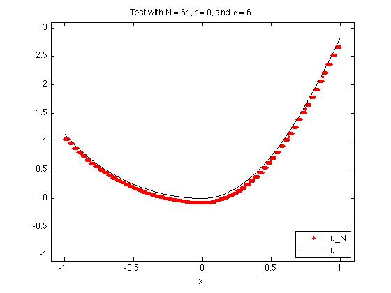
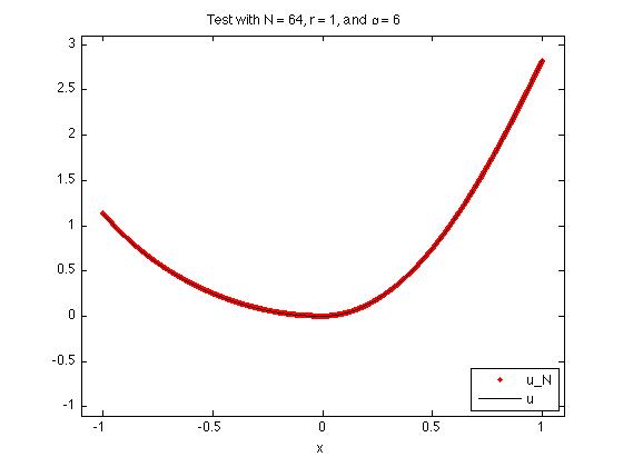
Refer to caption Refer to caption

r๐‘Ÿr Norm h=1/2โ„Ž12h=1/2 h=1/4โ„Ž14h=1/4 h=1/8โ„Ž18h=1/8 h=1/16โ„Ž116h=1/16 h=1/32โ„Ž132h=1/32 Error Error Order Error Order Error Order Error Order 0 L2superscript๐ฟ2L^{2} 1.8 9.0e-01 1.04 4.3e-01 1.05 2.1e-01 1.04 1.0e-01 1.02 Lโˆžsuperscript๐ฟL^{\infty} 2.5 1.2 0.99 6.2e-01 1.00 3.1e-01 1.00 1.6e-01 1.00 1 L2superscript๐ฟ2L^{2} 2.9e-01 6.3e-02 2.20 1.9e-02 1.73 7.0e-03 1.44 2.8e-03 1.34 Lโˆžsuperscript๐ฟL^{\infty} 2.9e-01 6.4e-02 2.17 2.0e-02 1.66 7.6e-03 1.42 3.1e-03 1.30 2 L2superscript๐ฟ2L^{2} 5.7e-03 8.2e-04 2.80 1.3e-04 2.66 3.2e-05 2.03 9.1e-06 1.81 Lโˆžsuperscript๐ฟL^{\infty} 2.0e-02 3.1e-03 2.70 4.2e-04 2.87 5.5e-05 2.94 8.0e-06 2.77 3 L2superscript๐ฟ2L^{2} 8.8e-04 7.7e-05 3.51 3.0e-06 4.68 1.4e-07 4.42 1.0e-08 3.76 Lโˆžsuperscript๐ฟL^{\infty} 2.1e-03 1.4e-04 3.90 8.6e-06 4.01 5.6e-07 3.94 9.5e-08 2.57

Fig. 2: Test 2 with ฮฑ=6๐›ผ6\alpha=6.

Test 3. Consider the stationary Hamilton-Jacobi-Bellman problem with finite dimensional control set

minฮธโ€‹(x)โˆˆ{1,2}โก{โˆ’ฮธโ€‹uxโ€‹x+uxโˆ’u+Sโ€‹(x)}subscript๐œƒ๐‘ฅ12๐œƒsubscript๐‘ข๐‘ฅ๐‘ฅsubscript๐‘ข๐‘ฅ๐‘ข๐‘†๐‘ฅ\displaystyle\min_{\theta(x)\in\{1,2\}}\left\{-\theta u_{xx}+u_{x}-u+S(x)\right\} =0,โˆ’1<x<1,formulae-sequenceabsent01๐‘ฅ1\displaystyle=0,\qquad-1<x<1,
uโ€‹(โˆ’1)=โˆ’1,uโ€‹(1)=1,formulae-sequence๐‘ข11๐‘ข11\displaystyle u(-1)=-1,\quad u(1)=1,

where

Sโ€‹(x)={โˆ’12โ€‹x2โˆ’4โ€‹|x|3+xโ€‹|x|3,x<024โ€‹x2โˆ’4โ€‹|x|3+xโ€‹|x|3,xโ‰ฅ0.๐‘†๐‘ฅcases12superscript๐‘ฅ24superscript๐‘ฅ3๐‘ฅsuperscript๐‘ฅ3๐‘ฅ024superscript๐‘ฅ24superscript๐‘ฅ3๐‘ฅsuperscript๐‘ฅ3๐‘ฅ0S(x)=\begin{cases}-12x^{2}-4|x|^{3}+x|x|^{3},&x<0\\ 24x^{2}-4|x|^{3}+x|x|^{3},&x\geq 0.\end{cases}

This problem has the exact solution uโ€‹(x)=xโ€‹|x|3๐‘ข๐‘ฅ๐‘ฅsuperscript๐‘ฅ3u(x)=x|x|^{3} corresponding to ฮธโˆ—โ€‹(x)=1superscript๐œƒ๐‘ฅ1\theta^{*}(x)=1 for x<0๐‘ฅ0x<0 and ฮธโˆ—โ€‹(x)=2superscript๐œƒ๐‘ฅ2\theta^{*}(x)=2 for xโ‰ฅ0๐‘ฅ0x\geq 0. Approximating the problem using various order elements, we have the following results recorded in Figureย 3. Again, due to the low regularity of the solution, we expect the rates of convergence to be affected. However, we still see increased accuracy for high order elements.
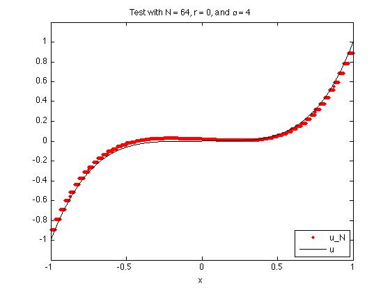
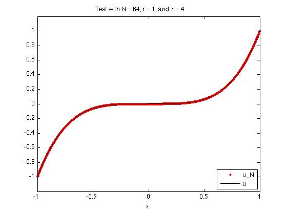
Refer to caption Refer to caption

r๐‘Ÿr Norm h=1/2โ„Ž12h=1/2 h=1/4โ„Ž14h=1/4 h=1/8โ„Ž18h=1/8 h=1/16โ„Ž116h=1/16 h=1/32โ„Ž132h=1/32 Error Error Order Error Order Error Order Error Order 0 L2superscript๐ฟ2L^{2} 5.0e-01 3.4e-01 0.53 1.3e-01 1.37 6.1e-02 1.12 4.4e-02 0.49 Lโˆžsuperscript๐ฟL^{\infty} 8.5e-01 5.7e-01 0.57 3.5e-01 0.72 2.0e-01 0.79 1.1e-01 0.86 1 L2superscript๐ฟ2L^{2} 1.4e-01 4.3e-02 1.72 9.7e-03 2.16 2.7e-03 1.85 7.3e-04 1.87 Lโˆžsuperscript๐ฟL^{\infty} 3.6e-01 1.1e-01 1.74 3.0e-02 1.87 7.8e-03 1.94 2.0e-03 1.97 2 L2superscript๐ฟ2L^{2} 2.8e-02 3.2e-03 3.10 4.0e-04 3.00 5.1e-05 2.99 6.4e-06 2.99 Lโˆžsuperscript๐ฟL^{\infty} 4.0e-02 5.5e-03 2.84 7.3e-04 2.93 9.3e-05 2.97 1.2e-05 2.98 3 L2superscript๐ฟ2L^{2} 9.4e-03 1.3e-03 2.91 1.6e-04 3.01 1.9e-05 3.01 2.4e-06 3.01 Lโˆžsuperscript๐ฟL^{\infty} 1.1e-02 1.5e-03 2.91 1.9e-04 3.02 2.3e-05 3.01 2.9e-06 3.01

Fig. 3: Test 3 with ฮฑ=4๐›ผ4\alpha=4.

Test 4. Consider the stationary Hamilton-Jacobi-Bellman problem with infinite dimensional control set

inf0<ฮธโ€‹(x)โ‰ค1{โˆ’ฮธโ€‹uxโ€‹x+ฮธ2โ€‹x2โ€‹ux+1xโ€‹u+Sโ€‹(x)}subscriptinfimum0๐œƒ๐‘ฅ1๐œƒsubscript๐‘ข๐‘ฅ๐‘ฅsuperscript๐œƒ2superscript๐‘ฅ2subscript๐‘ข๐‘ฅ1๐‘ฅ๐‘ข๐‘†๐‘ฅ\displaystyle\inf_{0<\theta(x)\leq 1}\left\{-\theta u_{xx}+\theta^{2}\,x^{2}\,u_{x}+\frac{1}{x}u+S(x)\right\} =0,absent0\displaystyle=0, 1.2<x<4,1.2๐‘ฅ4\displaystyle 1.2<x<4,
uโ€‹(1.2)=1.44โ€‹lnโก1.2,uโ€‹(4)=16โ€‹lnโก4,formulae-sequence๐‘ข1.21.441.2๐‘ข4164\displaystyle u(1.2)=1.44\ln 1.2,\quad u(4)=16\ln 4,

where

Sโ€‹(x)=4ln(x)2+12ln(x)+9โˆ’8x4ln(x)2โˆ’4x4ln(x)4โ€‹x3โ€‹[2โ€‹lnโก(x)+1].S(x)=\frac{4\ln(x)^{2}+12\ln(x)+9-8x^{4}\ln(x)^{2}-4x^{4}\ln(x)}{4x^{3}\left[2\ln(x)+1\right]}.

This problem has the exact solution uโ€‹(x)=x2โ€‹lnโกx๐‘ข๐‘ฅsuperscript๐‘ฅ2๐‘ฅu(x)=x^{2}\ln x corresponding to the control function ฮธโˆ—โ€‹(x)=2โ€‹lnโก(x)+32โ€‹x3โ€‹[2โ€‹lnโก(x)+1]superscript๐œƒ๐‘ฅ2๐‘ฅ32superscript๐‘ฅ3delimited-[]2๐‘ฅ1\theta^{*}(x)=\frac{2\ln(x)+3}{2x^{3}\left[2\ln(x)+1\right]}. Approximating the problem using various order elements, we obtain the results recorded in Figureย 4. We can see that the approximations appear to reach a maximal level of accuracy of about 5.0e-7 in both L2superscript๐ฟ2L^{2}- and Lโˆžsuperscript๐ฟL^{\infty}-norm, which is consistent with the results in Test 1 corresponding to r=2๐‘Ÿ2r=2.

Refer to caption Refer to caption

r๐‘Ÿr Norm h=2.8/4โ„Ž2.84h=2.8/4 h=2.8/8โ„Ž2.88h=2.8/8 h=2.8/16โ„Ž2.816h=2.8/16 h=2.8/32โ„Ž2.832h=2.8/32 h=2.8/64โ„Ž2.864h=2.8/64 Error Error Order Error Order Error Order Error Order 0 L2superscript๐ฟ2L^{2} 5.2 3.3 0.67 1.5 1.08 6.1e-01 1.34 2.6e-01 1.25 Lโˆžsuperscript๐ฟL^{\infty} 5.7 3.6 0.65 1.9 0.91 1.1 0.84 5.7e-01 0.91 1 L2superscript๐ฟ2L^{2} 2.6e-01 8.6e-02 1.60 2.6e-02 1.72 7.4e-03 1.83 2.0e-03 1.90 Lโˆžsuperscript๐ฟL^{\infty} 3.3e-01 1.1e-01 1.56 3.5e-02 1.67 1.1e-02 1.71 3.4e-03 1.65 2 L2superscript๐ฟ2L^{2} 2.6e-03 3.9e-04 2.77 6.6e-05 2.55 1.4e-05 2.26 3.2e-06 2.09 Lโˆžsuperscript๐ฟL^{\infty} 7.3e-03 1.0e-03 2.85 1.4e-04 2.91 1.9e-05 2.81 4.1e-06 2.25 3 L2superscript๐ฟ2L^{2} 6.4e-05 4.2e-06 3.93 3.1e-07 3.75 1.2e-07 1.35 1.2e-07 0.08 Lโˆžsuperscript๐ฟL^{\infty} 2.7e-04 2.1e-05 3.72 1.4e-06 3.84 8.7e-07 0.72 8.8e-07 -0.01

Fig. 4: Test 4 with ฮฑ=4๐›ผ4\alpha=4.

5.2 Parabolic test problems

We now implement the proposed fully discrete RK4 and trapezoidal LDG methods for approximating fully nonlinear parabolic equations of the form (2). While the above formulation makes no attempt to formally quantify a CFL condition for the RK4 method, for the tests we assume a CFL constraint of the form ฮ”โ€‹t=ฮบtโ€‹h2ฮ”๐‘กsubscript๐œ…๐‘กsuperscriptโ„Ž2\Delta t=\kappa_{t}h^{2}, and note that the constant ฮบtsubscript๐œ…๐‘ก\kappa_{t} appears to decrease as the order of the element increases. Below we implement both the RK4 method and the trapezoidal method for each test problem. However, we make no attempt to classify and compare the efficiency of the two methods. Instead, we focus on testing and demonstrating the usability of both fully discrete schemes and their promising potentials. For explicit scheme tests, we record the parameter ฮบtsubscript๐œ…๐‘ก\kappa_{t}, and for implicit scheme tests, we record the time step size ฮ”โ€‹tฮ”๐‘ก\Delta t. Note that the row 0โˆ—superscript00^{*} in the figures corresponding to the RK4 method refers to elements with r=0๐‘Ÿ0r=0 that use the standard L2superscript๐ฟ2L^{2} projection operator in (52).

Test 5. Let ฮฉ=(0,1)ฮฉ01\Omega=(0,1), uaโ€‹(t)=t4,ub=12+t4formulae-sequencesubscript๐‘ข๐‘Ž๐‘กsuperscript๐‘ก4subscript๐‘ข๐‘12superscript๐‘ก4u_{a}(t)=t^{4},u_{b}=\frac{1}{2}+t^{4}, and u0โ€‹(x)=12โ€‹x2subscript๐‘ข0๐‘ฅ12superscript๐‘ฅ2u_{0}(x)=\frac{1}{2}x^{2}. We consider the problem (2), (38), and (39) with

Fโ€‹(uxโ€‹x,ux,u,t,x)=โˆ’uxโ€‹xโ€‹u+12โ€‹x2+t4โˆ’4โ€‹t3+1.๐นsubscript๐‘ข๐‘ฅ๐‘ฅsubscript๐‘ข๐‘ฅ๐‘ข๐‘ก๐‘ฅsubscript๐‘ข๐‘ฅ๐‘ฅ๐‘ข12superscript๐‘ฅ2superscript๐‘ก44superscript๐‘ก31F(u_{xx},u_{x},u,t,x)=-u_{xx}\,u+\frac{1}{2}x^{2}+t^{4}-4\,t^{3}+1.

It is easy to verify that this problem has a unique classical solution uโ€‹(x,t)=0.5โ€‹x2+t4+1๐‘ข๐‘ฅ๐‘ก0.5superscript๐‘ฅ2superscript๐‘ก41u(x,t)=0.5\,x^{2}+t^{4}+1. Notice that the PDE has a product nonlinearity in the second order derivative. The numerical results for RK4 are presented in Figureย 5 and the results for the trapezoidal method are shown in Figureย 6. As expected, RK4 recovers the exact solution when r=2๐‘Ÿ2r=2.

Refer to caption ย ย ย ย ย  Refer to caption

r๐‘Ÿr Norm h=1/4โ„Ž14h=1/4 h=1/8โ„Ž18h=1/8 h=1/16โ„Ž116h=1/16 h=1/32โ„Ž132h=1/32 Error Error Order Error Order Error Order 0 L2superscript๐ฟ2L^{2} 9.9e-02 6.4e-02 0.64 3.6e-02 0.81 1.9e-02 0.92 Lโˆžsuperscript๐ฟL^{\infty} 2.2e-01 1.4e-01 0.64 8.0e-02 0.81 4.3e-02 0.89 1 L2superscript๐ฟ2L^{2} 5.7e-03 1.5e-03 1.98 3.7e-04 1.99 9.2e-05 1.99 Lโˆžsuperscript๐ฟL^{\infty} 8.0e-03 2.0e-03 1.99 5.1e-04 1.99 1.3e-04 1.99 2 L2superscript๐ฟ2L^{2} 2.4e-08 2.4e-08 0.00 2.4e-08 0.00 2.4e-08 -0.00 Lโˆžsuperscript๐ฟL^{\infty} 3.6e-08 3.7e-08 -0.03 3.7e-08 -0.01 3.7e-08 -0.01
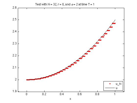
Fig. 5: Test 5: Computed solutions at T=1๐‘‡1T=1 using ฮบt=0.001subscript๐œ…๐‘ก0.001\kappa_{t}=0.001, ฮฑ=2๐›ผ2\alpha=2.

Refer to caption ย ย ย ย ย  Refer to caption

r๐‘Ÿr Norm h=1/4โ„Ž14h=1/4 h=1/8โ„Ž18h=1/8 h=1/16โ„Ž116h=1/16 h=1/32โ„Ž132h=1/32 Error Error Order Error Order Error Order 0 L2superscript๐ฟ2L^{2} 5.9e-02 3.4e-02 0.78 1.9e-02 0.84 1.0e-02 0.91 Lโˆžsuperscript๐ฟL^{\infty} 1.9e-01 1.1e-01 0.79 5.9e-02 0.90 3.0e-02 0.95 1 L2superscript๐ฟ2L^{2} 5.0e-03 1.4e-03 1.86 3.6e-04 1.94 9.1e-05 1.97 Lโˆžsuperscript๐ฟL^{\infty} 1.1e-02 2.8e-03 2.00 7.1e-04 2.00 1.8e-04 2.00 2 L2superscript๐ฟ2L^{2} 1.1e-07 1.1e-07 0.00 1.1e-07 0.00 1.1e-07 0.00 Lโˆžsuperscript๐ฟL^{\infty} 1.5e-07 1.6e-07 -0.04 1.6e-07 -0.01 1.6e-07 -0.00

Fig. 6: Test 5: Computed solution at T=1๐‘‡1T=1 using ฮ”โ€‹t=0.001ฮ”๐‘ก0.001\Delta t=0.001 and ฮฑ=2๐›ผ2\alpha=2.

Test 6. Let ฮฉ=(0,2)ฮฉ02\Omega=(0,2), uaโ€‹(t)=1subscript๐‘ข๐‘Ž๐‘ก1u_{a}(t)=1, ub=e2โ€‹(t+1)subscript๐‘ข๐‘superscript๐‘’2๐‘ก1u_{b}=e^{2(t+1)}, and u0โ€‹(x)=exsubscript๐‘ข0๐‘ฅsuperscript๐‘’๐‘ฅu_{0}(x)=e^{x}. We consider the problem (2), (38), and (39) with

Fโ€‹(uxโ€‹x,ux,u,t,x)=โˆ’uxโ€‹lnโก(uxโ€‹x+1)+Sโ€‹(x,t),๐นsubscript๐‘ข๐‘ฅ๐‘ฅsubscript๐‘ข๐‘ฅ๐‘ข๐‘ก๐‘ฅsubscript๐‘ข๐‘ฅsubscript๐‘ข๐‘ฅ๐‘ฅ1๐‘†๐‘ฅ๐‘กF(u_{xx},u_{x},u,t,x)=-u_{x}\ln\bigl{(}u_{xx}+1\bigr{)}+S(x,t),

and

Sโ€‹(x,t)=e(t+1)โ€‹xโ€‹(xโˆ’(t+1)โ€‹lnโก((t+1)2โ€‹e(t+1)โ€‹x+1)).๐‘†๐‘ฅ๐‘กsuperscript๐‘’๐‘ก1๐‘ฅ๐‘ฅ๐‘ก1superscript๐‘ก12superscript๐‘’๐‘ก1๐‘ฅ1S(x,t)=e^{(t+1)x}\Big{(}x-(t+1)\ln\bigl{(}(t+1)^{2}e^{(t+1)x}+1\bigr{)}\Big{)}.

It is easy to verify that this problem has a unique classical solution uโ€‹(x,t)=e(t+1)โ€‹x๐‘ข๐‘ฅ๐‘กsuperscript๐‘’๐‘ก1๐‘ฅu(x,t)=e^{(t+1)x}. Notice that this problem is nonlinear in both uxโ€‹xsubscript๐‘ข๐‘ฅ๐‘ฅu_{xx} and uxsubscript๐‘ข๐‘ฅu_{x}. Furthermore, the exact solution u๐‘ขu cannot be factored into the form uโ€‹(x,t)=Gโ€‹(t)โ€‹Yโ€‹(x)๐‘ข๐‘ฅ๐‘ก๐บ๐‘ก๐‘Œ๐‘ฅu(x,t)=G(t)\,Y(x) for some functions G๐บG and Y๐‘ŒY. Results for RK4 are given in Figureย 7, and results for the trapezoidal method are shown in Figureย 8. We note that RK4 was unstable without using the very restrictive values for ฮบtsubscript๐œ…๐‘ก\kappa_{t} recorded in Figureย 7. However, for RK4, we observe optimal rates of convergence in the spacial variable while the rates for the trapezoidal method appear to be limited by the lower rate of convergence for the time-stepping scheme.
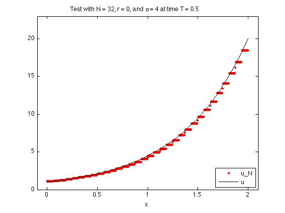
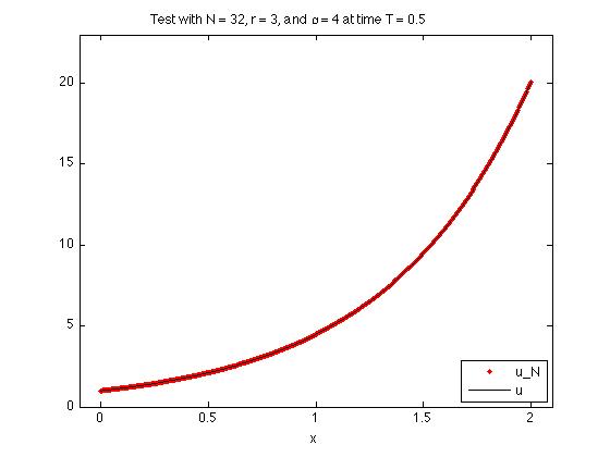
Refer to caption ย ย ย ย ย  Refer to caption

r๐‘Ÿr Norm h=2/4โ„Ž24h=2/4 h=2/8โ„Ž28h=2/8 h=2/16โ„Ž216h=2/16 h=2/32โ„Ž232h=2/32 Error Error Order Error Order Error Order 0 L2superscript๐ฟ2L^{2} 6.9e+00 5.7e+00 0.28 4.1e+00 0.47 2.6e+00 0.65 Lโˆžsuperscript๐ฟL^{\infty} 1.0e+01 7.9e+00 0.40 5.6e+00 0.50 3.7e+00 0.60 0โˆ—superscript00^{*} L2superscript๐ฟ2L^{2} 2.8e+00 1.5e+00 0.89 8.6e-01 0.82 5.1e-01 0.76 Lโˆžsuperscript๐ฟL^{\infty} 7.8e+00 5.0e+00 0.65 2.9e+00 0.76 1.6e+00 0.85 1 L2superscript๐ฟ2L^{2} 4.8e-01 1.2e-01 2.05 3.0e-02 1.93 8.2e-03 1.88 Lโˆžsuperscript๐ฟL^{\infty} 8.4e-01 2.3e-01 1.87 5.8e-02 1.99 1.5e-02 1.92 2 L2superscript๐ฟ2L^{2} 3.7e-02 7.8e-03 2.23 1.9e-03 2.03 4.8e-04 2.00 Lโˆžsuperscript๐ฟL^{\infty} 5.9e-02 1.0e-02 2.53 2.2e-03 2.19 5.2e-04 2.11 3 L2superscript๐ฟ2L^{2} 1.1e-03 7.4e-05 3.95 4.7e-06 3.99 3.01e-07 3.96 Lโˆžsuperscript๐ฟL^{\infty} 2.5e-03 1.6e-04 3.93 1.1e-05 3.86 7.66e-07 3.84

Fig. 7: Test 6: Computed solutions at time T=0.5๐‘‡0.5T=0.5 using ฮบt=0.005,0.001,0.0005,0.0001subscript๐œ…๐‘ก0.0050.0010.00050.0001\kappa_{t}=0.005,0.001,0.0005,0.0001 for r=0,1,2,3๐‘Ÿ0123r=0,1,2,3, respectively, and ฮฑ=4๐›ผ4\alpha=4. Left figure uses the standard L2superscript๐ฟ2L^{2} projection operator.

Refer to caption ย ย ย ย ย  Refer to caption

r๐‘Ÿr Norm h=2/4โ„Ž24h=2/4 h=2/8โ„Ž28h=2/8 h=2/16โ„Ž216h=2/16 h=2/32โ„Ž232h=2/32 Error Error Order Error Order Error Order 0 L2superscript๐ฟ2L^{2} 2.8e+00 1.5e+00 0.89 8.6e-01 0.82 5.1e-01 0.77 Lโˆžsuperscript๐ฟL^{\infty} 7.8e+00 5.0e+00 0.65 2.9e+00 0.76 1.6e+00 0.85 1 L2superscript๐ฟ2L^{2} 3.8e-01 1.3e-01 1.62 4.5e-02 1.49 1.5e-02 1.60 Lโˆžsuperscript๐ฟL^{\infty} 1.3e+00 4.0e-01 1.74 1.1e-01 1.85 3.0e-02 1.91 2 L2superscript๐ฟ2L^{2} 2.7e-02 6.7e-03 2.04 1.9e-03 1.82 5.3e-04 1.85 Lโˆžsuperscript๐ฟL^{\infty} 1.0e-01 1.5e-02 2.77 2.1e-03 2.80 5.4e-04 1.99 3 L2superscript๐ฟ2L^{2} 1.1e-03 7.2e-05 3.89 1.3e-05 2.46 1.2e-05 0.09 Lโˆžsuperscript๐ฟL^{\infty} 5.5e-03 4.0e-04 3.76 2.7e-05 3.92 1.3e-05 1.05

Fig. 8: Test 6: Computed solutions at time T=0.5๐‘‡0.5T=0.5 using ฮ”โ€‹t=0.005ฮ”๐‘ก0.005\Delta t=0.005 and ฮฑ=4๐›ผ4\alpha=4.

Test 7. Let ฮฉ=(0,2โ€‹ฯ€)ฮฉ02๐œ‹\Omega=(0,2\pi), uaโ€‹(t)=0subscript๐‘ข๐‘Ž๐‘ก0u_{a}(t)=0, ub=0subscript๐‘ข๐‘0u_{b}=0, and u0โ€‹(x)=sinโก(x)subscript๐‘ข0๐‘ฅ๐‘ฅu_{0}(x)=\sin(x). We consider the problem (2), (38), and (39) with

Fโ€‹(uxโ€‹x,ux,u,t,x)=โˆ’minฮธโ€‹(t,x)โˆˆ{1,2}โก{Aฮธโ€‹uxโ€‹xโˆ’cโ€‹(x,t)โ€‹cosโก(t)โ€‹sinโก(x)โˆ’sinโก(t)โ€‹sinโก(x)},๐นsubscript๐‘ข๐‘ฅ๐‘ฅsubscript๐‘ข๐‘ฅ๐‘ข๐‘ก๐‘ฅsubscript๐œƒ๐‘ก๐‘ฅ12subscript๐ด๐œƒsubscript๐‘ข๐‘ฅ๐‘ฅ๐‘๐‘ฅ๐‘ก๐‘ก๐‘ฅ๐‘ก๐‘ฅF(u_{xx},u_{x},u,t,x)=-\min_{\theta(t,x)\in\{1,2\}}\Big{\{}A_{\theta}\,u_{xx}-c(x,t)\cos(t)\,\sin(x)-\sin(t)\,\sin(x)\Big{\}},

where A1=1,A2=12formulae-sequencesubscript๐ด11subscript๐ด212A_{1}=1,A_{2}=\frac{1}{2}, and

cโ€‹(x,t)={1,ifย โ€‹0<tโ‰คฯ€2โ€‹ย andย โ€‹0<xโ‰คฯ€โ€‹ย orย โ€‹ฯ€2<tโ‰คฯ€โ€‹ย andย โ€‹ฯ€<x<2โ€‹ฯ€,12,otherwise.๐‘๐‘ฅ๐‘กcases1ifย 0๐‘ก๐œ‹2ย andย 0๐‘ฅ๐œ‹ย orย ๐œ‹2๐‘ก๐œ‹ย andย ๐œ‹๐‘ฅ2๐œ‹12otherwisec(x,t)=\begin{cases}1,&\text{if }0<t\leq\frac{\pi}{2}\mbox{ and }0<x\leq\pi\text{ or }\frac{\pi}{2}<t\leq\pi\text{ and }\pi<x<2\pi,\\ \frac{1}{2},&\mbox{otherwise}.\end{cases}

It is easy to check that this problem has a unique classical solution uโ€‹(x,t)=cosโก(t)โ€‹sinโก(x)๐‘ข๐‘ฅ๐‘ก๐‘ก๐‘ฅu(x,t)=\cos(t)\sin(x). Notice that this problem has a finite dimensional control parameter set, and the optimal control is given by

ฮธโˆ—โ€‹(t,x)={1,ifย โ€‹cโ€‹(x,t)=1,2,ifย โ€‹cโ€‹(x,t)=12.superscript๐œƒ๐‘ก๐‘ฅcases1ifย ๐‘๐‘ฅ๐‘ก12ifย ๐‘๐‘ฅ๐‘ก12\theta^{*}(t,x)=\begin{cases}1,&\mbox{if }c(x,t)=1,\\ 2,&\mbox{if }c(x,t)=\frac{1}{2}.\end{cases}

The numerical results are reported in Figureย 9 for RK4 and in Figureย 10 for the trapezoidal method.

Refer to caption ย ย ย ย ย  Refer to caption

r๐‘Ÿr Norm h=ฯ€/2โ„Ž๐œ‹2h=\pi/2 h=ฯ€/4โ„Ž๐œ‹4h=\pi/4 h=ฯ€/8โ„Ž๐œ‹8h=\pi/8 h=ฯ€/16โ„Ž๐œ‹16h=\pi/16 Error Error Order Error Order Error Order 0 L2superscript๐ฟ2L^{2} 1.5e+00 1.3e+00 0.24 7.1e-01 0.82 3.3e-01 1.12 Lโˆžsuperscript๐ฟL^{\infty} 9.6e-01 7.7e-01 0.31 4.9e-01 0.65 2.9e-01 0.78 0โˆ—superscript00^{*} L2superscript๐ฟ2L^{2} 1.2e+00 6.9e-01 0.78 3.0e-01 1.19 1.4e-01 1.16 Lโˆžsuperscript๐ฟL^{\infty} 9.2e-01 5.8e-01 0.67 3.2e-01 0.85 1.8e-01 0.83 1 L2superscript๐ฟ2L^{2} 2.7e-01 7.6e-02 1.81 2.0e-02 1.94 5.0e-03 1.99 Lโˆžsuperscript๐ฟL^{\infty} 1.9e-01 6.6e-02 1.52 1.7e-02 1.97 4.2e-03 2.00 2 L2superscript๐ฟ2L^{2} 7.2e-02 1.8e-02 1.98 4.5e-03 2.02 1.1e-03 2.01 Lโˆžsuperscript๐ฟL^{\infty} 6.8e-02 1.8e-02 1.93 4.3e-03 2.04 1.1e-03 2.03 3 L2superscript๐ฟ2L^{2} 8.3e-03 5.7e-04 3.87 3.6e-05 3.97 2.2e-06 4.02 Lโˆžsuperscript๐ฟL^{\infty} 7.6e-03 5.1e-04 3.92 3.2e-05 4.00 1.9e-06 4.04
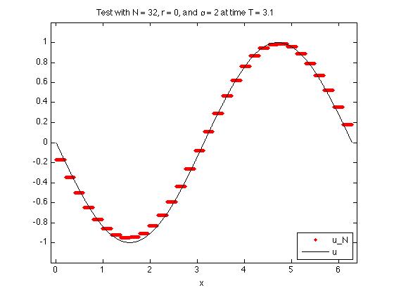
Fig. 9: Test 7: Computed solutions at time T=3.10๐‘‡3.10T=3.10 using ฮบt=0.05,0.005,0.001,0.0005subscript๐œ…๐‘ก0.050.0050.0010.0005\kappa_{t}=0.05,0.005,0.001,0.0005 for r=0,1,2,3๐‘Ÿ0123r=0,1,2,3, respectively, and ฮฑ=2๐›ผ2\alpha=2. Left plot uses the standard L2superscript๐ฟ2L^{2} projection operator.

Refer to caption ย ย ย ย ย  Refer to caption

r๐‘Ÿr Norm h=ฯ€/2โ„Ž๐œ‹2h=\pi/2 h=ฯ€/4โ„Ž๐œ‹4h=\pi/4 h=ฯ€/8โ„Ž๐œ‹8h=\pi/8 h=ฯ€/16โ„Ž๐œ‹16h=\pi/16 Error Error Order Error Order Error Order 0 L2superscript๐ฟ2L^{2} 1.2e+00 6.9e-01 0.78 3.0e-01 1.19 1.4e-01 1.16 Lโˆžsuperscript๐ฟL^{\infty} 9.2e-01 5.8e-01 0.67 3.2e-01 0.85 1.8e-01 0.83 1 L2superscript๐ฟ2L^{2} 2.3e-01 7.5e-02 1.63 2.0e-02 1.89 7.9e-03 1.36 Lโˆžsuperscript๐ฟL^{\infty} 2.1e-01 6.6e-02 1.66 1.7e-02 1.95 5.8e-03 1.56 2 L2superscript๐ฟ2L^{2} 6.9e-02 1.8e-02 1.93 4.7e-03 1.95 2.5e-03 0.90 Lโˆžsuperscript๐ฟL^{\infty} 6.5e-02 1.8e-02 1.87 4.5e-03 2.00 1.9e-03 1.21 3 L2superscript๐ฟ2L^{2} 8.1e-03 5.9e-04 3.79 1.1e-04 2.42 1.1e-04 0.03 Lโˆžsuperscript๐ฟL^{\infty} 7.5e-03 5.2e-04 3.87 7.6e-05 2.77 7.3e-05 0.06

Fig. 10: Test 7: Computed solutions at time T=3.10๐‘‡3.10T=3.10 using ฮ”โ€‹t=0.031ฮ”๐‘ก0.031\Delta t=0.031 and ฮฑ=2๐›ผ2\alpha=2.

Test 8. Let ฮฉ=(0,3)ฮฉ03\Omega=(0,3), uaโ€‹(t)=eโˆ’tsubscript๐‘ข๐‘Ž๐‘กsuperscript๐‘’๐‘กu_{a}(t)=e^{-t}, ub=8โ€‹eโˆ’tsubscript๐‘ข๐‘8superscript๐‘’๐‘กu_{b}=8\,e^{-t}, and u0โ€‹(x)=|xโˆ’1|3subscript๐‘ข0๐‘ฅsuperscript๐‘ฅ13u_{0}(x)=|x-1|^{3}. We consider the problem (2), (38), and (39) with

Fโ€‹(uxโ€‹x,ux,u,t,x)=โˆ’infโˆ’1โ‰คฮธโ€‹(t,x)โ‰ค1{|xโˆ’1|โ€‹uxโ€‹x+ฮธโ€‹ux}โˆ’|xโˆ’1|2โ€‹(|xโˆ’1|โˆ’3)โ€‹eโˆ’t,๐นsubscript๐‘ข๐‘ฅ๐‘ฅsubscript๐‘ข๐‘ฅ๐‘ข๐‘ก๐‘ฅsubscriptinfimum1๐œƒ๐‘ก๐‘ฅ1๐‘ฅ1subscript๐‘ข๐‘ฅ๐‘ฅ๐œƒsubscript๐‘ข๐‘ฅsuperscript๐‘ฅ12๐‘ฅ13superscript๐‘’๐‘กF(u_{xx},u_{x},u,t,x)=-\inf_{-1\leq\theta(t,x)\leq 1}\Big{\{}|x-1|u_{xx}+\theta u_{x}\Big{\}}-|x-1|^{2}\,\left(|x-1|-3\right)\,e^{-t},

It is easy to verify that the problem has the exact solution uโ€‹(t,x)=|xโˆ’1|3โ€‹eโˆ’t๐‘ข๐‘ก๐‘ฅsuperscript๐‘ฅ13superscript๐‘’๐‘กu(t,x)=|x-1|^{3}\,e^{-t}. Notice that the above operator is not elliptic for x=1๐‘ฅ1x=1. Also, this problem has a bang-bang type control with the optimal control given by

ฮธโˆ—โ€‹(t,x)={1,ifย โ€‹x<1,โˆ’1,ifย โ€‹x>1.superscript๐œƒ๐‘ก๐‘ฅcases1ifย ๐‘ฅ11ifย ๐‘ฅ1\theta^{*}(t,x)=\begin{cases}1,&\text{if }x<1,\\ -1,&\text{if }x>1.\end{cases}

We can see from the results for the RK4 method in Figureย 11 and the results for the trapezoidal method in Figureย 12 that the spatial rates of convergence appear to be limited by the low regularity of the solution, while the accuracy appears to increase with respect to the element degree.
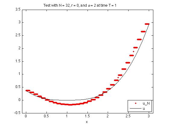
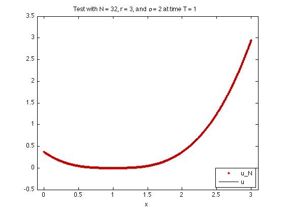
Refer to caption ย ย ย ย ย  Refer to caption

r๐‘Ÿr Norm h=3/4โ„Ž34h=3/4 h=3/8โ„Ž38h=3/8 h=3/16โ„Ž316h=3/16 h=3/32โ„Ž332h=3/32 Error Error Order Error Order Error Order 0 L2superscript๐ฟ2L^{2} 2.1e+00 1.4e+00 0.51 5.3e-01 1.44 2.9e-01 0.88 Lโˆžsuperscript๐ฟL^{\infty} 2.1e+00 1.5e+00 0.44 8.5e-01 0.86 4.9e-01 0.81 0โˆ—superscript00^{*} L2superscript๐ฟ2L^{2} 8.6e-01 8.8e-01 -0.02 5.9e-01 0.58 2.9e-01 1.00 Lโˆžsuperscript๐ฟL^{\infty} 1.8e+00 1.3e+00 0.53 7.3e-01 0.80 3.9e-01 0.92 1 L2superscript๐ฟ2L^{2} 2.0e-01 7.3e-02 1.45 1.3e-02 2.44 3.2e-03 2.06 Lโˆžsuperscript๐ฟL^{\infty} 3.9e-01 1.0e-01 1.92 2.7e-02 1.95 6.8e-03 1.98 2 L2superscript๐ฟ2L^{2} 1.1e-01 2.0e-02 2.49 5.2e-03 1.98 1.3e-03 2.02 Lโˆžsuperscript๐ฟL^{\infty} 1.1e-01 2.0e-02 2.42 5.2e-03 1.99 1.3e-03 2.00 3 L2superscript๐ฟ2L^{2} 3.0e-02 6.8e-03 2.13 1.7e-03 2.00 4.2e-04 2.03 Lโˆžsuperscript๐ฟL^{\infty} 2.9e-02 6.9e-03 2.08 1.7e-03 2.02 4.2e-04 2.02
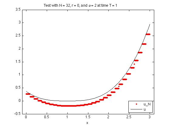
Fig. 11: Test 8: Computed solutions at time T=1๐‘‡1T=1 using ฮบt=0.05,0.005,0.001,0.0005subscript๐œ…๐‘ก0.050.0050.0010.0005\kappa_{t}=0.05,0.005,0.001,0.0005 for r=0,1,2,3๐‘Ÿ0123r=0,1,2,3, respectively, and ฮฑ=2๐›ผ2\alpha=2.

Refer to caption ย ย ย ย ย  Refer to caption

r๐‘Ÿr Norm h=3/4โ„Ž34h=3/4 h=3/8โ„Ž38h=3/8 h=3/16โ„Ž316h=3/16 h=3/32โ„Ž332h=3/32 Error Error Order Error Order Error Order 0 L2superscript๐ฟ2L^{2} 8.6e-01 8.8e-01 -0.02 5.9e-01 0.58 2.9e-01 1.00 Lโˆžsuperscript๐ฟL^{\infty} 1.8e+00 1.3e+00 0.53 7.3e-01 0.80 3.9e-01 0.92 1 L2superscript๐ฟ2L^{2} 2.0e-01 7.3e-02 1.45 1.3e-02 2.44 3.2e-03 2.05 Lโˆžsuperscript๐ฟL^{\infty} 3.9e-01 1.0e-01 1.92 2.7e-02 1.95 6.8e-03 1.98 2 L2superscript๐ฟ2L^{2} 1.1e-01 2.0e-02 2.49 5.2e-03 1.98 1.3e-03 2.02 Lโˆžsuperscript๐ฟL^{\infty} 1.1e-01 2.0e-02 2.42 5.2e-03 1.99 1.3e-03 2.00 3 L2superscript๐ฟ2L^{2} 3.0e-02 6.8e-03 2.13 1.7e-03 2.00 4.2e-04 2.03 Lโˆžsuperscript๐ฟL^{\infty} 2.9e-02 6.9e-03 2.08 1.7e-03 2.02 4.2e-04 2.02

Fig. 12: Test 8: Computed solutions at time T=1๐‘‡1T=1 using ฮ”โ€‹t=0.001ฮ”๐‘ก0.001\Delta t=0.001 and ฮฑ=2๐›ผ2\alpha=2.

5.3 The role of the numerical moment

In this section, we focus on understanding the role of the numerical moment. We first give an interpretation of the numerical moment, and then we explore the utility of the numerical moment. The role of the numerical moment can heuristically be understood as follows when the numerical moment is rewritten in the form

h2โ€‹ฮฑโ€‹(p1โ€‹hโˆ’p2โ€‹hโˆ’p3โ€‹h+p4โ€‹hh2).superscriptโ„Ž2๐›ผsubscript๐‘1โ„Žsubscript๐‘2โ„Žsubscript๐‘3โ„Žsubscript๐‘4โ„Žsuperscriptโ„Ž2h^{2}\,\alpha\,\Bigl{(}\frac{p_{1h}-p_{2h}-p_{3h}+p_{4h}}{h^{2}}\Bigr{)}.

Letting r=0๐‘Ÿ0r=0, we see that p1โ€‹hโˆ’p2โ€‹hโˆ’p3โ€‹h+p4โ€‹hh2subscript๐‘1โ„Žsubscript๐‘2โ„Žsubscript๐‘3โ„Žsubscript๐‘4โ„Žsuperscriptโ„Ž2\frac{p_{1h}-p_{2h}-p_{3h}+p_{4h}}{h^{2}} is an ๐’ชโ€‹(h2)๐’ชsuperscriptโ„Ž2\mathcal{O}(h^{2}) approximation to uxโ€‹xโ€‹xโ€‹xsubscript๐‘ข๐‘ฅ๐‘ฅ๐‘ฅ๐‘ฅu_{xxxx}. Then, we can see that the numerical moment acts as a centered difference approximation for ฮ”2โ€‹usuperscriptฮ”2๐‘ข\Delta^{2}u multiplied by a factor that tends to zero with rate ๐’ชโ€‹(h2)๐’ชsuperscriptโ„Ž2\mathcal{O}(h^{2}). Thus, at the PDE level, we are in essence approximating the fully nonlinear second order elliptic operator

Fโ€‹(uxโ€‹x,ux,u,x)๐นsubscript๐‘ข๐‘ฅ๐‘ฅsubscript๐‘ข๐‘ฅ๐‘ข๐‘ฅF\left(u_{xx},u_{x},u,x\right)

by the quasilinear fourth order operator F~ฯsubscript~๐น๐œŒ\widetilde{F}_{\rho}, where

F~ฯโ€‹(uxโ€‹xโ€‹xโ€‹x,uxโ€‹x,ux,u,x)=ฯโ€‹uxโ€‹xโ€‹xโ€‹x+Fโ€‹(uxโ€‹x,ux,u,x).subscript~๐น๐œŒsubscript๐‘ข๐‘ฅ๐‘ฅ๐‘ฅ๐‘ฅsubscript๐‘ข๐‘ฅ๐‘ฅsubscript๐‘ข๐‘ฅ๐‘ข๐‘ฅ๐œŒsubscript๐‘ข๐‘ฅ๐‘ฅ๐‘ฅ๐‘ฅ๐นsubscript๐‘ข๐‘ฅ๐‘ฅsubscript๐‘ข๐‘ฅ๐‘ข๐‘ฅ\widetilde{F}_{\rho}\left(u_{xxxx},u_{xx},u_{x},u,x\right)=\rho\,u_{xxxx}+F\left(u_{xx},u_{x},u,x\right).

In the limit as ฯโ†’0โ†’๐œŒ0\rho\to 0, we heuristically expect that the solution of the fourth order problem converges to the unique viscosity solution of the second order problem. Using a convergent family of fourth order quasilinear PDEs to approximate a fully nonlinear second order PDE has previously been considered for PDEs such as the Monge-Ampรจre equation, the prescribed Gauss curvature equation, the infinity-Laplace equation, and linear second order equations of non-divergence form. The method is known as the vanishing moment method. We refer the reader to [13, 8] for a detailed exposition.

We now show that the proposed schemes using a numerical moment can eliminate the numerical artifacts that arise as consequences from using a standard discretization, and in certain cases when the numerical artifacts are not fully eliminated, the algebraic system has enough structure to design solvers that emphasize the monotonicity in p2+p32subscript๐‘2subscript๐‘32\frac{p_{2}+p_{3}}{2} and are consistent in searching for solutions at which the nonlinear PDE problem is elliptic. We again consider the Monge-Ampรจre type problem from Test 1 in sectionย 5.1. The given problem has two classical PDE solutions u+superscript๐‘ขu^{+} and uโˆ’superscript๐‘ขu^{-}. However, there exists infinitely many C1superscript๐ถ1C^{1} functions that satisfy the PDE and boundary conditions almost everywhere, as seen by ฮผ๐œ‡\mu in (62). These almost everywhere solutions will correspond to what we call numerical artifacts in that algebraic solutions for a given discretization may correspond to these functions. It is well known that using a standard discretization scheme for the Monge-Ampรจre problem can yield multiple solutions, many of which are numerical artifacts that do not correspond to PDE solutions [8]. For example, let ฮผโˆˆH2โ€‹(0,1)โˆ–C2โ€‹(0,1)๐œ‡superscript๐ป201superscript๐ถ201\mu\in H^{2}(0,1)\setminus C^{2}(0,1) be defined by

(62) ฮผโ€‹(x)={12โ€‹x2+14โ€‹x,forย โ€‹x<0.5,โˆ’12โ€‹x2+54โ€‹xโˆ’14,forย โ€‹xโ‰ฅ0.5.๐œ‡๐‘ฅcases12superscript๐‘ฅ214๐‘ฅforย ๐‘ฅ0.512superscript๐‘ฅ254๐‘ฅ14forย ๐‘ฅ0.5\mu(x)=\begin{cases}\frac{1}{2}x^{2}+\frac{1}{4}x,&\text{for }x<0.5,\\ -\frac{1}{2}x^{2}+\frac{5}{4}x-\frac{1}{4},&\text{for }x\geq 0.5.\end{cases}

Furthermore, suppose xj=0.5subscript๐‘ฅ๐‘—0.5x_{j}=0.5 for some j=2,3,โ€ฆ,Jโˆ’1๐‘—23โ€ฆ๐ฝ1j=2,3,\ldots,J-1. Then, when using a standard central difference discretization, ฮผ๐œ‡\mu corresponds to a numerical solution, yielding a numerical artifact.

We now consider our discretization that uses a numerical moment. When ฮฑ=0๐›ผ0\alpha=0, we have no numerical moment. As a result, we have numerical artifacts as in the standard central difference discretization case. Suppose r=0๐‘Ÿ0r=0. Then, for ฮฑโ‰ 0๐›ผ0\alpha\neq 0, inspection of (27)โ€“(30) yields the fact that p2โ€‹hsubscript๐‘2โ„Žp_{2h} cannot jump from a value of 111 to a value of โˆ’11-1 when going across xj=0.5subscript๐‘ฅ๐‘—0.5x_{j}=0.5. Thus, the numerical moment penalizes discontinuities in pjโ€‹hsubscript๐‘๐‘—โ„Žp_{jh}, j=1,2,3,4๐‘—1234j=1,2,3,4, and, as a result, the numerical moment eliminates numerical artifacts such as ฮผ๐œ‡\mu. Similarly, for r=1๐‘Ÿ1r=1, we can see that ฮผ๐œ‡\mu does not correspond to a numerical solution. However, in this case, the algebraic system does have a small residual that may trap solvers such as fsolve. Thus, for r=0๐‘Ÿ0r=0 and r=1๐‘Ÿ1r=1, the numerical moment penalizes differences in pjโ€‹hsubscript๐‘๐‘—โ„Žp_{jh}, j=1,2,3,4๐‘—1234j=1,2,3,4, that arise from discontinuities in uhsubscript๐‘ขโ„Žu_{h}, q1โ€‹hsubscript๐‘ž1โ„Žq_{1h}, and q2โ€‹hsubscript๐‘ž2โ„Žq_{2h}. Hence, it eliminates numerical artifacts such as ฮผ๐œ‡\mu.

We now consider rโ‰ฅ2๐‘Ÿ2r\geq 2, in which case ฮผโˆˆVh๐œ‡superscript๐‘‰โ„Ž\mu\in V^{h}. Furthermore, since ฮผโˆˆC1๐œ‡superscript๐ถ1\mu\in C^{1}, we will end up with uh=ฮผsubscript๐‘ขโ„Ž๐œ‡u_{h}=\mu, q1โ€‹h=q2โ€‹hsubscript๐‘ž1โ„Žsubscript๐‘ž2โ„Žq_{1h}=q_{2h}, and p1โ€‹h=pjโ€‹hsubscript๐‘1โ„Žsubscript๐‘๐‘—โ„Žp_{1h}=p_{jh} for j=2,3,4๐‘—234j=2,3,4 being a numeric solution, where

q1โ€‹hโ€‹(x)={x+14,forย โ€‹x<0.5,โˆ’x+54,forย โ€‹x>0.5,andp1โ€‹hโ€‹(x)={1,forย โ€‹x<0.5,โˆ’1,forย โ€‹x>0.5.formulae-sequencesubscript๐‘ž1โ„Ž๐‘ฅcases๐‘ฅ14forย ๐‘ฅ0.5๐‘ฅ54forย ๐‘ฅ0.5andsubscript๐‘1โ„Ž๐‘ฅcases1forย ๐‘ฅ0.51forย ๐‘ฅ0.5q_{1h}(x)=\begin{cases}x+\frac{1}{4},&\text{for }x<0.5,\\ -x+\frac{5}{4},&\text{for }x>0.5,\end{cases}\qquad\text{and}\qquad p_{1h}(x)=\begin{cases}1,&\text{for }x<0.5,\\ -1,&\text{for }x>0.5.\end{cases}

Thus, by the equalities of pjโ€‹hsubscript๐‘๐‘—โ„Žp_{jh}, j=1,2,3,4๐‘—1234j=1,2,3,4, the numerical moment is always zero and we do have numerical artifacts. These equalities are a consequence of the continuity of uhsubscript๐‘ขโ„Žu_{h}, q1โ€‹hsubscript๐‘ž1โ„Žq_{1h}, and q2โ€‹hsubscript๐‘ž2โ„Žq_{2h}. With the extra degrees of freedom for rโ‰ฅ2๐‘Ÿ2r\geq 2, we allow C1superscript๐ถ1C^{1} to be embedded into our approximation space Vhsuperscript๐‘‰โ„ŽV^{h}, thus creating possible solutions with a zero valued numerical moment. The numerical moment acts as a penalty term for differences in pjโ€‹hsubscript๐‘๐‘—โ„Žp_{jh}, j=1,2,3,4๐‘—1234j=1,2,3,4, which are a consequence of discontinuities in q1โ€‹hsubscript๐‘ž1โ„Žq_{1h} and q2โ€‹hsubscript๐‘ž2โ„Žq_{2h} that naturally arise for nontrivial functions when r=0๐‘Ÿ0r=0 or r=1๐‘Ÿ1r=1.

Even with the possible presence of numerical artifacts for the above discretization when rโ‰ฅ2๐‘Ÿ2r\geq 2, the numerical moment can be exploited at the solver level. We now present a splitting algorithm for solving the resulting nonlinear algebraic system that uses the numerical moment to strongly emphasize the fact that the viscosity solution of the PDE should preserve the monotonicity required by the definition of ellipticity.

Algorithm 5.1.
  1. (1)

    Pick an initial guess for uhsubscript๐‘ขโ„Žu_{h}.

  2. (2)

    Form initial guesses for q1โ€‹hsubscript๐‘ž1โ„Žq_{1h}, q2โ€‹hsubscript๐‘ž2โ„Žq_{2h}, p1โ€‹hsubscript๐‘1โ„Žp_{1h}, p2โ€‹hsubscript๐‘2โ„Žp_{2h}, p3โ€‹hsubscript๐‘3โ„Žp_{3h}, and p4โ€‹hsubscript๐‘4โ„Žp_{4h} using equations (35) and (36).

  3. (3)

    Solve equation (20) for p2โ€‹h+p3โ€‹h2subscript๐‘2โ„Žsubscript๐‘3โ„Ž2\frac{p_{2h}+p_{3h}}{2}.

  4. (4)

    Solve equation (35) for i=1,2๐‘–12i=1,2 and the equation formed by averaging (36) for j=2,3๐‘—23j=2,3 for uhsubscript๐‘ขโ„Žu_{h}, q1โ€‹hsubscript๐‘ž1โ„Žq_{1h}, and q2โ€‹hsubscript๐‘ž2โ„Žq_{2h}.

  5. (5)

    Solve equation (36) for j=1,2,3,4๐‘—1234j=1,2,3,4 for p1โ€‹hsubscript๐‘1โ„Žp_{1h}, p2โ€‹hsubscript๐‘2โ„Žp_{2h}, p3โ€‹hsubscript๐‘3โ„Žp_{3h}, and p4โ€‹hsubscript๐‘4โ„Žp_{4h}.

  6. (6)

    Repeat Steps 3 - 5 until the change in p2โ€‹h+p3โ€‹h2subscript๐‘2โ„Žsubscript๐‘3โ„Ž2\frac{p_{2h}+p_{3h}}{2} is sufficiently small.

For the next numerical tests, we will show that using Algorithmย 5.1 with a sufficiently large coefficient for the numerical moment destabilizes numerical artifacts such as ฮผ๐œ‡\mu and steers the approximation towards the viscosity solution of the PDE. Let uยฏโ€‹(x)=x2ยฏ๐‘ข๐‘ฅ๐‘ฅ2\overline{u}(x)=\frac{x}{2}. Then, uยฏยฏ๐‘ข\overline{u} is the secant line formed by the boundary data for the given boundary value problem. We now approximate the solution of the Monge-Ampรจre type problem from Test 1 in sectionย 5.1 by using 100 iterations of Algorithmย 5.1 followed by using fsolve on the full system to solve the global discretization given by (20), (35), and (36). We take the initial guess to be

uh(0)=34โ€‹ฮผ+14โ€‹uยฏ,superscriptsubscript๐‘ขโ„Ž034๐œ‡14ยฏ๐‘ขu_{h}^{(0)}=\frac{3}{4}\mu+\frac{1}{4}\overline{u},

where, for r=0๐‘Ÿ0r=0, uh0superscriptsubscript๐‘ขโ„Ž0u_{h}^{0} is first projected into Vhsuperscript๐‘‰โ„ŽV^{h}. From Figureย 13, we see that the numerical moment drives the solution towards the viscosity solution u+superscript๐‘ขu^{+} when r=0๐‘Ÿ0r=0 and ฮฑ๐›ผ\alpha is positive. From Figureย 14, we see that the numerical moment also drives the solution towards the viscosity solution u+superscript๐‘ขu^{+} when r=2๐‘Ÿ2r=2 and ฮฑ๐›ผ\alpha is positive, despite the presence of numerical artifacts. From Figureย 15, we see that the moment drives the solution towards the viscosity solution of Fโ€‹(uxโ€‹x,ux,u,x):=uxโ€‹x2โˆ’1assign๐นsubscript๐‘ข๐‘ฅ๐‘ฅsubscript๐‘ข๐‘ฅ๐‘ข๐‘ฅsuperscriptsubscript๐‘ข๐‘ฅ๐‘ฅ21F(u_{xx},u_{x},u,x):=u_{xx}^{2}-1 given by uโˆ’superscript๐‘ขu^{-} for r=0๐‘Ÿ0r=0 and r=2๐‘Ÿ2r=2 when ฮฑ๐›ผ\alpha is chosen to be negative. In each figure, the middle graph corresponds to ฮผ๐œ‡\mu. Clearly, we recover the numerical artifact corresponding to ฮผ๐œ‡\mu when ฮฑ=0๐›ผ0\alpha=0. Thus, the numerical moment plays an essential role in either eliminating numerical artifacts at the discretization level or handling numerical artifacts at the solver level.

We make one final note about using the iterative solver given by Algorithmย 5.1. Note that using fsolve to solve the full system with the initial guess given by uh(0)superscriptsubscript๐‘ขโ„Ž0u_{h}^{(0)} resulted in either not finding a root for many tests (r=1๐‘Ÿ1r=1) or converging to a numerical artifact with a discontinuous second order derivative at another node in the mesh (r=2๐‘Ÿ2r=2). In order to use fsolve for the given test problem, the initial guess should either be restricted to the class of functions where p2โ€‹hsubscript๐‘2โ„Žp_{2h} and p3โ€‹hsubscript๐‘3โ„Žp_{3h} preserve the ellipticity of the nonlinear operator, the initial guess should be preconditioned by first using fsolve with r=0,1๐‘Ÿ01r=0,1, or the initial guess should be preconditioned using Algorithmย 5.1. When using r=0๐‘Ÿ0r=0 and a non-ellipticity-preserving initial guess, solving the full system of equations with fsolve still has the potential to converge to uโˆ’superscript๐‘ขu^{-} even for ฮฑ>0๐›ผ0\alpha>0. The strength of Algorithmย 5.1 is that it strongly enforces the requirement that F^^๐น\widehat{F} is monotone decreasing in p2subscript๐‘2p_{2} and p3subscript๐‘3p_{3} over each iteration. Thus, a sufficiently large value for ฮฑ๐›ผ\alpha drives the approximation towards the class of ellipticity-preserving functions if the algorithm converges.
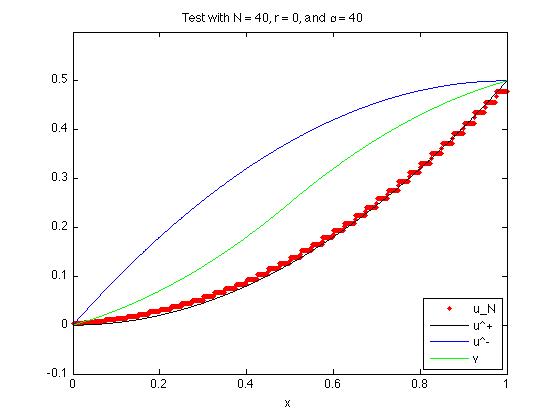
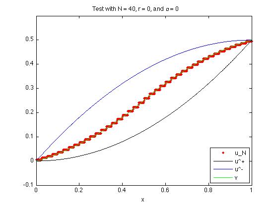
Refer to caption ย ย ย ย ย  Refer to caption

Fig. 13: Left: ฮฑ=40๐›ผ40\alpha=40, h=1/40โ„Ž140h=1/40, and r=0๐‘Ÿ0r=0. Right: ฮฑ=0๐›ผ0\alpha=0, h=1/40โ„Ž140h=1/40, and r=0๐‘Ÿ0r=0

Refer to caption ย ย ย ย ย  Refer to caption

Fig. 14: Left: ฮฑ=20๐›ผ20\alpha=20, h=1/20โ„Ž120h=1/20, and r=2๐‘Ÿ2r=2. Right: ฮฑ=0๐›ผ0\alpha=0, h=1/20โ„Ž120h=1/20, and r=2๐‘Ÿ2r=2

Refer to caption ย ย ย ย ย  Refer to caption

Fig. 15: Left: ฮฑ=โˆ’40๐›ผ40\alpha=-40, h=1/40โ„Ž140h=1/40, and r=0๐‘Ÿ0r=0. Right: ฮฑ=โˆ’20๐›ผ20\alpha=-20, h=1/20โ„Ž120h=1/20, and r=2๐‘Ÿ2r=2

References

  • [1] M.ย Bardi and I.ย Capuzzo-Dolcetta. Optimal control and viscosity solutions of Hamilton-Jacobi-Bellman equations, Systems & Control: Foundations & Applications. Birkhรคuser Boston Inc., Boston, MA, 1997.
  • [2] G.ย Barles and P.ย E. Souganidis. Convergence of approximation schemes for fully nonlinear second order equations. Asymptotic Anal., 4ย (3):271โ€“283, 1991.
  • [3] L.ย A. Caffarelli and X.ย Cabrรฉ. Fully nonlinear elliptic equations, Vol.ย 43 of American Mathematical Society Colloquium Publications. American Mathematical Society, Providence, RI, 1995.
  • [4] L.ย A. Caffarelli and P.ย A. Souganidis. A rate of convergence for monotone finite difference approximations to fully nonlinear, uniformly elliptic PDEs. Comm. Pure Appl. Math., 61:1โ€“17, 2008.
  • [5] M.ย G. Crandall and P.-L. Lions. Viscosity solutions of Hamilton-Jacobi equations. Trans. Amer. Math. Soc., 277(1):1โ€“42, 1983.
  • [6] M.ย G. Crandall and P.ย L. Lions. Two approximations of solutions of Hamilton-Jacobi equations. Math. Comp., 43:1โ€“19, 1984.
  • [7] D.ย Gilbarg and N.ย S. Trudinger. Elliptic partial differential equations of second order, Classics in Mathematics. Springer-Verlag, Berlin, 2001, reprint of the 1998 edition.
  • [8] X.ย Feng, R.ย Glowinski, and M.ย Neilan. Recent developments in numerical methods for second order fully nonlinear PDEs. SIAM Review, to appear.
  • [9] X. Feng, C. Kao, and T. Lewis. Convergent finite difference methods for one-dimensional fully nonlinear second order partial differential equations. submitted.
  • [10] T. Lewis and X. Feng, Mixed interior penalty discontinuous Galerkin methods for one-dimensional fully nonlinear second order elliptic and parabolic equations, submitted.
  • [11] T. Lewis and X. Feng, Nonstandard local discontinuous Galerkin methods for fully nonlinear second order elliptic and parabolic equations in high dimensions, submitted.
  • [12] X.ย Feng and M.ย Neilan. Vanishing moment method and moment solutions for second order fully nonlinear partial differential equations. J. Scient. Comput., 38:74โ€“98, 2008.
  • [13] X.ย Feng and M.ย Neilan. The vanishing moment method for fully nonlinear second order partial differential equations: formulation, theory, and numerical analysis. arxiv.org/abs/1109.1183v2.
  • [14] N.ย V. Krylov. The rate of convergence of finite-difference approximations for Bellman equations with Lipschitz coefficients. Appl. Math. Optim., 52(3):365โ€“399, 2005.
  • [15] H.ย J. Kuo and N.ย S. Trudinger. Discrete methods for fully nonlinear elliptic equations. SIAM J. Numer. Anal., 29ย (1):123โ€“135, 1992.
  • [16] G.ย M. Lieberman. Second order parabolic differential equations. World Scientific Publishing Co. Inc., River Edge, NJ, 1996.
  • [17] J. A. Nitsche. รœber ein Variationsprinzip zur Lรถsung von Dirichlet Problemen bei Verwendung von Teilraumen, die keinen Randbedingungen unterworfen sind. Abhandlungen aus dem Mathematischen Seminar der Universitรคt Hamburg, 36:9โ€“15, 1970/71.
  • [18] B.ย Riviรจre. Discontinuous Galerkin methods for solving elliptic and parabolic equations, volumeย 35 of Frontiers in Applied Mathematics. Society for Industrial and Applied Mathematics (SIAM), Philadelphia, PA, 2008.
  • [19] J.ย Yan and S.ย Osher. Direct discontinuous local Galerkin methods for Hamilton-Jacobi equations. J. Comp. Phys., 230:232โ€“244, 2011.