A modular framework for randomness extraction based on Trevisan’s construction

Abstract

Informally, an extractor delivers perfect randomness from a source that may be far away from the uniform distribution, yet contains some randomness. This task is a crucial ingredient of any attempt to produce perfectly random numbers—required, for instance, by cryptographic protocols, numerical simulations, or randomised computations. Trevisan’s extractor raised considerable theoretical interest not only because of its data parsimony compared to other constructions, but particularly because it is secure against quantum adversaries, making it applicable to quantum key distribution.

We discuss a modular, extensible and high-performance implementation of the construction based on various building blocks that can be flexibly combined to satisfy the requirements of a wide range of scenarios. Besides quantitatively analysing the properties of many combinations in practical settings, we improve previous theoretical proofs, and give explicit results for non-asymptotic cases. The self-contained description does not assume familiarity with extractors.

I Introduction

Random numbers are key ingredients for many purposes concerning communication or computation: secretly shared, perfectly random bit strings enable two parties to communicate in private using a one-time pad, without the possibility of a third party decrypting any of the messages they exchange. Stochastic algorithms used in numerical simulation or machine learning also rely on random numbers as part of their input. In all such applications, it is usually best to have uniform randomness available, that is, an observer should not have prior knowledge about the distribution of numbers, or, more specifically, the content of bit strings: Each string should be equally probable from his point of view. Some applications, such as encrypting a message with information/theoretic security, are even impossible if the randomness used to choose the key is not equivalent to a uniform distribution Bosley and Dodis (2007). Unfortunately, despite their usefulness and the need for them, uniformly distributed random bits are almost impossible to generate in practice. On the other hand, there are plenty of physical resources containing “some” randomness, for instance radioactive decay, thermal fluctuations, certain measurements on photons, or many others.

This contrast motivates the study of randomness extractors: Functions that map longer, slightly random bit strings onto shorter, perfectly random bit strings. They convert an initial distribution of random numbers (the source) that satisfies certain assumptions on “how random” it is into an almost uniform distribution over the output bit strings. As suggested by intuition, this is impossible in a completely deterministic way Shaltiel (2002), and extractors indeed require a second source of randomness, the seed, that is usually assumed to be perfectly uniformly distributed.

The goal of this work is twofold: to implement a specific randomness extractor devised by Trevisan in 1999 Trevisan (2001) as a practical companion to the abundant amount of theoretical literature on the subject, and to provide an overview and guidance on the topic to experimentalists who need to use extractors, but would not benefit from working through all fundamental publications. Trevisan’s construction has three particular advantages: For one, it is secure in the presence of quantum side information, as was shown by one of the authors in collaboration with others De et al. (2012). This is especially important in the context of cryptography, where an adversary usually has some prior information about the initial distribution used as raw material to produce a secret key. With a quantum-proof extractor, it is possible to eliminate all these undesired correlations by turning the initial distribution into a uniform one – a task referred to as privacy amplification. With quantum key distribution (QKD) systems gradually transitioning from research labs into commercial applications, it is very important to implement this crucial protocol step, and given a bound on how random and how correlated with some (quantum-)memory a bit string is, the algorithm can indeed perform the task of producing truly random and uncorrelated bits with the help of a short seed of uniformly distributed bits.

Another crucial advantage of Trevisan’s construction is that the required seed length is only poly-logarithmic in the length of the input. This greatly outperforms randomness extractors based on (almost) universal hashing, which are currently most often used in quantum cryptographic applications Renner (2005); Tomamichel et al. (2011), but require a seed whose size unfortunately scales with the length of the raw input (output) bits.

In addition, Trevisan’s construction is a strong extractor, which means that the seed is almost independent of the final output. This implies that randomness in the seed is not consumed in the process (compared to weak extractors) and can be used at a later time – or, as in the case of privacy amplification, it can be obtained by the adversary without compromising the security of the QKD scheme.

Despite the considerable theoretical attention the field of extractors has received during the last decade, there is, to our knowledge, only a single publication, Ref. Ma et al. (2012), that discusses a prototypical implementation of Trevisan’s construction. However, their work has some drawbacks: Compared to Ref. Ma et al. (2012), our implementation offers greater flexibility as the operator can combine various different building blocks that make up the extractor, and so can specifically engineer an algorithm for his needs. Comparing the performance, our implementation exceeds the throughput of Ma et al. (2012) by several orders of magnitude, and is for the first time able to scale to data sets of realistic size (exceeding the maximal amount considered in Ma et al. (2012) by 10 orders of magnitude) for which the amount of extracted randomness actually exceeds the size of the initial seed, which marks the regime in which Trevisan’s construction prevails over two-universal hashing. Besides, the full source code of our implementation is available and can be inspected and used as basis for further research. We therefore hope that our implementation will be of use for applications in the context of quantum cryptography, for implementing random number generators, or as a testbed for developing new ideas about extractors.

In Section II, we give more proper descriptions and definitions of the involved concepts and constructs. In particular, we discuss the necessary notions of entropy and the distance of a distribution from uniform (relative to an overserver). However, no prior knowledge about randomness extractors is assumed. Section III contains the necessary technical details, and can be skipped upon first reading. Section IV is devoted to the implementation: It describes the software architecture and discusses some important technical details, explains how to add new components, and gives concise algorithmic descriptions of all components. In Section V, we present comprehensive performance measurements, and discuss which combinations of primitives are useful for which purpose. The appendices collect formal definitions, provide known extractor results with explicitly spelled out constants that are, in contrast to many discussions that rely on asymptotic notations, vital for an implementation, and give proofs for some new propositions developed in the paper.

II Overview

II.1 What are extractors?

There are numerous possibilities to produce random numbers, and many of them rely on some random physical process, turning, for instance, thermal fluctuations into random bit strings. The laws of physics state that these processes produce distributions with a non-zero entropy, and hence are somewhat random. But the uniform distribution or maximal entropy case is most often not within reach: thermal fluctuations, for instance, require infinite temperatures to produce truly random bit strings. It is therefore necessary to have an algorithm that extracts random numbers from some given initial distribution satisfying a lower bound on its entropy, turning them into uniformly distributed ones. By shrinking the bit string (i.e., reducing the support of its distribution), we increase its randomness until it achieves its maximum. It is easy to see that such a task is impossible for any deterministic routine Shaltiel (2002). But assuming that we have two distributions (seed and source) over bit strings at our disposal, promised to be uncorrelated and fulfilling a lower bound on their entropy, the task comes into reach. Such algorithms are called randomness extractors, and their general structure is shown in Figure 1. The additional randomness is usually taken to be uniform, and is called the seed. A natural aim is to seek algorithms that minimise the required size of the seed, or in other words, the amount of additional randomness. Extractors depend on several parameters, specifying source, seed, and output. This section explains the different parameters and how they are quantified, and discusses their connection. In the second part, we briefly outline Trevisan’s construction.

Figure 1: Scenario considered in randomness extraction: The output of a weakly random source, together with a short, uniformly distributed seed, is processed by a deterministic algorithm – the extractor – that produces a uniform sequence of randomness that is shorter than the initial input. For strong extractors, the initial seed is independent of the output and can be re-used as part of the result.

First, let us consider how to quantify the amount of randomness contained in the source. As per the seminal works of Boltzmann, Shannon and von Neumann, the amount of randomness contained in some distribution of numbers is best quantified by its entropy, traditionally given as $\sum_{x}p_{x}\log p_{x}$. Here, $x$ ranges over all output values, and $p_{x}$ is the probability to observe outcome $x$. This notion of entropy originates from statistical mechanics, where we deal with large numbers of independent entities that are usually also identically distributed. In contrast to that, we are interested in a single run of our extractor, and not in statements about the output distribution obtained from many instances of the extractor applied to many independent copies of the initial distribution. Consequently, we have to alter the notion of entropy.

Intuitively, the amount of randomness in some distribution is quantified by the ability to predict the observed values. This leads to the definition of the guessing probability $p_{\text{guess}}(X)$ as the probability of correctly guessing the value of the random variable $X$. It is given by $p_{\text{guess}}(X)=\max_{x}p_{x}$ – the optimal strategy is to guess the most probable value. The bigger $p_{\text{guess}}$, the less random the source is. This is quantified by the min-entropy, defined by $H_{\min}(X)=-\log\max_{x}p_{x}$.

The definition does so far not consider the possible presence of side information. In a more complex setting, there might be some side information $E$ correlated to the source $X$, and the task becomes to extract uniform randomness from $X$ that is independent of $E$. In a cryptographic context, $E$ represents the adversary’s information about the source. Clearly, if $E$ is a one-to-one copy of $X$, this task is impossible, even if $X$ is perfectly uniform. The notions of guessing probability and entropy consequently need to be extended such that they measure the randomness of the source conditioned on $E$. If the side information is classical, then extractors proven sound in the absence of side information can be used with only a small adjustment of the parameters. However, this changes dramatically if the observer is allowed to use the power of quantum mechanics Gavinsky et al. (2008).

To guess the value of $X$, a player holding a quantum state in a system $E$ may measure this system, and make a guess based on the observed outcome. For every value $X=x$, his quantum memory is in some conditional state $\rho_{x}$, and his task reduces to distinguishing the different states $\rho_{x}$. Mathematically, such a measurement is specified by a positive operator-valued measurement $\{E_{x}\}$. Thus, the probability to correctly guess the value taken by $X$ is given by $p_{\text{guess}}(X|E)=\sum_{x}p_{x}\operatorname{tr}\rho_{x}E_{x}$. The corresponding entropic quantity, the conditional min-entropy Renner (2005), is given by $H_{\min}(X|E)=-\log\sum_{x}p_{x}\operatorname{tr}\rho_{x}E_{x}$, where we take $\{E_{x}\}$ to be the optimal measurement.

Having specified the quantification of randomness, we need to define what we mean by an “almost uniform” distribution over the output $Z=\operatorname{Ext}(X,Y)$, where $X$ is the source and $Y$ the seed. Again intuitively, we would like to assure that a player holding some side information cannot do better than with a random guess, that is, the probability that he guesses correctly should be close to $\frac{1}{2^{m}}$ if the output is a bit string of length $m$. Mathematically, this is expressed by requiring that the joint state of the output and the side information $\rho_{ZE}$ is close to a product state of a perfectly uniform output, $\tau$ – the fully mixed state – and the side information $\rho_{E}$, that is, we want $\rho_{ZE}\approx\tau\otimes\rho_{E}$. The distance between these states is usually denoted by $\varepsilon$, and referred to as the error of the extractor. Colloquially, an error of $\varepsilon$ corresponds to a probability of at most $\frac{1}{2^{m}}+\varepsilon$ that the output can be guessed correctly, and a probability of at most $\frac{1}{2}+\varepsilon$ that any single bit can be guessed.

We are now able to define extractors in more detail. We assume that the input are bit strings of length $n$ and that the distribution has a conditional min-entropy of at least $k$. For processing each input string, $d$ randomly distributed bits may be used. The output should consist of bit strings having length $m$, and the distribution of outcomes should be $\varepsilon$-close to uniform and independent from the side information. We call a deterministic function taking as input the source and the seed and achieving these goals a quantum-proof $(k,\varepsilon)$-extractor. The output length of such an extractor is $m$. Naturally, we would like to have $m$ as close to $k$ as possible, which means that most of the entropy has been extracted. The value $k-m$ is therefore called the entropy loss. The extractor is called strong if the output is also close to independent of the value of the seed, or equivalently, the output of the extractor is a pair of bit strings, the first being the value of the random bits used as seed, and the second being the output. This is exactly the setting needed for the privacy amplification step in quantum key distribution protocols, as both Alice and Bob need to use the same value for the seed, in order to produce a correlated bit string. It is thus assumed that the bit values for the seed are uniformly distributed, but known to the adversary, since they are publicly announced by one of the parties.

The most commonly used (at least in theoretical considerations) strong extractor in quantum key distribution protocols is based on two-universal hash functions Renner (2005); Tomamichel et al. (2011). A family is a collection of functions that map longer bit strings to shorter bit strings. Over a random choice of the function from the set, two-universality requires that it is extremely unlikely for different bit strings to be mapped to the same output. While universal hashing is optimal in the entropy loss, the required seed length (the size of the function family: as many bits as necessary to randomly select one member) scales as a multiple of $n$, the input data length (or, in the case of almost universal hashing Tomamichel et al. (2011), as a multiple of $m$, the output length).

It is important to emphasise that strong extractors provide security just based on an entropic assumption, namely the amount of (conditional) min-entropy of the initial distribution. In contrast, pseudo-random number generators are based on complexity theoretic assumptions. For instance, the presumed existence of functions that are hard to invert on average in polynomial time can be turned into an algorithm taking a short random seed and producing an output distribution that “looks” like the uniform distribution to any algorithm running in polynomial time (see Ref. Håstad et al. (1999) for further information and formal definitions). While such generators greatly outperform our current implementation, they require much stronger assumptions and give rise to weaker promises on the output distribution.

After this general discussion on extractors and related issues, we now describe Trevisan’s construction in more detail.

II.2 Trevisan’s Construction

Trevisan’s seminal contribution originates in the insight that a certain class of error-correcting codes (ECC), called list-decodable codes Vadhan (2007), can be re-interpreted as extractors. In fact, the codes are one-bit extractors, and deliver a single perfectly random bit from a larger reservoir of slightly random bits. Since an error correcting code is a deterministic mapping from shorter into longer bit strings to make them more robust against the influence of errors acting on the encoded data, the connection between ECCs and bit extractors is not immediately obvious. Trevisan’s first observation was that if we randomly select a position of an ECC’s output string, the corresponding bit is uniformly distributed, provided that the initial distribution has enough min-entropy. If the code outputs bit strings of length $\bar{n}=\text{poly}(n)$, a logarithmic long seed of random bits is needed, since exactly $\log\bar{n}$ bits are necessary to specify a position of an $n$-bit string.

Of course, we are interested in much longer outputs than just a single bit. The second observation of Trevisan states that outputs of many uses of the one-bit extractor can be concatenated so that the output is still uniformly distributed, and that we do not need to choose a completely new set of random seed bits for every use of the one-bit extractor. This is achieved using a construction of Nisan and Wigderson Nisan and Wigderson (1994a), the Nisan-Wigderson pseudo-random generator. The basic idea is that the initial choice of random bits taken from the seed is divided into sets of random bits with small overlap. For example, 100 random bits are divided into 15 sets, each consisting of 10 bits. If the overlap is not too large, there are not too many correlations induced by seeding the elements of each set into the one-bit extractors and concatenating the output bits. The randomness available in the initial distribution can then be used to cope with these additional correlations. Dividing the original seed bits into smaller sets is done using an algorithm called weak design. The complete process is summarised in Figure 2.

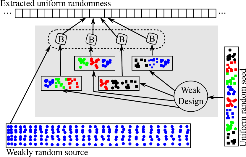
Figure 2: Interplay of components in Trevisan’s extractor. The weak design expands the initial seed into multiple smaller packets with certain overlap properties whose cumulative length can considerably exceed the seed length. Each is fed into a 1-bit extractor $B$, which distills a single random bit out of the global randomness for each packet. The bits are finally concatenated to form the extracted randomness. All components that make up Trevisan’s algorithm are highlighted in a grey box.

It turns out that there are many examples of one-bit extractors and weak designs that fulfil the requirements needed for the above procedure to work. Trevisan’s construction is therefore not really a single algorithm, but rather a recipe to combine different one-bit extractors and weak designs to generate a quantum-proof strong extractor. The exact choice of either building block (we also refer to them as primitives in the following) depends very much on the application and on the parameter regime of interest. Consequently, we decided to implement different possible choices and let the operator decide which ones to use. We now present two exemplary use cases that do especially highlight the need to prioritise between speed, entropy loss, and the assumptions on the initial randomness.

Suppose first that we have at our disposal a fast source providing very good random numbers, or equivalently, having a very high entropy. Ideally, we would like to extract all randomness, but since producing new random numbers is fast, we can allow a substantial entropy loss, concentrating on performance instead. In this case, the combination of the GF($p$)-weak design with the XOR one-bit extractor is the best choice, achieving a throughput of about 17 kbit/s on a normal notebook machine and about 160 kbit/s on a large workstation with 48 cores. The extractor can handle input lengths of several GiBits, which is also necessary since in these extreme cases only one percent of the available entropy is extracted. This means that the source needs to provide random numbers with a rate of about 20 Mibit/s. The required amount of seed for the one-bit extractor is 1.7 KiBit, which leads to a total seed of roughly 2.9 MiBit for 4 GiBit of input data.

If we consider a source of very low entropy and focus on small entropy loss rather than throughput, the optimal choice turns out to be the block weak design together with polynomial hashing for the one-bit extractor. It works for any lower bound on the entropy, has almost minimal entropy loss, and requires the shortest seed of all constructions. It is, however, much slower than the first combination: A throughput of only a few kbit/s is achieved on a notebook computer, or 70 kbit/s with 48 cores, albeit for a much shorter input length of $2^{16}$ bits: 100 bits are necessary for the one-bit extractor, which results in 10 KiBit of total seed for the standard weak design, and slightly less than 300 KiBit for the block weak design needed to extract nearly all the entropy.

These are just two examples, and proper performance measurements as well as a discussion on possible improvements and aspects of high-performance computing can be found in section V.

III Derivations

III.1 Trevisan’s extractor

III.1.1 Description

As briefly sketched in the previous section, Trevisan’s construction consists in applying multiple times the same one-bit extractor to the input string, using different weakly correlated seeds for each run. The seeds are chosen as substrings of some longer seed $y\in\{0,1\}^{d}$. Let $\{S_{i}\}_{i}$ be a family of sets such that for all $i$, $|S_{i}|=t$ and $S_{i}\subset[d]=\{1,\dotsc,d\}$. Then $y_{S_{i}}$ – the string formed by the bits of $y$ at the positions given by the elements $j\in S_{i}$ – is a string of length $t$. For a given one-bit extractor $C:\{0,1\}^{n}\times\{0,1\}^{t}\to\{0,1\}$, and such a family of sets $\{S_{i}\}_{i=1}^{m}$, Trevisan’s extractor is defined as the concatenation of the output bits of $C$ when used with the seeds $y_{S_{i}}$, namely

$$\operatorname{Ext}(x,y):=C(x,y_{S_{1}})\dotsb C(x,y_{S_{m}}).$$ (1)

The performance of the extractor naturally depends on the performance of the one-bit extractor, but also on the independence of the seeds used for each run of the one-bit extractor. Intuitively, the smaller the cardinality of the intersections of the sets $\{S_{i}\}$, the more randomness we can extract form the source, but the larger the seed. The exact condition is given in the following definition.

Definition III.1 (weak design Raz et al. (2002)).

A family of sets $S_{1},\dotsc,S_{m}\subset[d]$ is a weak $(m,t,r,d)$-design if

1. For all $i$, $|S_{i}|=t$.

2. For all $i$, $\sum_{j=1}^{i-1}2^{|S_{j}\cap S_{i}|}\leq rm$.

In the following, we refer to the parameter $r$ as the overlap of the weak design.

As an example, if we use a quantum-proof $(k,\varepsilon)$-strong extractor as one-bit extractor and a weak $(m,t,r,d)$-design, the construction given by (1) is a quantum-proof $(k+rm,m\varepsilon)$-strong extractor (see Lemma B.8). Thus, if $r=1$, Trevisan’s extractor has roughly the same entropy loss as the underlying one-bit extractor. Note also that the error $\varepsilon$ of the one-bit extractor is the error per bit for Trevisan’s construction.

III.1.2 Constructions overview

We always denote the input length by $n$, and the output length by $m$. We choose $\varepsilon$ in such a way that it corresponds to the error per bit for the final construction. We use $d$ to describe the seed length of Trevisan’s extractor and $t$ for the seed length of the underlying one-bit extractor. $r$ denotes the overlap of the weak design, and $k$ the min-entropy required in the source, which is often expressed as $k=\alpha n$.

In the following, we briefly summarize the constructions described in Sections III.2 and III.3. We take the input length $n$, output length $m$, and error per bit $\varepsilon$ to be fixed, and calculate the seed length $d$ and entropy needed in the source $k$ as functions of these three parameters.

Weak designs:

In Section III.2 we describe two weak designs, the first was originally proposed by Nisan and Wigderson Nisan and Wigderson (1994b), and has parameters $d=t^{2}$ and $r=2e$ for any prime power $t$ and any $m$. This means that the seed of the final construction is the square of the seed of the one-bit extractor, and the entropy loss induced by the weak design is $(2e-1)m\approx 4.436m$. The second construction iterates the first; it has a larger $d=at^{2}$ for

$$a=\mathopen{}\mathclose{{}\left\lceil\frac{\log(m-2e)-\log(t-2e)}{\log 2e-\log(2e-1)}}\right\rceil,$$ (2)

but $r=1$, i.e., the design does not cause any entropy loss.

XOR-code:

The XOR-code is a one-bit extractor, which simply computes the XOR of a substring of the input. With the two different weak designs, we find that the randomness and seed needed are

$$k =\gamma n+rm+6\log\frac{1+\sqrt{2}}{\varepsilon}+\log\frac{4}{3},$$

$$t =\frac{2\ln 2}{h^{-1}(\gamma)}\log n\log\frac{(2+\sqrt{2})}{\varepsilon},$$

$$d =t^{2}\text{ or }at^{2},$$

where $\gamma$ is a free parameter that influences the amount of extracted randomness and the length of the initial seed (details in Section III.3.1), and $a$ is given by Eq. (2). $h(p)=-p\log p-(1-p)\log(1-p)$ is the binary entropy function, and its inverse is defined on the interval $(0,1/2)$.

Lu’s construction:

This one-bit extractor selects a random substring of the input by performing a walk on an expander graph, and then hashes the result to one bit by taking the parity of the bitwise product with a random string. With the two different weak designs, we find that the randomness and seed needed are

$$k =h(\nu)n+rm+6\log\frac{2+\sqrt{2}}{\varepsilon}-2,$$

$$t =\log n+3c(\ell-1)+\ell,$$

$$c =\mathopen{}\mathclose{{}\left\lceil\frac{\log w}{2\log 5\sqrt{2}/8}}\right\rceil,$$

$$\ell =\mathopen{}\mathclose{{}\left\lceil\frac{8\log\varepsilon-8\log(2+\sqrt{2})}{\log(1-\nu+w)}}\right\rceil,$$

$$d =t^{2}\text{ or }at^{2},$$

where $\nu\leq 1/2$ is a free parameter, $a$ is given by Eq. (2), and $w$ is the solution to the equation

$$w\log w=(1-\nu+w)\log(1-\nu+w).$$

Polynomial hashing:

This constructions uses almost universal hash functions. With the two different weak designs, we find that the randomness and seed needed are

$$k =rm+4\log\frac{1}{\varepsilon}+6,$$

$$t =2\mathopen{}\mathclose{{}\left\lceil\log n+2\log\frac{2}{\varepsilon}}\right\rceil,$$

$$d =t^{2}\text{ or }at^{2},$$

where $a$ is given by (2).

III.2 Weak designs

The weak design construction we use (see Section III.2.1 for a description) is originally from Nisan and Wigderson Nisan and Wigderson (1994b), who proved that it is a standard design – a notion stronger than weak designs, originally used by Trevisan Trevisan (2001), but which Raz et al. Raz et al. (2002) showed to be unnecessary. Hartman and Raz Hartman and Raz (2003) proved that this construction is a weak $(m,t,r,d)$-design with overlap $r=e^{2}$ for a prime $t$, $d=t^{2}$, and $m$ a power of $t$. Ma and Tan Ma and Tan (2011) improved Hartman and Raz’s analysis, and showed that $r=e$ for any prime power $t$ and any $m$ which is a multiple of a power of $t$. However, for a practical implementation, we need a construction that is valid for any $m$. We prove in Appendix C.1 that this construction is a weak $(m,t,r,d)$-design for any prime power $t$, any $m$, and $r=2e$.

As mentioned in Section III.1, a larger overlap leads to a larger entropy loss. In Section III.2.2 we adapt an iterative construction of the basic design from Ma and Tan Ma and Tan (2011), to construct a new design with $r=1$. We prove in Appendix C.2 that this construction is correct.

III.2.1 Basic construction

In this section we describe a weak design construction, that is, we define a family of sets that satisfy the conditions of Definition III.1.

This construction makes use of polynomials over a finite field $\operatorname{GF}(t)$. Every set $S_{p}$ is indexed by one such polynomial $p:\operatorname{GF}(t)\to\operatorname{GF}(t)$. To construct a weak $(m,t,r,d)$-design we need $m$ sets, and therefore $m$ such polynomials, which we take in increasing order of their coefficients. For example, if $m=6$ and $t=2$, the polynomials are $\sum_{i=0}^{2}\alpha_{i}x^{i}$, with the coefficients $(\alpha_{2},\alpha_{1},\alpha_{0})$ taken in the following order: $(0,0,0)$, $(0,0,1)$, $(0,1,0)$, $(0,1,1)$, $(1,0,0)$, $(1,0,1)$. In general, the $n$th polynomial is given by $p(x)=\sum_{i=0}^{c}\alpha_{i}x^{i}$, with $\alpha_{i}=(n-1)/t^{i}\mod t$ and $c=\mathopen{}\mathclose{{}\left\lceil\frac{\log m}{\log t}-1}\right\rceil$.

The elements of the set $S_{p}$ are all the pairs of values $S_{p}:=\{(x,p(x)):x\in\operatorname{GF}(t)\}$. Each set thus has $|S_{p}|=t$ elements, and $S_{p}\subset[d]$ holds for $d=t^{2}$, where we map $[d]$ to $[t]\times[t]$ in the obvious way. We prove in Appendix C.1 that for all $m$ and $p$, this construction has $\sum_{\{q<p\}}2^{|S_{p}\cap S_{q}|}\leq 2em$, where by $\{q<p\}$ we mean the set of all polynomials that come before $p$.

III.2.2 Reducing the overlap

Note that any weak design can be viewed as a binary $(m\times d)$-matrix $W$, where the value $w_{ij}=1$ if $j\in S_{i}$. To construct a weak design with $r=1$, we will use the construction from Section III.2.1 repeatedly with different values $m_{j}$ (but the same $t$), obtaining designs $W_{\text{B},0},\dotsc,W_{\text{B},\ell}$. We then construct a new design $W$ by placing these in its diagonal, that is,

$$W=\mathopen{}\mathclose{{}\left(\begin{array}[]{ccc}W_{\text{B},0}&&\\ &\ddots&\\ &&W_{\text{B},\ell}\end{array}}\right).$$

Let $m$ and $t$ be fixed, and let $r^{\prime}=2e$ be the parameter from the basic construction. The number of calls to the basic construction is given by

$$\ell:=\max\mathopen{}\mathclose{{}\left\{1,\mathopen{}\mathclose{{}\left\lceil\frac{\log(m-r^{\prime})-\log(t-r^{\prime})}{\log r^{\prime}-\log(r^{\prime}-1)}}\right\rceil}\right\}.$$ (3)

And each design $W_{\text{B},i}$ is constructed with $m_{i}$ sets, defined as follows:

$$\begin{split}n_{i}&:=\mathopen{}\mathclose{{}\left(1-\frac{1}{r^{\prime}}}\right)^{i}\mathopen{}\mathclose{{}\left(\frac{m}{r^{\prime}}-1}\right)\qquad\text{for $0\leq i\leq\ell-1$},\\ m_{i}&:=\mathopen{}\mathclose{{}\left\lceil\sum_{j=0}^{i}n_{j}}\right\rceil-\sum_{j=0}^{i-1}m_{j}\qquad\text{for $0\leq i\leq\ell-1$},\\ m_{\ell}&:=m-\sum_{j=0}^{\ell-1}m_{j}.\end{split}$$ (4)

The weak design $W$ thus has $d=(\ell+1)t^{2}$. In Appendix C.2 we prove that this construction has $r=1$.

Figure 3 discusses the parameter behaviour of the block weak design.

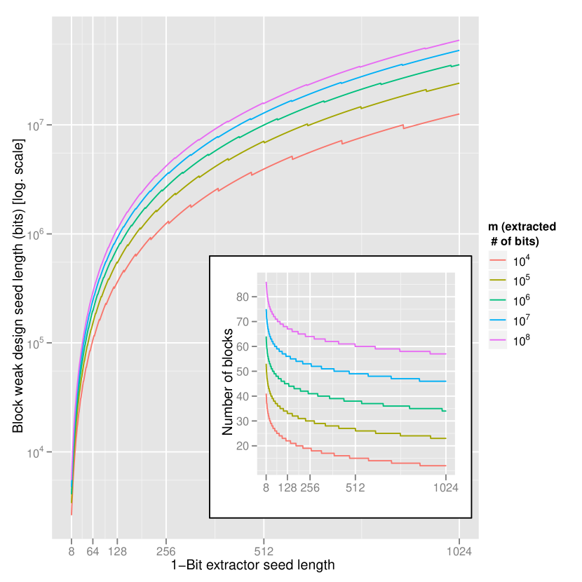
Figure 3: Total seed length required for the weak block design (based on an elementary design with $r=2e$) depending on the seed length of the 1-bit extractor. The inset shows the number of blocks – since the seed size for the block design depends linearly on the block number, this is also the seed overhead associated with the use of a block design. For typical parameters, the amount of seed grows by a factor of $50$.

III.3 One-bit extractors

III.3.1 XOR-code

This extractor computes the XOR for $\ell$ random positions of the input, it is thus an $\ell$-local extractor (see Appendix A for a precise definition). This construction is efficient to compute, but requires a seed of length $t\in O(\log n\log 1/\varepsilon))$, where $n$ is the input length and $\varepsilon$ the error of the construction, instead of the optimal $O(\log n+\log 1/\varepsilon)$. It also has an entropy loss linear in the input length.

Lemma III.2 (XOR-code (Impagliazzo et al., 2009, Theorem 41)).

For any $\varepsilon>0$, $n\in\mathbb{N}$ and $\ell\in[n]$, the function

$$C_{n,\varepsilon,\ell}:\ \{0,1\}^{n}\times[n]^{\ell}\to\{0,1\}$$

$$(x,i_{1},\dots,i_{\ell})\mapsto\bigoplus_{j=1}^{\ell}x_{i_{j}}$$

is a classical/proof $\ell$-local $(k,\varepsilon)$-strong extractor with $k=h\mathopen{}\mathclose{{}\left(\frac{\ln 2}{\ell}\log\frac{2}{\varepsilon}}\right)n+3\log\frac{1}{\varepsilon}+\log\frac{4}{3}$ and seed length $t=\ell\log n$, where $h(p)=-p\log p-(1-p)\log(1-p)$ is the binary entropy function.

By Lemma B.5, this construction is a quantum/proof $(k,(1+\sqrt{2})\sqrt{\varepsilon})$-strong extractor. And by Lemma B.8, if we use this in Trevisan’s construction, the final extractor is a quantum/proof $(k+rm,m(1+\sqrt{2})\sqrt{\varepsilon})$-strong extractor.

Let our source have min-entropy $H_{\min}(X|E)=\alpha n$. We want the entropy loss induced by this one-bit extractor to be roughly $\gamma n$, and need to find the appropriate $\ell$ for the desired value of $\gamma$ since $\gamma(\ell,\varepsilon)=h\mathopen{}\mathclose{{}\left(\frac{\ln 2}{\ell}\log\frac{2}{\varepsilon}}\right)$ for some $\gamma<\alpha$. Solving for $\ell$, we find $\ell(\gamma,\varepsilon)=\frac{\ln 2}{h^{-1}(\gamma)}\log\frac{2}{\varepsilon}$. This implies that $\gamma$ directly influences the length of the seed, which we discuss below. Since the inverse binary logarithm $h^{-1}(\cdot)$ is not analytically available, we need to resort to numerical techniques to determine the appropriate value of $\ell$ for a given $\gamma$. It is convenient to distinguish the experimental entropy deficiency $\alpha$ from the loss induced by the extraction procedure by introducing a parameter $\mu$ such that $\gamma=\mu\alpha$.

For $\varepsilon=\frac{\varepsilon^{\prime 2}}{(1+\sqrt{2})^{2}}$, Trevisan’s construction is a quantum $(k,\varepsilon^{\prime}m)$-strong extractor with $k=\gamma n+rm+6\log\frac{(1+\sqrt{2})}{\varepsilon^{\prime}}+\log\frac{4}{3}$. The seed of the one-bit extractor has length $t=\ell\log n=\frac{2\ln 2}{h^{-1}(\gamma)}\log n\log\frac{(2+\sqrt{2})}{\varepsilon^{\prime}}$, and the seed of the complete construction has length $d$.

Especially the choice of $\mu$ influences the behaviour of the XOR extractor. Figures 4, 5, and 6 depict and discuss the effect of the various chosen and inferred parameters.

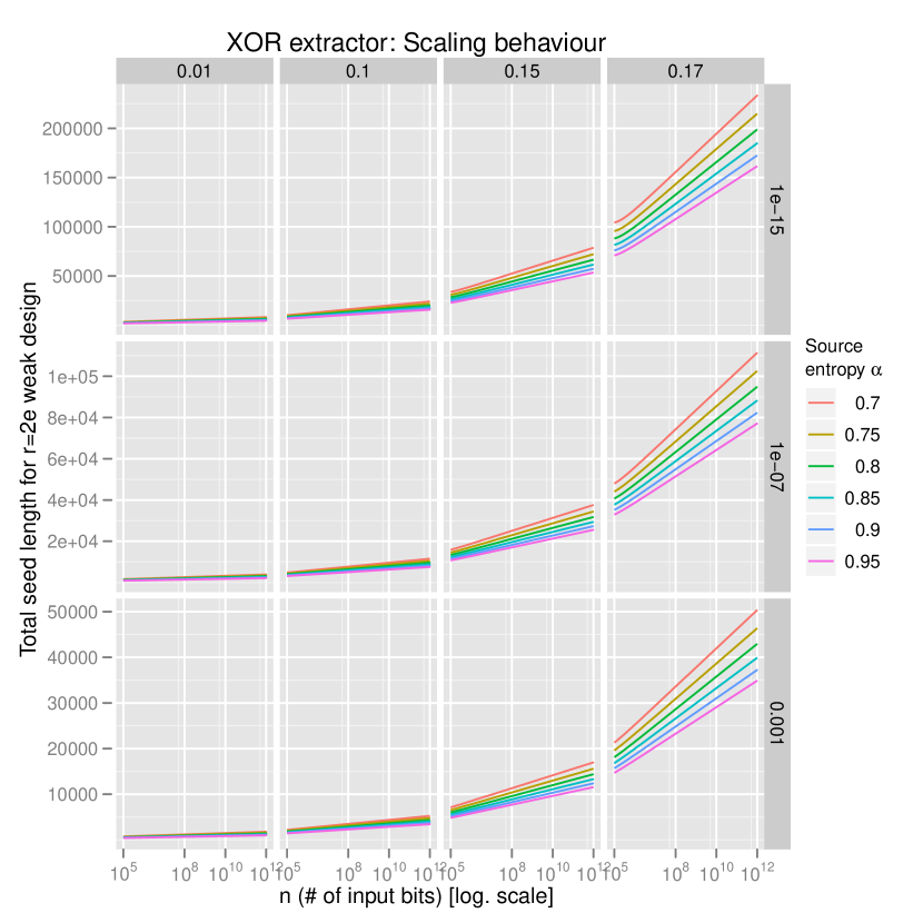
Figure 4: XOR parameter behaviour overview. $\mu$ varies per column, $\varepsilon$ per row. The influence of the initial source entropy $\alpha$ is mostly negligible, especially for small values of the extraction ratio $\mu$. However, there is a drastic increase in seed size for $\mu>0.16$, which restricts the XOR method to a practical upper bound of the extraction ratio of about 10% of the source entropy.

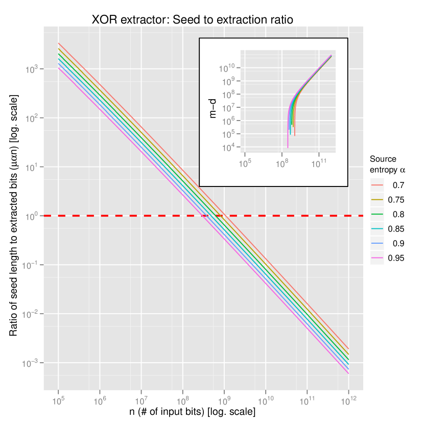
Figure 5: Ratio between output size and seed length for various input sizes. The parameters $\mu=0.05$ and $\varepsilon=10^{-7}$ are fixed for this computation. A ratio of 1, indicated by a dashed red line, denotes the parameter regime where the amounts of extracted bits and the seed spent coincide; for values exceeding this threshold, the particular advantages of Trevisan’s construction over two-universal hashing prevail because the ratio is better than what can be achieved with the latter approach. Recall, though, that the seed acts as a catalyst that can be included in the final randomness since the extracted bits are independent of the seed.
The initial source entropy $\alpha$ accounts for a variation of about one order of magnitude of the extraction threshold. As a rule of thumb, the break-even point is at input sizes of roughly of $10^{9}$ bits, which amounts to approximately $2^{30}$ bytes (roughly 1 GiB) of data.
The inset shows the number of extracted bits less the seed spent.

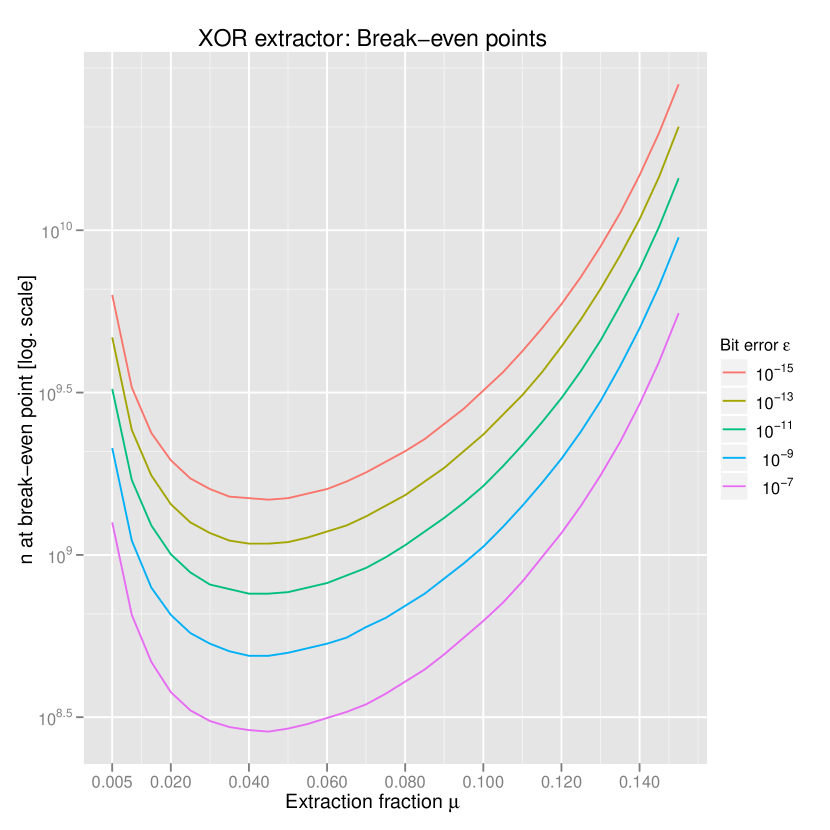
Figure 6: Break-even points (i.e., minimal input length for which the amount of extracted randomness exceeds the required seed size) for varying values of $\mu$ and $\varepsilon$. The parameter $\alpha$ is fixed to 0.8. As a rule of thumb, $\mu=0.05$ is close to the optimal value irregardless of the error parameter $\varepsilon$).

III.3.2 Lu’s construction

Lu Lu (2004) shows how to construct a local one-bit extractor, i.e., an extractor for which each bit of the output only depends on a subset of the input bits. He then uses his one-bit extractor in Trevisan’s construction. Here, we adapt the parameters of his construction to build a quantum/proof extractor.

Lu’s extractor proceeds in two steps. The first consists in selecting a substring of the input; the second hashes this string to one bit. To select the substring of the input, he performs a random walk on a $g$-regular graph – a graph in which every vertex is connected to exactly $g$ other vertices.

Recall that a graph $G$ is uniquely identified by its vertices and edges, and is consequently specified by $G=(V,E)$, where $V$ is the vertex set and $E$ the edge set. An alternative representation of more importance in our context is the adjacency matrix. For a graph with $n$ vertices, this is an $n\times n$ matrix in which the entry $a_{ij}$ denotes the number of edges from vertex $i$ to vertex $j$. The diagonal is typically filled with ones; since the graphs considered here are undirected (i.e., the direction of edges is not taken into account, only the fact that two vertices are connected), the adjacency matrix is symmetric.

The eigenvalues of the adjacency matrix are referred to as eigenvalues of the graph. For our purpose, the ratio between the second largest and largest eigenvalue plays an important role, and is labelled as $\lambda$. Graphs with a small $\lambda$ are called expander graphs, and are common objects in pseudo-randomness generation, see Ref. Goldreich (2011) for a review.

For an input string of length $n$, we choose a graph with $n$ vertices, so that each vertex corresponds to a bit position of the string. Let $(v_{1},\dotsc,v_{\ell})$ be the vertices visited during a walk of $\ell$ steps. We select the $\ell$ corresponding bits of the input $x$, that is, $(x_{v_{1}},\dotsc,x_{v_{\ell}})$, and then hash it by computing the parity of the bitwise product of this string with a random seed $\beta\in\{0,1\}^{\ell}$. The output is thus $z=\bigoplus_{i=1}^{\ell}\beta_{i}x_{v_{i}}$.

Lu Lu (2004) proves that the concatenation of the output bits $z$ for all possible seeds is a $(\delta,L)$-list decodable code with

$$L=\frac{2^{h(\nu)n}}{2\delta^{2}},$$ (5)

for a $\nu\leq 1/2$ given by

$$\nu=1+\lambda^{2}-\delta^{\frac{4}{\ell}}.$$ (6)

Since $\delta^{\frac{4}{t}}<1$, (6) can only be satisfied if $\lambda^{2}<\nu$. This can be obtained by taking as expander graph $G$ a given construction $G_{0}$ to the power $c$. $G$ is defined as the graph with adjacency matrix $A=A^{c}_{0}$, where $A_{0}$ is the adjacency matrix of $G_{0}$. We then have $\lambda=\lambda_{0}^{c}$. A random walk of length $\ell$ on $G_{0}^{c}$ is equivalent to a random walk of length $\ell c$ on $G_{0}$, in which only the first of every $c$ steps is remembered, and the others deleted Hoory et al. (2006).

To construct the regular expander graph $G_{0}$, we employ an algorithm reviewed in Ref. Goldreich (2011). Let us only summarise the essential facts here:

• The construction is restricted to degree $g=8$, and the ratio between the second-largest and largest eigenvalue can be shown to be $\lambda=5\sqrt{2}/8\approx 0.884$.

• It is possible to compute the graph for all dimensions (i.e., number of nodes) that can be expressed as $\ell^{2}$ for $\ell\in\mathbbm{N}$. This restriction is much more relaxed than for other constructions, and does not pose any problems in real applications. Formally, the vertex set of the graph is defined on $\mathbbm{Z}_{\ell}\times\mathbbm{Z}_{\ell}$. Each vertex $\langle x,y\rangle\in\mathbbm{Z}_{\ell}\times\mathbbm{Z}_{\ell}$ is connected to the vertices $\langle x\pm 2y,y\rangle$, $\langle x\pm(y+1),y\rangle$, $\langle x,y\pm 2x\rangle$, and $\langle x,y\pm(2x+1)\rangle$, which uniquely defines the edges. Notice that the arithmetic must be performed modulo $\ell$, so the computationally (comparatively) cheap additions and multiplications are unfortunately accompanied by an expensive modulo division.

• The complete graph does not need to be computed in advance, but can be constructed during the random walk, and using a constant amount of space.

For a given $\nu$, we choose $c$ and $\ell$ which minimize the number of steps $c\ell$. By setting $w:=\lambda_{0}^{2c}$ and taking the derivative of $c\ell$ with respect to $w$, we find that minimum is obtained for the $w$ which is the solution of the equation

$$w\log w=(1-\nu+w)\log(1-\nu+w).$$

The number of steps on the expander graph is then given by $c=\mathopen{}\mathclose{{}\left\lceil\frac{\log w}{2\log\lambda_{0}}}\right\rceil$ and $\ell=\mathopen{}\mathclose{{}\left\lceil\frac{4\log\delta}{\log(1-\nu+w)}}\right\rceil$.

The walk on the $g$-regular graph requires $\operatorname{nb}(n)$ bits of seed to choose the first vertex, and $c(\ell-1)\log g$ bits for the direction of the walk for each following step. The final hashing uses $\ell$ bits of seed, for a total of $t=\operatorname{nb}(n)+c(\ell-1)\log g+\ell$.

From Lemma B.3 and (5), Lu’s one-bit extractor is a classical-proof $(h(\nu)n+3\log\frac{1}{\delta}-2,2\delta)$-strong extractor. By Lemma B.5 it is quantum-proof $(h(\nu)n+3\log\frac{1}{\delta}-2,(2+\sqrt{2})\sqrt{\delta})$. And from Lemma B.8, when used with a weak $(m,t,r,d)$-design, Trevisan’s construction is a quantum-proof $(k,m\varepsilon)$-strong extractor with $k=h(\nu)n+rm+6\log\frac{2+\sqrt{2}}{\varepsilon}-2$.

Unfortunately, Lu’s construction is not useful in a practical setting owing to its unfortunate parameter scaling: The number of random walk steps increases considerably with decreasing parameter $\nu$, see Figure 7. However, as Figure 8 shows, small values of $\nu$ are required for even tiny extraction fractions. Overall, this makes the construction reach parameter realms where it is preferable over two-universal hashing functions (namely, when the length of the extracted bits exceeds the amount of initial seed) only rarely, as Figure 9 shows.

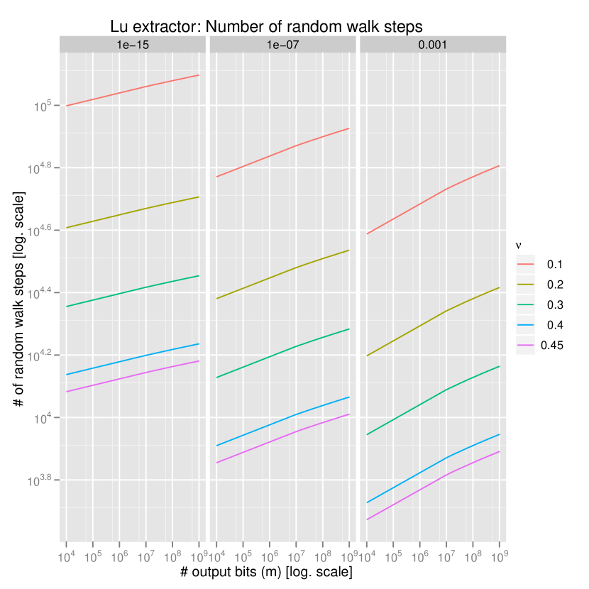
Figure 7: Number of random walk steps required in Lu’s construction in dependent on the output length and the parameter $\nu$.

Figure 8: Dependency between parameters $\nu$ and $\mu$ for Lu’s construction. The largest value of $\nu$ that satisfies the boundary conditions on the available entropy given in Section III.3.2 was determined numerically.

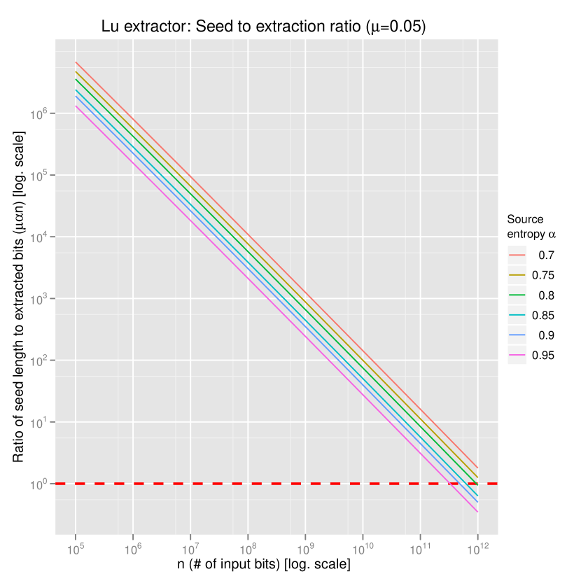
Figure 9: Comparision of seed size and output size for Lu’s construction. The interesting regime is only reached in very rare cases.

III.3.3 Polynomial hashing

Renner Renner (2005) proved that universal₂ hash functions are good extractors. Tomamichel et al. Tomamichel et al. (2011) showed that the same holds for $\delta$-almost universal₂ ($\delta$-AU₂) hash functions, given that $\delta$ is small enough. For the range of $\delta$ that build good extractors, almost universal₂ hashing requires a seed of length $\Omega(m+\log n)$, where $n$ is the input and $m$ the output length. This seed is too large for many applications; however in the case of one-bit extractors, this reduces to $\Omega(\log n)$, and is achievable with the construction we describe here.

This construction is in fact the concatenation of two hash functions, and uses a seed of length $2\ell$, where $\ell$ will be specified later. The first is known as polynomial hashing – or alternatively as a Reed-Solomon code, because the concatenation of the hashes for all seeds corresponds to the encoding of the input with a Reed-Solomon code. We partition the input string $x\in\{0,1\}^{n}$ in blocks $x=(x_{1},\dotsc,x_{s})$, each of length $\ell$ (if necessary, we pad the last string $x_{s}$ with $0$s). We view each block as an element of a field $x_{i}\in\operatorname{GF}(2^{\ell})$, and evaluate the polynomial

$$p_{\alpha}(x)=\sum_{i=1}^{s}x_{i}\alpha^{s-i},$$

where $\alpha\in\operatorname{GF}(2^{\ell})$ is the first half of the seed. This family is $\frac{s-1}{2^{\ell}}$-AU₂. Stinson (1995)

Since the $\delta$ of polynomial hashing is too large (relative to the output length) to build an extractor, we combine it with another hash function – sometimes referred to as a Hadamard code, as the concatenation of the outputs over all seeds corresponds to the Hadamard encoding. This hash function computes the parity of the bitwise product of $p_{\alpha}(x)$ and the second half of the seed, $\beta\in\{0,1\}^{\ell}$. The output is thus $z=\bigoplus_{i=1}^{\ell}\beta_{i}p_{\alpha}(x)_{i}$. Since this hash function is $\frac{1}{2}$-AU₂, by (Stinson, 1994, Theorem 5.4) the combination of the two is $\delta$-AU₂ with $\delta=\frac{1}{2}+\frac{s-1}{2^{\ell}}$.

Choosing $\ell=\lceil\log n+2\log 1/\varepsilon^{\prime}\rceil$, $s=\lceil n/\ell\rceil$ we get

$$\delta=\frac{1}{2}+\frac{s-1}{2^{\ell}}<\frac{1}{2}+\frac{n}{2^{\ell}}\leq\frac{1}{2}+\varepsilon^{\prime 2}.$$

From Theorem B.7, this is a quantum/proof $(4\log\frac{1}{\varepsilon}+2,2\varepsilon^{\prime})$-strong extractor. And plugging this in Trevisan’s construction with a $(m,2\ell,r,d)$-design and $\varepsilon=2\varepsilon^{\prime}$, we get from Lemma B.8 a quantum/proof $(4\log\frac{1}{\varepsilon}+6+rm,m\varepsilon)$-strong extractor. The seed of the one-bit extractor has length $t=2\ell=2\lceil\log n+2\log 2/\varepsilon\rceil$, and the seed of the complete construction has length $d$.

Figure 10 discusses the parameters of the polynomial hashing extractor.

Figure 10: Polynomial hashing parameter overview (calculations are for $r=2e$). The parameters are easy to evaluate because there is no dependence on $\alpha$, and there is also no extraction factor $\mu$—the extractor works equally well for high- and low-entropy sources. The required seed is consistently small (shown in the bottom inset); it increases linearly as $\varepsilon$ decreases exponentially.
The degree of the polynomial that needs to be evaluated is the crucial factor. Even for small inputs like $n=10^{6}$, corresponding to roughly 1 MiB of data, the degree is $\approx 10000$. Since the polynomial needs to be evaluated for every extracted bit, this makes the polynomial hashing extractor an unsuitable choice for performance intensive scenarios.
The top inset shows the regime in which the extractor delivers more bits than initially invested for the seed. It outperforms two-universal hashing for a very wide range of parameters.

.

IV Implementation

IV.1 Implementation Architecture

We now turn our attention to describing the implementation of the Trevisan extraction framework by first outlining the software architecture, that is, the high-level conceptual point of view, followed by a discussion of some important implementation details and notes on how to add new primitives to the infrastructure. While many important details are still omitted for the sake of brevity, the full source code is available at https://github.com/wolfgangmauerer/libtrevisan for inspection and modification. Besides instructions on how to build the code, the website also contains detailled information on how to use the program, which we will not discuss here any further.

IV.1.1 Architecture

The architecture was designed to satisfy two particular constraints: Correctness and maximum throughput. To achieve the latter, we use C++ to implement all performance-critical parts, since the language is statically compiled and does not require any intermediate layers that add runtime penalties to interpreted or byte-compiled languages like, for instance, Matlab, but still allows us to maintain a clean and extensible design based on modern software engineering techniques Stroustrup (2000). The implementation is portable across a wide range of machines from laptops to high performance computing (HPC) machines, and also provides opportunities to benefit from low-level capabilities of recent CPUs, for instance to accelerate bit-level manipulations. We have tested the code on Linux and MacOS machines.

To ensure correctness of the calculations, we base the implementation on independent libraries (NTL Shoup (2005) and OpenSSL OpenSSL Project (2003) for working with finite fields of arbitrary size) that can be selected at compile time. Checking that both variants arrive at the same results for identical parameter sets increases the faith in the reliability of the calculations. Another means to ensure code correctness is given by a large number of invariants and sanity checks that are spread all across the implementation. To not compromise the performance goals, it is possible to deactivate the checks at compile time so that they incur no runtime penalty.

Another major design decision is the focus on multi-core machines: Nowadays, machines with only a single core are a rare exception, and algorithms that are limited to only one thread of execution voluntarily sacrifice a large fraction of the available computational power, which is obviously not desirable in a high-performance setting. We use the threading building blocks library Reinders (2007) as basis for the implementation, which allows for fine-tuning the distribution of work across the system ressources in a precise manner. We also employ a mostly lock-free architecture (see, e.g., Ref. Herlihy and Shavit (2008) for a review) that avoids any computation stalls due to the need for synchronised communication between computation elements.

The code also contains parts that are not performance-critical, for instance calculating the parameters from given user settings. This is conveniently done in very high-level languages that allow for working in abstract terms without having to consider any details of the underlying machine architecture. To this end, we have integrated the possibility to call code written in the R language (using the techniques provided by Ref. Eddelbuettel and Francois (2012); see R Development Core Team (2011) for an overview about R), which enjoys widespread use in statistical data processing and machine learning.

It is also possible to compute the weak design ahead of time, store it on disk and re-use it for multiple runs of the extractor – since computing the weak design is a deterministic operation that does not require any randomness, this is admissible to do. In matrix representation, a weak design for output length $m$ and a total seed length $d$ is an element $\mathbb{F}_{2}^{m\times d}$. Each row contains $t$ ones and $d-t$ zeroes, so the matrix fill for the standard design is $\frac{mt}{m(d-t)}\approx 1/t$. A total seed of 50 KiBit, for instance, amounts to a fill of about 0.5%, which exceeds the threshold for typical sparse matrix techniques to pay off Golub and van Loan (1996). We found the data transfer times from the underlying block device to be longer than the time required to compute the weak design on the fly, albeit this may change with the availability of high-speed storage. For the block weak design, the situation is more favourable since only the basic design needs to be stored, and the remaining elements can be reconstructed with very little computational effort.

Finally, we emphasise that the code can either be used in stand-alone mode (also including a dry-run mode for parameter estimation), or as a library as part of a larger project.

IV.1.2 Implementation details

Weak designs and one-bit extractors are implemented as C++ classes derived from mixed interface/implementation-type base classes. Trevisan’s algorithm solely operates on the base class objects using dynamic polymorphism, and does not require any knowledge about the internal structure of the primitives.

The source code contains full information on how to implement and integrate new primitives, so we only summarise briefly what methods need to be provided.

Weak designs need to be derived from class weakdes, and must implement

• compute_Si(uint64_t i, vector indices) – compute the $i$th index set, and store the results in indices.

• compute_d() – compute the required amount of initial seed.

• get_r() – report the overlap $r$ to the higher-level algorithms.

Optionally, the function set_params(uint64_t, uint64_t m) can, but need not be implemented to initialise the parameters required for all weak designs.

Determining $d$ from $t$ seems straightforward, but is accompanied by constraints – the $\operatorname{GF}(2^{x})$ based weak design, for instance, only works for values of $t$ that can be represented as a power of 2, so the design typically needs to choose larger values (resulting in more initial seed) than requested.

One-bit extractors need to be derived from class bitext, and must implement

• num_random_bits() – compute the amount $t$ of initial seed bits required for every extracted bit.

• compute_k() – determine the minimal source entropy required by the extractor for the parameter set under consideration.

• extract(void *initial_rand) – extract one bit using the provided subset of the initial randomness.

There are also generic functions to assign global randomness and other generic parameters to the 1-bit extractor. They can, but need not be provided by an implementation.

On the lower layers, the implementation was designed to use elementary machine arithmetic (as opposed to software-based multi-precision arithmetic) whenever possible; this is an obvious precondition for an implementation with good performance. In all performance critical operations, logarithms are not computed using floating point, but with integer operations since usually only floor or ceiling of the result is required.

The code uses a fixed-width integer data type with 64 bits to represent potentially large quantities like the number of input bits. It is important to note that the width of the index data type sets an upper bound on the amount of randomness that can be handled by the code, namely to $2^{w-3}$ bytes (for $w=32$ respectively $w=64$), which corresponds to $2^{w}$ bits (the datum is used as an index into a bit field, and this field need not be representable by a machine quantity). Since contemporary 64-bit machines cannot handle more than $2^{48}$ bytes owing to virtual address space management limits Mauerer (2008), the choice does not introduce any additional limits. To process large amounts of randomness (multiple gigabytes), 64 bit machines and a 64-bit kernel running on the machine are required, which the code assumes to be the default setting.

IV.2 Algorithms

In the following, we give a concise description of all algorithms in a form that is helpful for actual implementations—in some contrast to the previously given descriptions that focus more on mathematical clarity, we provide recipes in a pseudo-formal language that is close enough to many contemporary imperative and object-oriented programming languages, yet still sufficiently abstract to avoid hiding the algorithmic core behind technical side-work. Although each algorithm can be captured with very few statements, we remark that a practical implementation needs to account for many non-trivial technical issues; our reference implementation published as a part of this paper comprises about 5000 lines of source code.

IV.2.1 Trevisan’s extractor

The Trevisan algorithm is independent of the type of weak design and bit extractor used; only the inferred parameters depend on the specific properties of the components:

1:procedure Trevisan(WD, Ext, $n,m,\mu,\alpha,\varepsilon,\varrho^{\text{i}},\varrho^{\text{d}}$)

2:     $t\leftarrow\text{{Ext}}.\text{{InputSize}}(n,m,\mu,\alpha,\varepsilon)$

3:     $d\leftarrow\text{{WD}}.\text{{InputSize}}(t)$

4:     Reserve space for $m$ bits in $\varrho^{\text{o}}$

5:     Reserve space for $t$ numbers $\in[d]$ in $S$

6:

7:     for $i\leftarrow 0,m-1$ do$\triangleright$ Data parallel

8:         $S\leftarrow\text{{WD}}.\text{{computeS}}(i)$

9:         $b\leftarrow 0$

10:         for $j\leftarrow 0,t-1$ do

11:              $b_{j}\leftarrow\varrho^{\text{i}}_{S_{j}}$ $\triangleright$ Indices refer to bits

12:         end for

13:         $\varrho^{\text{o}}_{j}\leftarrow\text{{Ext}}.\text{{extract}}(b,\varrho^{\text{d}}$)

14:     end for

15:

16:     return $\varrho^{\text{o}}$

17:end procedure

The components WD and Ext may impose boundary conditions on the parameters; for instance, the single-bit seed length $t$ must be a power of a prime number for the weak designs implemented in this paper.

IV.2.2 Weak Designs

Construction of Hartman and Raz

The weak design of Hartman and Raz is based on evaluating polynomials over finite field; recall from Section III.1.2 that the dimension of the field needs to be a power of a prime number. We have implemented two variants: One based on the extension field $\mathbbm{F}=\operatorname{GF}(2^{x})$, and one based on the prime field $\mathbbm{F}=\operatorname{GF}(p)$. The bit extractors can require arbitrary values of $t$ that are not necessarily compatible with the constraints of the weak design. In this case, $t$ needs to be increased to the next possible value $t^{\prime}$ that can be provided by the weak design. Consequently, we need to distinguish between $t$, which represents the value that can be provided by the weak design, and $t^{\text{req}}$, which is the value originally requested by the bit extractor. It necessarily holds that $t\geq t^{\text{req}}$.

The basic algorithm for both finite fields is as follows (indices in square brackets denote bit selections):

1:procedure HR.ComputeS($\mathbbm{F},i,m,t$)

2:     $c\leftarrow\lceil\frac{\log m}{\log t}-1\rceil$

3:     for $j\leftarrow 0,c$ do $\triangleright$ Prepare polynomial coefficients

4:         $\alpha_{j}\leftarrow i[j\cdot\operatorname{nb}(t),j+\operatorname{nb}(t)-1]\mod t$

5:     end for

6:

7:     for $a=0,a<t^{\text{req}}$ do

8:         $b\leftarrow\sum_{j}\alpha_{j}a^{j}$

9:         $S^{a}_{i}[\log(t),2\cdot\log(t)-1]\leftarrow b$

10:         $S^{a}_{i}\leftarrow S^{a}_{i}\cdot a$

11:         $S^{a}_{i}\leftarrow S^{a}_{i}\mod|\mathbbm{F}|$

12:     end for

13:

14:     return $S$

15:end procedure

For a field of prime dimension $p$, all calculations are performed modulo $p$. Notice, though, that it is not sufficient to simply divide by $p$ after any multiplication (or addition/subtraction) has been performed, because this can easily lead to intermediate results that exceed the maximal bit width available in hardware. Multiplying two 40-bit numbers, for instance, can result in an 80-bit value, which exceeds the word size of 32 and 64 bit machines. A naïve solution could fall back to using arbitrary-precision software arithmetic, which is unfortunately much slower than native machine hardware arithmetic. Consequently, we use have made sure to use algorithms that avoid intermediate overflows and can work with multiplicands of up to $61$ bits, which is sufficient for our purposes. See the source code or Ref. Arndt (2010) for details.

For the extension field $\operatorname{GF}(2^{m})$, it is not sufficient to perform a simple division of arithmetic results by a scalar to satisfy the constraints of the finite field. Instead, all elements of the field are formally interpreted as polynomials over the binary field, and arithmetic operations are performed modulo an irreducible polynomial that needs to be constructed dependent on the field order. It can be shown (see, e.g., Ref. Shoup (2005)) that for every field order, an irreducible polynomial of order 3 or 5 exists, so calculations can be optimised for these cases.

Block Weak Design

The block weak design is based on a basic design whose matrix representation is re-used multiple times as part of the total weak design—once the matrix representation of the basic design is known, it is possible to construct the complete design by placing sub-matrices of the basic design matrix on the diagonal of a larger matrix. One possible implementation could thus use sparse matrix techniques to store the basic design in memory, and derive all other blocks from this representation.

When the basic design is not represented by a matrix, but as vectors of indices, it is possible to compute the content of $W_{\text{B},j}^{k}$ from the basic design row $W_{\text{B},0}^{k}$ by adding $j\cdot t^{2}$ to all values of the set $S$ corresponding to the matrix row. Since it is possible to re-arrange the rows of $W$ without changing the properties of the weak design, we use a suitable permutation (derived from the data in Eq. (4), see the source code for details) of the rows of $W$ such that all rows that originate from the same row of the basic design are adjacent to each other, which allows us to cache calls to the basic construction. Since the design is traversed from row to row in the Trevisan algorithm, the permuted row order minimises calls to the basic construction.

1:procedure BWD.computeS(WD, $i,i^{\text{c}},S^{\text{c}},t$)

2:     Infer $j,k$ from $i$

3:     if $k\neq i^{\text{c}}$ then

4:         $i^{\text{c}}\leftarrow k$

5:         $S\leftarrow\text{{WD}}.\text{{computeS}}(i^{\text{c}})$

6:

7:         for $\zeta\leftarrow 0,t-1$ do $\triangleright$ Fill cache

8:              $S^{\text{c}}_{\zeta}\leftarrow S_{\zeta}$

9:         end for

10:     else

11:         for $\zeta\leftarrow 0,t-1$ do

12:              $S_{\zeta}\leftarrow S^{\text{c}}_{\zeta}+j\cdot t^{2}$

13:         end for

14:     end if

15:

16:     return $S$

17:end procedure

IV.2.3 1-Bit extractors

Finally, we discuss the algorithms used for the 1-bit extractors implemented as part of this paper.

XOR Code

An implementation of the XOR code requires to derive the parameter $l$ from the experimental parameters; since this can be achieved by a standard numerical optimisation, we will not discuss a formal algorithm here, but refer the reader to the source code for the details. The algorithm itself is compact:

1:procedure XOR.extract($\varrho^{\text{i}},\varrho^{\text{d}}$)

2:     $r\leftarrow 0$

3:     for $i\leftarrow 0,l-1$ do

4:         $\zeta\leftarrow\varrho^{\text{i}}[i\cdot\operatorname{nb}(n-1),(i+1)\cdot\operatorname{nb}(n-1)-1]$

5:         $r\leftarrow r\oplus\varrho^{\text{g}}[\zeta]$

6:     end for

7:     return $r$

8:end procedure

Polynomial Hashing

The algorithm to perform polynomial hashing based on a concatenation of a Reed-Solomon and a Hadamard code is as follows:

1:procedure RSH.extract($\varrho^{\text{i}},\varrho^{\text{d}},n,\varepsilon$)

2:     $\zeta\leftarrow 0$, $l\leftarrow\lceil\log n+2\log 2/\varepsilon\rceil$

3:     $s\leftarrow\lceil n/l\rceil$

4:

5:     Pick irreducible polynomial for $\operatorname{GF}(2^{l})$

6:     for $i\leftarrow 0,s-1$ do $\triangleright$ Determine coefficients

7:         $c_{i}\leftarrow\varrho^{\text{g}}[i\cdot l,(i+1)\cdot l-1]$

8:     end for

9:

10:     $\alpha\leftarrow\varrho^{\text{d}}[0:l-1]$ $\triangleright$ Reed-Solomon step

11:     $r\leftarrow\sum_{i=1}^{s}c_{i}\alpha^{s-i}$ $\triangleright$ Computed over $\operatorname{GF}(2^{l})$

12:

13:     $b\leftarrow 0$ $\triangleright$ Hadamard step

14:     for $j\leftarrow 0,l-1$ do

15:         $b\leftarrow b\oplus(\varrho^{\text{i}}[l+j]\cdot r[j])$

16:     end for

17:

18:     return $b$

19:end procedure

Since the length of the global randomness is considerably exceeds the bit length of the largest quantity representable with elementary machine data types in all but the most pathological cases, evaluation of the polynomial has to be performed using arbitrary precision software arithmetic.

There are two obvious optimisations: The global randomness does not change across invocations of the RSH extractor, so it is possible to compute the coefficients of the polynomial once, and re-use the results in subsequent evaluations. In a practical implementation, it is also more efficient to use Horner’s rule for evaluating the polynomial Knuth (1997) instead of performing the straight-forward evaluation shown in the algorithm.

The final parity calculation is not done using single-bit operations in the actual implementation, but is split into two steps: Firstly, the logical “and” operation is computed block-wise on machine-word sized blocks. Secondly, the parity operation is built on special-purpose machine operations (or compiler intrinsics) to count the number of bits set in the result of the “and” operation. The parity can then be derived by checking if the bit count is even or odd.

Lu’s construction

The algorithm for Lu’s extractor based on a random walk on an expander graph is as follows (we do not discuss how the optimisations required to determine the parameters $c$ and $l$ are performed; see the source code for details):

1:procedure LU.extract($\varrho^{\text{i}},\varrho^{\text{d}},c,l$)

2:     $v\leftarrow\varrho^{\text{i}}[0:\zeta-1]$ $\triangleright$ Initial node

3:     $r\leftarrow 0$, $b\leftarrow 3$ $\triangleright$ 3 bits to represent an edge

4:     $w\leftarrow\varrho^{\text{i}}[\zeta:\zeta+c(l-1)\cdot b-1]$

5:     $s\leftarrow\varrho^{\text{i}}[\zeta+c(l-1)\cdot b:]$

6:

7:     for $i\leftarrow 0,c-1$ do

8:         $r\leftarrow r\oplus(\varrho^{\text{d}}[v]\cdot s[i])$

9:

10:         for j=0, l-2 do $\triangleright$ Random walk

11:              $e\leftarrow w[(i(l-1)+j)\cdot b,(i(l-1)+j+1)\cdot b-1]$

12:              $v\leftarrow\text{{next.vertex}}(v,e)$

13:         end for

14:     end for

15:     $r\leftarrow r\oplus(\varrho^{\text{d}}[v]\cdot s[c])$

16:

17:     return $r$

18:end procedure

$\zeta$ denotes the number of bits required to store the index of a node. Function $\text{{next.vertex}}(v,e)$ computes the value of the next vertex given the current vertex and the next edge; it is a straight-forward translation of the calculation rule given earlier in Section III.3.2.

Most of the implementation complexity for the Lu expander stems from the need to select subsets of bit strings. To simplify distributing the initial randomness provided by the weak design into three components as shown above, the actual implementation assumes that the contributions start on indices that are evenly divisible by the bit width of the data type used to represent edges. This simplifies the implementation, but implies that a slightly larger amount of randomness than theoretically possible is required, albeit the increase is only by a negligible additive factor.

V Runtime comparison

Owing to the many aspects—throughput, scalability, weak design versus extractor performance, parameter ranges, machine characteristics, among others—involved in determining code performance, and because of the large number of combinations of primitives, it is neither possible nor reasonable to present measurements for all cases (since the full sources are available, measurements for a particular case of interest can be easily conducted by interested parties). Instead, we focus on a selection of measurements that describe cases of typical experimental interest. We use two machines to run the tests; detailled technical specifications are shown in Table 1. One machine is a standard Laptop (MacBook Air) that allows for testing the performance on an average personal computer, and serves as an apt comparison basis to the machine used for the measurements in Ref. Ma et al. (2012). The second machine is a sizeable workstation that gives an indication for the behaviour in high-performance computing scenarios, or when one is willing to spend substantial computational effort on the post-processing, for example in scenarios in which the highest possible security is the foremost priority.

Machine	CPU	# CPUs	Cores/CPU	Threads/core	$\Sigma$ Threads	RAM [GiB]	Kernel
Laptop	Intel Core i5	1	2	2	4	4	Darwin 11.4.0
	1.6 Ghz
Workstation	AMD Opteron	8	6	1	48	32	Linux 3.0
	1.9 Ghz

Table 1: Machines deployed in the benchmark measurements.

The measurement results are shown in Figures 11, 12, 13, 14, and 15; refer to the captions for a detailled discussion of the results.

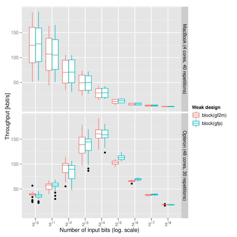
Figure 11: Scaling behaviour of RSH with a block design for varying input lengths. For a small number of CPUs, performance degrades considerably with increasing input length, as expected for a non-local extactor. Good throughput (more than 100 kbit/s) is only obtained fo very small input sizes ($2^{12}$ is only 4KiBit of data!) for which the required amount of initial seed drastically exceeds the extracted amount of randomness.
With many cores, the achieved speed-up does initially not compensate the overhead for setting up and performing parallel operations, so the throughput increases to a local maximum, and then decreases as expected with larger input lengths. Consequently, it is not just sufficient to add more CPUs for a given scenario to increase throughput; practical book-keeping tasks and technical aspects can easily dominate the actual problem. In particular, this implies that purely technical improvements like porting the processing to massively parallel approaches like GPU computing will not automatically resolve all performance needs; a proper choice of primitives for given requirements is essential, which is only possible with a framework that allows for flexibly combining these primitives.

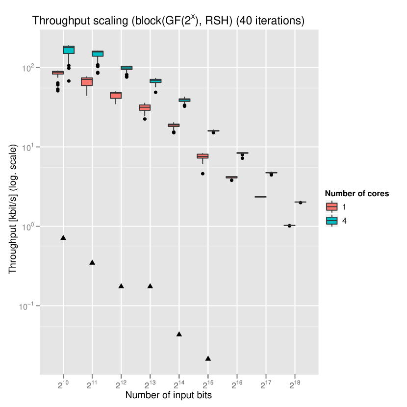
Figure 12: Throughput comparison of our results (obtained on a laptop, represented by boxplots) with the results obtained by Ma et al. (represented by triangles) for the combination of primitives supported by their implementation. Since the code of Ma et al. (2012) seems to be limited to running on one CPU core, we have also included an artificially contrained measurement measurement for the code discussed in this paper. Generally, our framework is 2–3 orders of magnitude faster in terms of throughput, and allows for dealing with inputs that surpass Ref. Ma et al. (2012) by many orders of magnitude.

Figure 13: Scaling behaviour of XOR/$\operatorname{GF}(p)$ for increasing input size $n$. Although there is a marked decrease in performance for input lengths of more than 200 MiBit, a throughput of at least 160 kbits/s is sustained even for multi-GiBit input lengths (since the XOR extracor is local, there is no convergence towards a zero throughput rate for long inputs), and matches the requirements of typical quantum key distribution mechanisms curently under discussion.
Since only 1% of the input is extracted, the code needs to deal with input data rates of 16–20 MiBit/s, making the primitives suitable to extract randomness from fast random number sources—one example being, for instance, Ref. Gabriel et al. (2010).

.

Figure 14: Comparison of per-core performance for XOR/$\operatorname{GF}(p)$ and RSH/Block($\operatorname{GF}(p)$) primitive combinations. The per-core throughput for the local XOR extractor drops to about 75 % of the sincle-Core performance for a very large number of cores (48), which makes it an excellent choice for massively parallel systems. For the RSH extractor, performance in the many-core case is only half of the performance of a single CPU, which can be attributed to the larger amount of data over which the primitive combination needs to iterate, and the subsequently increased load on the system busses.

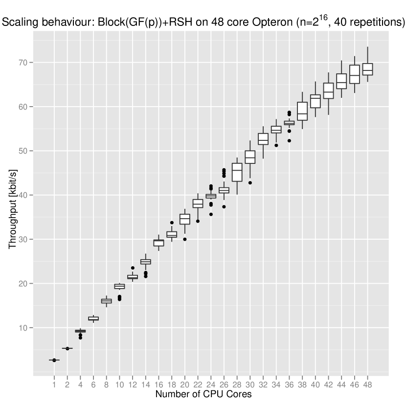
Figure 15: Throughput scaling of the block($\operatorname{GF}(p)$/RSH primitive combination for an increasing amount of CPUs. The speedup is well below one even for a moderate number of involved cores, and sees a further slow-down in the many-core case. Nonetheless, data rates that are reasonable for practical application are obtained, making the primitive combination a viable choice to post-process the output of slow devices for which it is important to not sacrifice valuable entropy, as is the case for the faster XOR extractor. While the per-core measurement in Figure 14 is more interesting from a scalability point of view, this figure provides guidance to what ressources are necessary to satisfy given experimental constraints.

Summary

We have presented a modular, scaleable implementation of Trevisan’s construction for randomness extraction, together with detailled parameter derivations and improved mathematical proofs. We have shown that the feasibility or non-feasibility of Trevisan’s scheme is not mainly a question of computational complexity issues, but does depend on the particular choice of primitives used as components of the algorithm; different scenarios require different constituents. Although our measurements indicate that there exist use cases that require theoretical improvements to make Trevisan’s construction applicable (mostly because short-seed extractors all suffer from a low extraction rate), the implementation can, for instance, satisfy the needs of all current quantum key distribution schemes. The authors hope that the public availability of the source code, together with the extensible architecture, will spawn contributions from other researchers to turn future theoretical progress into practical results.

Appendix A Extractor definitions

An extractor $\operatorname{Ext}:\{0,1\}^{n}\times\{0,1\}^{d}\to\{0,1\}^{m}$ is a function which takes a weak source of randomness $X$ and a uniformly random, short seed $Y$, and produces some output $\operatorname{Ext}(X,Y)$, which is almost uniform. The extractor is said to be strong, if the output is approximately independent of the seed.

The distance from uniform is measured by the trace distance, defined as $d(\rho,\sigma):=\frac{1}{2}\|\rho-\sigma\|_{\operatorname{tr}}$, where $\|\cdot\|_{\operatorname{tr}}$ denotes the trace norm given by $\|A\|_{\operatorname{tr}}:=\operatorname{tr}\sqrt{A^{\dagger}A}$.

Definition A.1 (strong extractor Nisan and Zuckerman (1996)).

A function $\operatorname{Ext}:\{0,1\}^{n}\times\{0,1\}^{d}\to\{0,1\}^{m}$ is a $(k,\varepsilon)$-strong extractor, if for all distributions $X$ with min-entropy $H_{\min}(X)\geq k$ and a uniform seed $Y$, we have

$$\frac{1}{2}\|\rho_{\operatorname{Ext}(X,Y)Y}-\tau_{U}\otimes\rho_{Y}\|_{\operatorname{tr}}\leq\varepsilon,$$

where $\tau_{U}$ is the fully mixed state on a system of dimension $2^{m}$.

When (quantum) side information $E$ about the source $X$ is present, the randomness of the source is measured relative to this side information. We also require the output of the extractor to be close to uniform and independent from $E$.

Definition A.2 (quantum/proof strong extractor (König and Renner, 2011, Section 2.6)).

A function $\operatorname{Ext}:\{0,1\}^{n}\times\{0,1\}^{d}\to\{0,1\}^{m}$ is a quantum/proof (or simply quantum) $(k,\varepsilon)$-strong extractor, if for all states $\rho_{XE}$ classical on $X$ with $H_{\min}(X|E)_{\rho}\geq k$, and for a uniform seed $Y$, we have

$$\frac{1}{2}\|\rho_{\operatorname{Ext}(X,Y)YE}-\tau_{U}\otimes\rho_{Y}\otimes\rho_{E}\|_{\operatorname{tr}}\leq\varepsilon,$$

where $\tau_{U}$ is the fully mixed state on a system of dimension $2^{m}$.

The function $\operatorname{Ext}$ is a classical/proof $(k,\varepsilon)$-strong extractor with uniform seed if the same holds with the system $E$ restricted to classical states.

Note that any conventional extractor (Definition A.1) is classical/proof with slightly weaker parameters.

Lemma A.3 ((König and Renner, 2011, Section 2.5),(König and Terhal, 2008, Proposition 1)).

Any $(k,\varepsilon)$-strong extractor is a classical/proof $(k+\log 1/\varepsilon,2\varepsilon)$-strong extractor.

In the extractor constructions described in Section III, we are particularly interested in extractors which only need to process a few bits of the input for every bit of output. These extractors are called local, and defined as follows.

Definition A.4 ($\ell$-local extractor Vadhan (2004)).

An extractor $\operatorname{Ext}:\{0,1\}^{n}\times\{0,1\}^{d}\to\{0,1\}^{m}$ is $\ell$-locally computable (or $\ell$-local), if for every $y\in\{0,1\}^{d}$, the function $x\mapsto\operatorname{Ext}(x,y)$ depends on only $\ell$ bits of its input, where the bit locations are determined by $y$.

This notion of local extractors applies equally to extractors with and without (quantum) side information.

Appendix B Known extractor results

The next sections contain many known theorems on extractors, which we need to derive the parameters of the constructions from Section III.

B.1 List-decodable codes

A standard error correcting code guarantees that if the error is small, any string can be uniquely decoded. A list-decodable code guarantees that for a larger (but bounded) error, any string can be decoded to a list of possible messages.

Definition B.1 (list-decodable code Sudan (2000)).

A code $C:\{0,1\}^{n}\to\{0,1\}^{\bar{n}}$ is said to be $(\varepsilon,L)$-list-decodable if every Hamming ball of relative radius $1/2-\varepsilon$ in $\{0,1\}^{\bar{n}}$ contains at most $L$ codewords.

List-decodable error correcting codes are known to be $1$-bit extractors Lu (2004); Vadhan (2004). This has been rewritten out explicitly in De et al. (2012).

Lemma B.2 ((De et al., 2012, Theorem D.3)).

Let $C:\{0,1\}^{n}\to\{0,1\}^{\bar{n}}$ be an $(\varepsilon,L)$-list-decodable code. Then the function

$$C^{\prime}:\{0,1\}^{n}\times[\bar{n}] \to\{0,1\}$$

$$(x,y) \mapsto C(x)_{y},$$

is a $(\log L+\log\frac{1}{2\varepsilon},2\varepsilon)$-strong extractor.

As noted in a footnote of De et al. (2012), this lemma can be strengthened to classical/proof extractors.

Lemma B.3.

Let $C:\{0,1\}^{n}\to\{0,1\}^{\bar{n}}$ be an $(\varepsilon,L)$-list-decodable code. Then the function

$$C^{\prime}:\{0,1\}^{n}\times[\bar{n}] \to\{0,1\}$$

$$(x,y) \mapsto C(x)_{y},$$

is a classical/proof $(\log L+\log\frac{1}{2\varepsilon},2\varepsilon)$-strong extractor.

B.2 One-bit extractors

König and Terhal König and Terhal (2008) show that any one-bit extractor is quantum/proof.

Theorem B.4 ((König and Terhal, 2008, Theorem III.1)).

Let $C:\{0,1\}^{n}\times\{0,1\}^{t}\to\{0,1\}$ be a $(k,\varepsilon)$-strong extractor. Then $C$ is a quantum/proof $(k+\log 1/\varepsilon,3\sqrt{\varepsilon})$-strong extractor.

If we however have a construction which has already been shown to be a classical/proof $(k,\varepsilon)$-strong extractor, then Theorem B.4 can be refined as follows.

Lemma B.5 (Implicit in König and Terhal (2008)).

Let $C:\{0,1\}^{n}\times\{0,1\}^{t}\to\{0,1\}$ be a classical/proof $(k,\varepsilon)$-strong extractor. Then $C$ is a quantum/proof $(k,(1+\sqrt{2})\sqrt{\varepsilon})$-strong extractor.

B.3 Universal hashing

A family of hash functions is almost universal, if the probability of a collision is low.

Definition B.6 (Stinson (1994)).

A family of hash functions $\{h:\mathcal{X}\to\mathcal{Z}\}$ is said to be $\delta$-almost universal₂ ($\delta$-AU₂), if for any $x,x^{\prime}\in\mathcal{X}$ with $x\neq x^{\prime}$,

$$\Pr_{h}\mathopen{}\mathclose{{}\left[h(x)=h(x^{\prime})}\right]\leq\delta,$$

where the hash functions are chosen uniformly at random.

The family is said to be universal₂, if it is $\delta$-AU₂ with $\delta=\frac{1}{|\mathcal{Z}|}$.

Tomamichel et al. Tomamichel et al. (2011) show that for such a family of hash functions $\{h_{y}\}_{y}$, the corresponding extractor – defined as $\operatorname{Ext}(x,y):=h_{y}(x)$ – is quantum/proof if $\delta$ is small enough.

Theorem B.7 ((Tomamichel et al., 2011, Theorem 7)).

If a family of hash functions $\mathopen{}\mathclose{{}\left\{h:\{0,1\}^{n}\to\{0,1\}^{m}}\right\}$ is $\delta$-AU₂ for $\delta=\frac{1+2\varepsilon^{2}}{2^{m}}$, then chosen uniformly at random, they build a quantum/proof $(m+4\log\frac{1}{\varepsilon}+1,2\varepsilon)$-strong extractor.

B.4 Trevisan’s extractor

In (De et al., 2012, Theorem 4.6), De et al. show that if a $(k,\varepsilon)$-strong one-bit extractor is used in Trevisan’s construction, the final extractor is a quantum/proof $(k+rm+\log 1/\varepsilon,3m\sqrt{\varepsilon})$-strong extractor, where $m$ is the output length and $r$ is a parameter of the weak design.

That theorem is the combination of the following implicit lemma and Lemma A.3.

Lemma B.8 (Implicit in De et al. (2012)).

Let $C:\{0,1\}^{n}\times\{0,1\}^{t}\to\{0,1\}$ be a quantum/proof $(k,\varepsilon)$-strong extractor with uniform seed and $S_{1},\dotsc,S_{m}\subset[d]$ a weak $(m,t,r,d)$-design. Then Trevisan’s extractor, $\operatorname{Ext}_{C}:\{0,1\}^{n}\times\{0,1\}^{d}\to\{0,1\}^{m}$, is a quantum/proof $(k+rm,m\varepsilon)$-strong extractor.

If we use a one-bit extractor which is known to be quantum proof, we get better parameters from Lemma B.8 than (De et al., 2012, Theorem 4.6).

Appendix C Weak design proofs

C.1 Basic construction

Lemma C.1.

The weak design construction described in Section III.2.1 has $r<2e$.

Proof.

Ma and Tan Ma and Tan (2011) prove that if $m\in[t^{c},t^{c+1}]$ and $t^{c}$ divides $m$, then the weak design has $r<e$. The lemma is thus immediate for $m=kt^{c}$ and any integer $1\leq k\leq t$.

Let $kt^{c}<m<(k+1)t^{c}$ for some integer $1\leq k<t$. Since the construction for $m$ is the same as the construction for $m^{\prime}=(k+1)t^{c}$ with the last sets $S_{p}$ dropped, the overlap can only decrease. Thus

$$\sum_{q<p}2^{|S_{q}\cap S_{p}|}<em^{\prime}=\frac{(k+1)e}{k}kt^{c}<\frac{k+1}{k}em\leq 2em.\qed$$

C.2 Reducing the overlap

Lemma C.2.

The weak design construction described in Section III.2.2 has $r=1$.

Proof.

For simplicity, we number the sets of the weak design $W$ with two indices $(i,j)$, where $0\leq i\leq\ell$ and $1\leq j\leq m_{i}$, and label the corresponding set of the basic weak design $S^{i}_{j}$. We need to show that the second condition of Definition III.1 holds for $r=1$, namely that for all $(i,j)$,

$$\sum_{(g,h)<(i,j)}2^{|S_{g,h}\cap S_{i,j}|}\leq m,$$

where $\{(g,h):(g,h)<(i,j)\}:=\bigcup_{g<i}\{(g,h):h\leq m_{g}\}\cup\{(i,h):h<j\}$.

Note that (4) implies that for all $0\leq k\leq\ell-1$,

$$\sum_{j\leq k}n_{j}\leq\sum_{j\leq k}m_{j}<\sum_{j\leq k}n_{j}+1,$$ (7)

from which we get

$$m_{k}<\sum_{j\leq k}n_{j}-\sum_{j\leq k-1}m_{j}+1\leq n_{k}+1.$$ (8)

Furthermore, from the sum of a geometric series, we have

$$\sum_{j\leq k-1}n_{j}+r^{\prime}n_{k} =\frac{1-\mathopen{}\mathclose{{}\left(1-\frac{1}{r^{\prime}}}\right)^{k}}{1-\mathopen{}\mathclose{{}\left(1-\frac{1}{r^{\prime}}}\right)}n_{0}+r^{\prime}\mathopen{}\mathclose{{}\left(1-\frac{1}{r^{\prime}}}\right)^{k}n_{0}$$

$$=r^{\prime}n_{0}=m-r^{\prime}.$$ (9)

For any two sets $S_{i,j}$ and $S_{g,h}$ with $i\neq g$, we have $|S_{g,h}\cap S_{i,j}|=0$. Thus for any set $S_{i,j}$ with $i\leq\ell-1$, we have

$$\sum_{(g,h)<(i,j)}2^{|S_{g,h}\cap S_{i,j}|} =\sum_{g<i,h\leq m_{g}}1+\sum_{h<j}2^{|S^{i}_{h}\cap S^{i}_{j}|}$$

$$\leq\sum_{g<i}m_{g}+r^{\prime}m_{i}$$

$$<\sum_{g<i}n_{g}+1+r^{\prime}(n_{i}+1)$$

$$=m+1,$$

where we used (7) and (8) in the second from the last line, and (9) in the last line. Since the LHS of the above inequality is an integer, and the inequality is strict, we must have

$$\sum_{(g,h)<(i,j)}2^{|S_{g,h}\cap S_{i,j}|}\leq m.$$

Finally, for the case of $S_{\ell,j}$, note that $\ell$ was chosen such that $m_{\ell}\leq t$. This can be seen as follows.

$$m_{\ell} =m-\sum_{j\leq\ell-1}m_{j}\leq m-\sum_{j\leq\ell-1}n_{j}$$

$$=m-\frac{1-\mathopen{}\mathclose{{}\left(1-\frac{1}{r^{\prime}}}\right)^{\ell}}{1-\mathopen{}\mathclose{{}\left(1-\frac{1}{r^{\prime}}}\right)}\mathopen{}\mathclose{{}\left(\frac{m}{r^{\prime}}-1}\right)$$

$$=r^{\prime}+\mathopen{}\mathclose{{}\left(1-\frac{1}{r^{\prime}}}\right)^{\ell}\mathopen{}\mathclose{{}\left(m-r^{\prime}}\right).$$

By plugging (3) in this, we get $m_{\ell}\leq t$. Since $t$ is the size of the finite field, the polynomial used to generate the elements of $S_{\ell,j}$ has all coefficients $0$, except the constant term which is $j$. We thus have $S^{\ell}_{j}=\{(x,j)\}_{x\in\operatorname{GF}(t)}$, and so the sets $\{S_{\ell,j}\}_{j\in\operatorname{GF}(t)}$ have no intersection. Hence

$$\sum_{(g,h)<(\ell,j)}2^{|S_{g,h}\cap S_{\ell,j}|}\leq\sum_{g\leq\ell}m_{\ell}=m.\qed$$

References

- Bosley and Dodis (2007) Carl Bosley and Yevgeniy Dodis, “Does privacy require true randomness?” in Theory of Cryptography, Lecture Notes in Computer Science, Vol. 4392, edited by Salil Vadhan (Springer, 2007) pp. 1–20.
- Shaltiel (2002) R Shaltiel, “Recent developments in explicit constructions of extractors,” Bulletin of the EATCS 77, 67–95 (2002).
- Trevisan (2001) Luca Trevisan, “Extractors and pseudorandom generators,” Journal of the ACM 48, 860–879 (2001).
- De et al. (2012) Anindya De, Christopher Portmann, Thomas Vidick, and Renato Renner, “Trevisan’s extractor in the presence of quantum side information,” SIAM Journal on Computing 41, 915–940 (2012), http://arxiv.org/abs/0912.5514 arXiv:0912.5514 .
- Renner (2005) Renato Renner, Security of Quantum Key Distribution, Ph.D. thesis, Swiss Federal Institute of Technology Zurich (2005), http://arxiv.org/abs/quant-ph/0512258 quant-ph/0512258 .
- Tomamichel et al. (2011) Marco Tomamichel, Christian Schaffner, Adam Smith, and Renato Renner, “Leftover hashing against quantum side information,” in IEEE Trans. Inf. Theory, Vol. 57 (8) (IEEE, 2011) pp. 5524–5535, http://arxiv.org/abs/arXiv:1002.2436 arXiv:1002.2436 .
- Ma et al. (2012) X. Ma, F. Xu, H. Xu, X. Tan, B. Qi, and H.-K. Lo, “Postprocessing for quantum random number generators: entropy evaluation and randomness extraction,” (2012), http://arxiv.org/abs/1207.1473 arXiv:1207.1473 .
- Gavinsky et al. (2008) Dmitry Gavinsky, Julia Kempe, Iordanis Kerenidis, Ran Raz, and Ronald de Wolf, “Exponential separation for one-way quantum communication complexity, with applications to cryptography,” SIAM J. Comput. 38, 1695–1708 (2008).
- Radhakrishnan and Ta-Shma (2000) Jaikumar Radhakrishnan and Amnon Ta-Shma, “Bounds for dispersers, extractors, and depth-two superconcentrators,” SIAM Journal on Discrete Mathematics 13, 2–24 (2000).
- Håstad et al. (1999) J. Håstad, R. Impagliazzo, L. Levin, and M. Luby, “A pseudorandom generator from any one-way function,” SIAM Journal on Computing 28, 1364–1396 (1999).
- Mauerer (2008) Wolfgang Mauerer, Professional Linux Kernel Architecture (Wrox, 2008).
- of Standards and Technology (2002) National Institute of Standards and Technology, FIPS 180-2, Secure Hash Standard, Federal Information Processing Standard (FIPS), Publication 180-2, Tech. Rep. (Department of commerce, 2002).
- Vadhan (2007) Salil Vadhan, “The unified theory of pseudorandomness: guest column,” SIGACT News 38 (2007).
- Nisan and Wigderson (1994a) Noam Nisan and Avi Wigderson, “Hardness vs. randomness,” Journal of Computer and System Sciences 49, 149–167 (1994a).
- Raz et al. (2002) Ran Raz, Omer Reingold, and Salil Vadhan, “Extracting all the Randomness and Reducing the Error in Trevisan’s Extractors,” Journal of Computer and System Sciences 65, 97–128 (2002).
- Hartman and Raz (2003) Tzvika Hartman and Ran Raz, “On the distribution of the number of roots of polynomials and explicit weak designs,” Random Structures and Algorithms 23, 235–263 (2003).
- Nisan and Wigderson (1994b) Noam Nisan and Avi Wigderson, “Hardness vs randomness,” Journal of Computer and System Sciences 49, 149–167 (1994b).
- Ma and Tan (2011) Xiongfeng Ma and Xiaoqing Tan, An explicit combinatorial design, Tech. Rep. (2011) eprint, http://arxiv.org/abs/arXiv:1109.6147 arXiv:1109.6147 .
- Impagliazzo et al. (2009) Russell Impagliazzo, Ragesh Jaiswal, and Valentine Kabanets, “Approximate list-decoding of direct product codes and uniform hardness amplification,” SIAM Journal on Computing 39, 564–605 (2009).
- Lu (2004) Chi-Jen Lu, “Encryption against Storage-Bounded Adversaries from On-Line Strong Extractors,” Journal of Cryptology 17, 27–42 (2004).
- Vadhan (2004) Salil P. Vadhan, “Constructing locally computable extractors and cryptosystems in the bounded-storage model,” Journal of Cryptology 17, 43–77 (2004).
- Goldreich (2011) Oded Goldreich, Studies in Complexity and Cryptography, edited by Oded Goldreich, Lecture Notes in Computer Science, Vol. 6650 (Springer Berlin Heidelberg, Berlin, Heidelberg, 2011) pp. 451–464.
- Hoory et al. (2006) Shlomo Hoory, Nathan Linial, and Avi Wigderson, “Expander graphs and their applications,” American Mathematical Society. Bulletin. New Series 43, 439–561 (2006).
- Stinson (1995) Douglas R. Stinson, “On the connections between universal hashing, combinatorial designs and error-correcting codes,” Electronic Colloquium on Computational Complexity (ECCC) 2 (1995).
- Stinson (1994) Douglas R. Stinson, “Universal hashing and authentication codes,” Designs, Codes and Cryptography 4, 369–380 (1994), a preliminary version appeared at CRYPTO ’91.
- Stroustrup (2000) Bjarne Stroustrup, The C++ Programming Language: Special Edition, 3rd ed. (Addison-Wesley Professional, 2000).
- Shoup (2005) Victor Shoup, A Computational Introduction to Number Theory and Algebra (Cambridge University Press, 2005).
- OpenSSL Project (2003) The OpenSSL Project, “OpenSSL: The open source toolkit for SSL/TLS,” (2003).
- Reinders (2007) James Reinders, Intel Threading Building Blocks: Outfitting C++ for Multi-Core Processor Parallelism, 1st ed. (O’Reilly Media, 2007).
- Herlihy and Shavit (2008) Maurice Herlihy and Nir Shavit, The Art of Multiprocessor Programming, 1st ed. (Morgan Kaufmann, 2008).
- Eddelbuettel and Francois (2012) Dirk Eddelbuettel and Romain Francois, RInside: C++ classes to embed R in C++ applications (2012), r package version 0.2.8.
- R Development Core Team (2011) R Development Core Team, R: A Language and Environment for Statistical Computing, R Foundation for Statistical Computing, Vienna, Austria (2011), ISBN 3-900051-07-0.
- Golub and van Loan (1996) Gene H. Golub and Charles F. van Loan, Matrix Computations (Johns Hopkins Studies in Mathematical Sciences)(3rd Edition), 3rd ed. (The Johns Hopkins University Press, 1996).
- Arndt (2010) Jörg Arndt, Matters Computational (Springer Berlin / Heidelberg, 2010).
- Knuth (1997) Donald E. Knuth, Art of Computer Programming, Volume 2: Seminumerical Algorithms, 3rd ed. (Addison-Wesley Professional, 1997).
- Gabriel et al. (2010) Christian Gabriel, Christoffer Wittmann, Denis Sych, Ruifang Dong, Wolfgang Mauerer, Ulrik L. Andersen, Christoph Marquardt, and Gerd Leuchs, “A generator for unique quantum random numbers based on vacuum states,” Nature Photonics 4, 711–715 (2010).
- Nisan and Zuckerman (1996) Noam Nisan and David Zuckerman, “Randomness is linear in space,” Journal of Computer and System Sciences 52, 43–52 (1996), a preliminary version appeared at STOC ’93.
- König and Renner (2011) Robert König and Renato Renner, “Sampling of min-entropy relative to quantum knowledge,” IEEE Transactions on Information Theory 57, 4760–4787 (2011), http://arxiv.org/abs/arXiv:0712.4291 arXiv:0712.4291 .
- König and Terhal (2008) Robert König and Barbara M. Terhal, “The bounded-storage model in the presence of a quantum adversary,” IEEE Transactions on Information Theory 54, 749–762 (2008), http://arxiv.org/abs/arXiv:quant-ph/0608101 arXiv:quant-ph/0608101 .
- Sudan (2000) Madhu Sudan, “List decoding: algorithms and applications,” SIGACT News 31, 16–27 (2000).