The 21-cm signature of the first stars during the Lyman-Werner feedback era

Abstract

The formation of the first stars is an exciting frontier area in astronomy. Early redshifts ($z\sim 20$) have become observationally promising as a result of a recently recognized effect (, 2010) of a supersonic relative velocity between the dark matter and gas. This effect produces prominent structure on 100 comoving Mpc scales, which makes it much more feasible to detect 21-cm fluctuations from the epoch of first heating (Visbal et al., 2012). We use semi-numerical hybrid methods to follow for the first time the joint evolution of the X-ray and Lyman-Werner radiative backgrounds, including the effect of the supersonic streaming velocity on the cosmic distribution of stars. We incorporate self-consistently the negative feedback on star formation induced by the Lyman-Werner radiation, which dissociates molecular hydrogen and thus suppresses gas cooling. We find that the feedback delays the X-ray heating transition by a $\Delta z\sim 2$, but leaves a promisingly large fluctuation signal over a broad redshift range. The large-scale power spectrum is predicted to reach a maximal signal-to-noise ratio of S/N$\sim 3-4$ at $z\sim 18$ (for a projected first-generation instrument), with S/N$>1$ out to $z\sim 22-23$. We hope to stimulate additional numerical simulations as well as observational efforts focused on the epoch prior to cosmic reionization.

1 Introduction

Observations of the redshifted 21-cm line of neutral hydrogen, planned for the next decade, are expected to usher in a new era of direct probing of the epoch of first stars. Though currently the main observational focus is on the reionization epoch, there are instruments hoping to observe the 21-cm signal from $z\sim 10-30$, e.g., LEDA (Burns et al., 2011), DARE, and the SKA (Carilli et al., 2004).

The formation of the first stars is a relatively clean theoretical problem, as they are formed in a metal-free environment via H₂ cooling (Tegmark et al., 1997; Machacek et al., 2001; Abel et al., 2002). The radiation produced by these first radiant objects changed the cosmic landscape dramatically (Madau, 1997). Three wavelength regimes of this radiation are most important to consider: the Lyman-$\alpha$ photons couple to the 21-cm line at high redshifts ($z\sim 30$) through the Wouthuysen-Field effect (Wouthuysen, 1952; , 1959); X-ray photons, produced by stellar remnants, heat the gas; and Lyman-Werner (LW) photons dissociate molecular hydrogen, thus producing negative feedback on star formation (Haiman et al., 1997) and decreasing the heating rate.

The radiation spreads out to $\sim 100$ Mpc around each star, where this finite effective horizon arises from redshift, time delay and optical depth effects (, 2009; Mesinger et al., 2011; Holzbauer & Furlanetto, 2011; Visbal et al., 2012). As star formation progresses, the radiative backgrounds build up. Fluctuations in the radiative backgrounds (Barkana & Loeb, 2005; Pritchard & Furlanetto, 2006), caused by the strongly fluctuating distribution of stars (Barkana & Loeb, 2004), couple to the hyperfine transition of neutral hydrogen and imprint fluctuations in the redshifted 21-cm signal. Whereas Lyman-$\alpha$ coupling saturates at high redshifts (Holzbauer & Furlanetto, 2011; Visbal et al., 2012), the heating fluctuations couple to the 21-cm brightness temperature at lower redshifts and thus are more interesting in terms of the observational prospects. In particular, Visbal et al. (2012) predict detectible heating fluctuations from the first stars at $z=20$ with a distinctive signature of Baryon Acoustic Oscillations (BAOs) imprinted by the supersonic relative (streaming) velocity between the baryons and the dark matter (, 2010; Dalal, Pen & Seljak, 2010).

In this paper we study the signature of the heating fluctuations including the affect of relative velocity as in Visbal et al. (2012), and add for the first time a detailed three-dimensional calculation of the inhomogeneous negative feedback by LW photons. We use the same semi-numerical hybrid methods as in Visbal et al. (2012) (based in part on (2010) and Mesinger et al. (2011)) to build a simulation where the stellar population and the radiative backgrounds evolve simultaneously in time. The basic idea is to linearly evolve a realistic sample of the Universe on large scales while using the results of numerical simulations and analytical models to add in the stars. For a detailed discussion of our computational methods, we refer the interested reader to Visbal et al. (2012), in particular to section S1 of this paper’s Supplementary Information, and references within. We use the standard set of cosmological parameters (Komatsu et al., 2010) along with an assumed star formation efficiency (fraction of gas in star-forming halos that turns to stars) of $f_{*}=10\%$, an X-ray photon efficiency of $10^{57}M_{\odot}^{-1}$ based on observed starbursts at low redshift as in Mesinger et al. (2011), and LW parameters as explained in the next section.

2 Incorporating the Negative Feedback

The formation of the first stars via cooling of molecular hydrogen is a highly non-linear process that can be mimicked by numerical simulations, e.g., Abel et al. (2002); Bromm et al. (2002). However, numerical simulations in which primordial stars are created usually do not consider the potentially fatal effect of the LW background on this process. The negative feedback of the LW background on star formation has been tested in the limited case of a fixed intensity $J_{{\rm LW}}$ (Machacek et al., 2001; Wise & Abel, 2007; O’Shea & Norman, 2008). The feedback boosts the minimal cooling mass, $M_{\rm cool}$, i.e., the mass of the lightest halo in which stars can form, with the results of these simulations well-described by the relation

$$M_{\rm cool}\left(J_{21},z\right)=M_{{\rm cool},0}(z)\times\left[1+6.96\left(4\pi J_{21}\right)^{0.47}\right],$$ (1)

where $J_{21}=J_{{\rm LW}}/(10^{-21}$erg s^-1cm^-2Hz^-1sr${}^{-1})$ in terms of the LW intensity $J_{{\rm LW}}$; another common notation is the LW flux $F_{{\rm LW}}=4\pi J_{{\rm LW}}$. Here $M_{{\rm cool},0}(z)$ is the value of the minimum cooling mass in the standard case with no LW background.

This result is incomplete for two reasons. One is that it does not account for the relative velocity $v_{\rm bc}$, which has a strong impact on the primordial star formation by (among other things) boosting the minimum cooling mass (, 2011; Stacy et al., 2011; , 2011). To account for the velocity, we change $M_{{\rm cool},0}(z)$ in Eq. (1) to $M_{{\rm cool},0}(z,v_{\rm bc})$, using the fit we developed in (2011) to the streaming-velocity simulations (here we use their fit designed for Adaptive Mesh Refinement (AMR) simulations as equation (1) was the result of a fit to an AMR simulation). Thus, we combine two separate physical phenomena, i.e., the relative motion and the LW flux, assuming that they each have a fixed multiplicative effect on the minimum cooling mass. This simple ansatz for the dependence of $M_{{\rm cool}}$ on the two parameters, $v_{\rm bc}$ and $J_{21}$, should be checked by detailed numerical simulation, which we hope to stimulate with this work. We choose this multiplicative ansatz since both effects have an independent effect on the minimal cooling mass. Therefore they likely reinforce each other when they are both present. We note that while we include the $v_{\rm bc}$ and LW effects separately in Eq. (1), our results do account for the strong correlation between the velocity and the LW flux (due to the effect of the velocity on star formation).

The second incompleteness of Eq. (1) is its validity only in the case of a fixed background intensity during the formation of the halo, whereas in reality the LW intensity is expected to rise exponentially with time at high redshifts (e.g., see the Supplementary Information in Visbal et al. (2012)). Treating the intensity as fixed at its final value would greatly overestimate the strength of the feedback, since the cooling and collapse involved in star formation should respond with a delay to a drop in the amount of H₂. For instance, if the halo core has already cooled and is collapsing to a star, changing the LW flux may not stop or reverse the collapse at all, and certainly not immediately. Another indication for the gradual process involved is that the simulation results can be approximately matched (Machacek et al., 2001) by comparing the cooling time in halo cores to the Hubble time (which is a relatively long timescale). Though the relation in Eq. (1) is the best currently available, more elaborate numerical simulations, which we again hope to stimulate, are needed in order to find a more realistic dependence. We overcome this limitation by using the above relation not with the final value of $J_{21}$ at formation, but with the value at a mean, characteristic time within the halo formation process.

The idea of looking at the flux at times well before virialization is based on an analogy with the filtering mass defined in the well-studied case of pressure (, 1998; Gnedin, 2000). In the latter case, the actual gas fraction in non-linear, virialized halos, is close to the filtering mass, not the Jeans mass, and the filtering mass is affected by the value of the Jeans mass at much earlier times. The reason the gas fraction is affected by the Jeans mass at early times is that the relationship between the gas temperature and the gas density is very indirect; the temperature affects the pressure gradient, and thus the acceleration, which affects the actual position after a delay. In particular, if the temperature drops suddenly, the gas that was far away from the halo center does not instantly fall inside. In the case of cooling, there are the additional steps from dissociation of H₂, which changes its abundance, through the process of cooling which then affects the temperature. The cooling history thus affects the distribution of gas. The LW flux rises exponentially fast with time and was very small at early times. Thus, the cooling was fast initially, and the gas cooled and started to collapse. A sudden late rise in the flux may not be able to stop this collapse.

Using the characteristic value of $J_{21}$ with a realistically large uncertainty should suffice for our main goal of spanning the possible range of the effect of $J_{{\rm LW}}$ and $v_{\rm bc}$ on the 21-cm background during the X-ray heating era. Specifically, we consider two possible feedback strengths which we refer to as “weak” and “strong” feedback. Namely, for halos forming (i.e., virializing) at some time $t_{\rm vir}$, we adopt the effective LW flux $J_{21}$ in Eq. (1) as the LW flux in the same pixel at an earlier time $t_{\rm mid}$, i.e., at the midpoint of the halo formation process. In order to obtain a realistically large range of uncertainty, with the spherical collapse model in mind we either assume that “formation” spans the beginning of expansion up to virialization (i.e., $t=0$ to $t=t_{\rm vir}$, giving $t_{\rm mid}=\frac{1}{2}t_{\rm vir}$: weak feedback), or just the collapse stage starting at turnaround (i.e., $t=\frac{1}{2}t_{\rm vir}$ to $t=t_{\rm vir}$, giving $t_{\rm mid}=\frac{3}{4}t_{\rm vir}$: strong feedback). We also compare to the limiting cases (shown in Visbal et al. (2012)) of no feedback or saturated feedback. The latter correponds to assuming that star formation is only possible via atomic cooling; in this scenario, the LW feedback is so efficient that H₂ is completely dissociated early on and stars form in atomic cooling halos ($M_{{\rm cool}}\ga 3\times 10^{7}M_{\odot}$), as opposed to $M_{{\rm cool}}\la 10^{6}M_{\odot}$. For reference, we also consider the no feedback case without the streaming velocity, in order to assess the importance of the velocity effect. For given parameters, at each redshift the cosmic mean gas fraction in stars decreases in the different cases in the order: no feedback no velocity, no feedback, weak feedback, strong feedback, and saturated feedback (where all cases except the first include the streaming velocity effect).

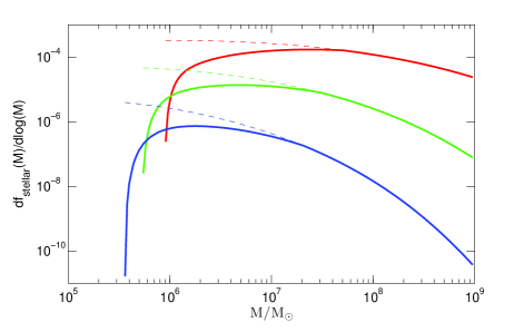
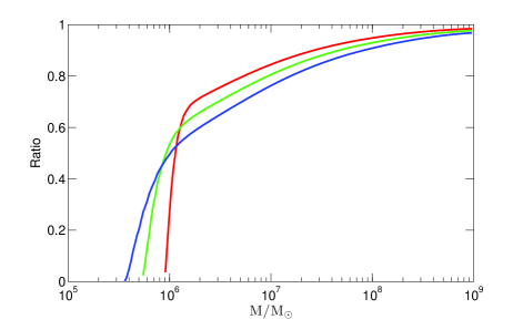
Figure 1: Star-formation contribution and effect of velocities versus halo mass (LW feedback not included). Left: The logarithmic contribution of each halo mass to the total fraction of gas in stars (i.e., $df_{\rm stellar}/d\log(M)$ averaged over the distribution of $v_{\rm bc}$), including the $\log(M)$ modulation in Equation (2) (solid) or with the standard assumption of a fixed efficiency with mass (dashed). We consider $z=13.6$ (red), $z=19.6$ (green), and $z=25.6$ (blue). Right: The ratio of the cosmic mean stellar fraction with $v_{\rm bc}$ to the value without the velocity effect, i.e., $<f_{\rm stellar}(M,v_{\rm bc})>_{v_{\rm bc}}/f_{\rm stellar}(M,0)$. We include Equation (2), and consider the same redshifts as in the left panel.

In our hybrid simulations we also incorporate two elements of the astrophysics that make our calculations more complete and accurate. One aspect is that we include a gradual low-mass cutoff for star formation, rather than a sharp cutoff at $M_{\rm cool}$ as we (and others) have previously assumed. Since the cooling rate declines smoothly with virial temperature, a smooth cutoff is expected physically, and indeed Machacek et al. (2001) found that the fraction of highly-cooled, dense gas in their simulated halos is well described as being proportional to $\log(M/M_{\rm cool})$. Since this is the gas that can participate in star formation, we incorporate this by generalizing the star-formation efficiency to include a dependence on halo mass, $f_{*}(M)$. We assume our standard efficiency of $f_{*}=10\%$ for $M\geq M_{\rm atomic}$, where $M_{\rm atomic}$ is the minimum mass for atomic cooling ($\sim 3\times 10^{7}M_{\odot}$ but $z$-dependent). In order for $f_{*}(M)$ to be a continuous function, we thus set

$$f_{*}(M)=\left\{\begin{array}[]{ll}f_{*}&\mbox{if $M\geq M_{\rm atomic}$}\\ f_{*}\frac{\log(M/M_{\rm cool})}{\log(M_{\rm atomic}/M_{\rm cool})}&\mbox{if $M_{\rm cool}<M<M_{\rm atomic}$}\\ 0&\mbox{otherwise.}\end{array}\right.$$ (2)

As shown in Figure 1 (left panel), the standard assumption of constant $f_{*}$ makes halos with masses near $M_{\rm cool}$ dominate the cosmic star formation rate, particularly at the highest redshifts. Our more realistic model significantly reduces the overall star formation rate (by a factor of 2.0 in the example shown at $z=19.6$) and shifts the peak of the contribution to star formation to a higher mass ($8.7\times M_{\rm cool}$ at $z=19.6$). Also shown in the Figure (right panel) is the overall effect of the relative velocity $v_{\rm bc}$ broken down by mass. Since the velocity effect on halos is made up of three distinct effects, with two of them dominant (, 2011), the dependence on halo mass shows two separate regimes. Near the cooling mass (and up to a factor of $\sim 2$ above it), the velocity effect is very strong and also strongly dependent on $M$, mainly due to the boosting of the cooling mass in regions with a high $v_{\rm bc}$. At higher masses, however, the velocity effect is weaker and only changes rather slowly with halo mass, mainly due to the suppression of the halo abundance. A small but non-negligible effect remains even well above $M_{\rm atomic}$. Since the velocity effect is strongest at the low-mass end (right panel), the shifting of the star formation towards higher masses (left panel) reduces somewhat the overall influence of the supersonic streaming velocities. Since the LW feedback also affects low masses first, the $\log(M)$ modulation delays the LW feedback.

The second aspect of realistic astrophysics that we incorporate is more directly related to the LW feedback. The LW photons emitted by each source are absorbed by hydrogen atoms as soon as they redshift into one of the Lyman lines of the hydrogen atom; along the way, whenever they hit a LW line they may cause a dissociation of molecular hydrogen. Some previous papers (, 2009; Holzbauer & Furlanetto, 2011) assumed a flat stellar spectrum in the LW region and a flat absorption profile over the LW frequency range. We incorporate the expected stellar spectrum of Population III stars from Barkana & Loeb (2005) (based on Bromm et al. (2001)), which varies in the LW region typically by a few percent but up to $17\%$. More importantly, we explicitly include the full list of 76 relevant LW lines from Haiman et al. (1997). We summarize the results with $f_{\rm LW}$, the relative effectiveness of causing H₂ dissociation via stellar radiation. Specifically it is the ratio between the dissociation rate of molecular hydrogen and the naive total stellar flux (i.e., calculated without any absorption and integrated over all wavelengths), normalized to unity in the limit of zero source-absorber distance. This quantity is simply a function of source-absorber distance at each redshift under the simplifying assumption of a universe at the mean density. This assumption follows our approach for X-rays (as in 21CMFAST, Mesinger et al. (2011)), and should be sufficiently accurate since the strong bias of star-forming halos at these high redshifts implies that fluctuations in star formation (which drive the 21-cm fluctuations) are much larger than the fluctuations in the underlying density. Thus, give our assumed stellar spectrum we can pre-calculate $f_{\rm LW}$ and include this as an effective optical depth that is spherically symmetric around each source. Any such symmetric effect is easily incorporated within the numerical method of 21CMFAST which uses Fourier transforms to rapidly perform averages over spherical shells.

Figure 2 shows $f_{\rm LW}$ versus the absorber-source distance; we parametrize this distance in terms of the absorber-source scale-factor ratio $R$, since $f_{\rm LW}$ versus $R$ is independent of redshift. Beyond the max shown $R=1.054$ (which corresponds to 104 comoving Mpc at $z=20$), $f_{\rm LW}$ immediately drops by five orders of magnitude. The Figure shows that LW absorption is poorly approximated as being uniform in frequency. In reality, emission from distant sources is absorbed more weakly. For example, in one of our main examples in the following section (i.e., our strong LW feedback case including velocities), assuming a uniform spectrum and absorption profile at $z=20$ would imply that typically, an atom receives $50\%$ of its LW flux from sources out to a distance of 18.9 Mpc, $80\%$ from up to 42.2 Mpc, and $90\%$ from up to 55.8 Mpc. Our more accurate $f_{\rm LW}$ reduces these numbers to 14.4, 33.0, and 46.2 Mpc, respectively. The accurate $f_{\rm LW}$ reduces the overall LW intensity by $\sim 20\%$ (thus delaying the LW feedback), and makes it more short-range (i.e., local) and variable.

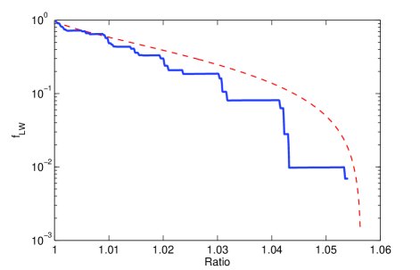
Figure 2: The relative effectiveness of causing H₂ dissociation in an absorber at $z_{a}$ due to stellar radiation from a source at $z_{s}$, shown versus the ratio $R\equiv(1+z_{s})/(1+z_{a})$ (solid). For comparison we show $f_{mod}$, a commonly used approximation from (2009) (dashed). Both functions are normalized to unity at $R=1$. (There was also a $1.45\%$ normalization difference after we carefully normalized as in Machacek et al. (2001), since we use their results for the LW feedback.)

3 Results

3.1 Mean Evolution

The relative velocity amplifies heating fluctuations in the 21-cm power spectrum, making it possible to observe the BAO in the first stars (Visbal et al., 2012; McQuinn & O’Leary, 2012). In this section we consider the effect of the negative LW feedback on this exciting observational prospect. Our simulation evolves a realistic sample of the universe from $z=60$, roughly when the first stars turn on (Naoz et al., 2006; , 2011). We follow a box that is 384 Mpc on a side (all distances comoving), with a pixel size of 3 Mpc. The X-ray and LW backgrounds in each pixel are made up of contributions by stars located within the corresponding effective horizons. Since we focus on the era after Lyman-$\alpha$ coupling but prior to significant reionization, the 21-cm brightness temperature (relative to the cosmic microwave background (CMB) temperature $T_{\rm CMB}$)Madau (1997)

$$T_{\rm b}=40(1+\delta)\left(1-\frac{T_{\rm CMB}}{T_{\rm K}}\right)\sqrt{\frac{1+z}{21}}~{}{\rm mK}\ ,$$ (3)

where $\delta$ is the gas overdensity and $T_{\rm K}$ its kinetic temperature.

The negative feedback suppresses star formation on average, which leads to a slower rise of the radiative backgrounds, and delays various milestones of the star formation history. Figure 3 shows the rise of the mean LW flux with time. Comparing the two no-feedback cases, we see that the streaming velocity has a large overall suppression effect at high redshifts, which reaches about an order of magnitude at $z>40$ but becomes quite small at $z<15$. Feedback can potentially be very strong at high redshifts (as indicated by the saturated feedback case), but in practice the LW feedback is expected to begin only when the effective flux reaches a level of $J_{21}\sim 10^{-5}$; this happens at around redshift 30 (weak feedback) or 40 (strong). In both realistic feedback cases, the LW feedback effectively saturates at $z\sim 10$.

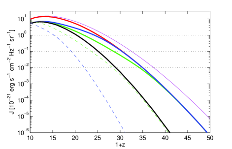
Figure 3: The actual LW intensity (solid lines) and the effective LW intensity for feedback on star formation (dashed; shown only for the two realistic feedback cases). We show the cosmic mean intensity (i.e., averaged over our box) versus $1+z$ in the following cases: no feedback no $v_{\rm bc}$ (purple), and with $v_{\rm bc}$: no feedback (red), weak feedback (blue), strong feedback (green), and saturated feedback (black).

We can easily understand why the two feedback cases converge with time. Initially, the effective LW flux for star formation [i.e., $J_{21}$ in Eq. (1)] is much higher at a given $z$ for the strong feedback case (which assumes a less delayed value, closer to the value of $J_{21}$ at $z$). The strong resulting feedback leads to a slower rise of the actual $J_{21}$ and thus, eventually, also of the effective $J_{21}$, compared to the weak feedback case. Therefore, the effective $J_{21}$ in the weak feedback case gradually catches up with the strong feedback case. Also important is that the rate of increase of the flux naturally slows with time (i.e., the curves flatten), since star-forming halos become less rare (i.e., they correspond to less extreme fluctuations in the Gaussian tail of the initial perturbations). The weak feedback case effectively looks back to $J_{21}$ at an earlier time, when the rise was faster.

Figure 3 tracks the rise of the LW flux through several milestone values. A reasonable definition of the central redshift $z_{{\rm LW}}$ of the LW transition is a mean effective intensity of $J_{21}=0.1$, at which the minimum halo mass for cooling (in the absence of streaming velocities) is raised to $\sim 2\times 10^{6}M_{\odot}$ due to the LW feedback. This is a useful fiducial mass scale, roughly intermediate (logarithmically) between the cooling masses obtained with no LW flux and with saturated LW flux. The central range of the LW feedback transition can be defined by the effective LW flux coming within an order of magnitude of its central value, so that the minimum $M_{{\rm cool}}$ goes from $8\times 10^{5}M_{\odot}$ to $5\times 10^{6}M_{\odot}$ during this period.

Feedback also slows down the heating of the Universe (Figure 4). For example, the average heating rate at redshift 20 for the weak, strong and saturated feedbacks are $55.9\%$, $33.7\%$ and $19.1\%$ of the heating rate with no feedback (all including the streaming velocity). As a result, the heating transition is delayed. There are two possible natural definitions for this transition, the standard more physical definition as the redshift $z_{\rm h}$ when the mean gas temperature equals that of the CMB, and the more observational (or 21-cm-centric) definition as the redshift (which we denote $z_{0}$) at which the cosmic mean 21-cm brightness temperature vanishes $\langle T_{\rm b}\rangle=0$. We consider both definitions, but due to our focus on observational predictions, we mostly use $z_{0}$.

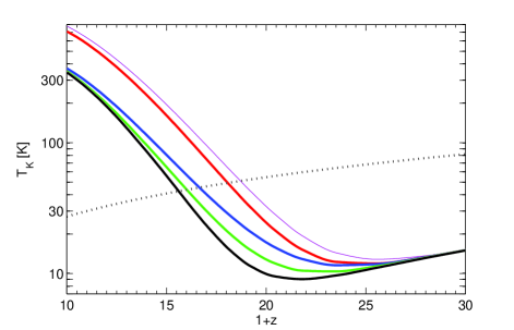
Figure 4: The cosmic heating transition. We show the cosmic mean gas kinetic temperature versus $1+z$ in the following cases: no feedback no $v_{\rm bc}$ (purple), and with $v_{\rm bc}$: no feedback (red), weak feedback (blue), strong feedback (green), and saturated feedback (black). Also shown for comparison is the CMB temperature (dotted), which crosses the gas temperature at $z_{\rm h}$.

In our simulation, $z_{\rm h}=17.1$ and $z_{0}=16.6$ for the no-feedback case (no feedback and no velocity gives $z_{\rm h}=17.7$ and $z_{0}=17.4$), while saturated feedback would delay these milestones to $z_{\rm h}=14.6$ and $z_{0}=14.2$. The realistic feedback cases are intermediate: $z_{\rm h}=15.7$ and $z_{0}=15.2$ for the weak feedback case (with a LW transition centered at $z_{\rm LW}=19.2$, and a central range of $z=22.0-15.2$), while $z_{\rm h}=15.0$ and $z_{0}=14.6$ for strong feedback (with $z_{\rm LW}=23.6$, and a central range of $z=28.3-18.1$). In every case, the LW transition starts very early, and passes through its central redshift before the heating transition (with a much bigger delay between the two transitions in the strong feedback case). We note that if all the fluctuations were linear, then we would find $z_{\rm h}=z_{0}$ identically. The difference of $\Delta z=0.4-0.5$ between them is an example of the effect of non-linear fluctuations (plus, in this case, of the non-linear dependence of the brightness temperature on the gas temperature). This shows that analyses of this era based on linear theory can only give rough estimates, and a hybrid simulation like ours is necessary in order to properly incorporate the non-linear fluctuations in stellar density and other derived quantities.

3.2 Spatial Fluctuations

The most interesting 21-cm signature of the first stars is the enhanced large-scale fluctuation level due to the supersonic streaming velocity. A typical two-dimensional slice of our simulated volume is shown in Figure 5 together with the spatial distribution of the fluctuations in the density and in the relative velocity. A snapshot of the Universe at a fixed redshift would look very distinctive in the various feedback cases mainly due to the overall delay in the heating due to the change in the mean heating rates. It is more instructive to compensate for this shift and instead compare each case to the others at the same time relative to the individual heating redshift (we use $z_{0}$).

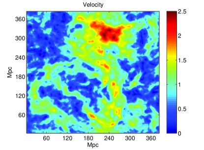
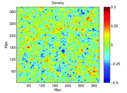
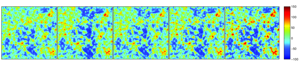
Figure 5: A two-dimensional slice of our simulated volume. All panels show the same slice, i.e., with the same initial conditions. Top: Left: The magnitude of the relative velocity between baryons and dark matter shown in units of the velocity’s root-mean-square value. Right: The relative fluctuation in density at redshift 20. Bottom: The 21-cm brightness temperature $T_{\rm b}$ (relative to the cosmic mean in each case) in mK, shown at $z_{0}+3$. The cases shown (from left to right) are: no feedback, no $v_{\rm bc}$; no feedback; weak feedback; strong feedback; and saturated feedback (where the last four include the streaming velocities). The cosmic mean values (which have been subtracted from the maps) are: $\langle T_{\rm b}\rangle=-81$ mK, -89 mK, -73 mK, -88 mK and $-108$ mK, respectively.

As seen in Figure 5, the feedback weakens the effect of the relative motion, since it boosts the minimal cooling mass so that the stars form in heavier halos which are less sensitive to the relative velocities. Thus, in Figure 5 the 21-cm signal with saturated feedback shows the same pattern as in the no $v_{\rm bc}$ case (with no feedback); namely, both of them follow the density fluctuations but with a strong enhancement, where the bias is stronger for the saturated feedback (since more massive halos are more strongly biased). The no feedback case (with $v_{\rm bc}$) shows a strong imprint of the velocity field along with the influence of density fluctuations; e.g., the enhanced $T_{\rm b}$ at the bottom right is mainly due to a density enhancement, while the void at the top (just right of center) is mainly due to a large relative velocity (but note that the 21-cm maps are the result of a three dimensional calculation of the radiation fields, so they cannot be precisely matched with two-dimensional slices of the density and velocity fields).

The two realistic feedback cases are intermediate, showing a clear velocity effect, though not as strong as in the no-feedback case. To understand the comparison between the weak and strong feedback, we note that the velocities cause a very strong suppression of star formation up to a halo mass $M\sim 10^{6}M_{\odot}$, but above this critical mass the suppression and its $M$-dependence weaken considerably (Figure 1, right panel). Thus, once the LW feedback passes through its central redshift, the remaining $v_{\rm bc}$ effect changes only slowly with $M$, so that around the time of the heating transition, the weak and strong feedback cases show a similar fluctuation pattern. However, the strong dependence of bias on $M$ remains, so that the strong feedback case leads to larger fluctuations on all scales.

These and other features can be seen more clearly and quantitatively in the power spectra (Figure 6). The 21-cm fluctuations initially rise with time as the heating becomes significant (first in the regions with a high stellar density). Eventually, as the heating spreads, the 21-cm fluctuations decline, since the 21-cm intensity becomes independent of the gas temperature once the gas is much hotter than the CMB (Equation 3). Thus, the power spectrum reaches its maximum height somewhat earlier than $z_{0}$. The comparison among the various feedback cases is complex, since the negative LW feedback has several different effects: 1) The lowest-mass halos are cut out, reducing the effect of the streaming velocity; 2) The higher-mass halos that remain are more highly biased; 3) The overall suppression of star formation delays the heating and LW transitions to lower redshifts; and 4) Since the higher-mass halos that remain correspond to rarer fluctuations in the Gaussian tail, their abundance changes more rapidly with redshift, making the heating transition more rapid (i.e., focused within a narrower redshift interval). Thus, at $z_{0}+3$ the large-scale ($k=0.05$ Mpc^-1) peak is lower for the realistic feedback cases than it would be with no feedback (due to effect #1), and higher for strong feedback than for the weak case (due to effect #2). Further back in time ($z_{0}+9$), weak feedback gives a higher large-scale peak than both strong feedback (due to effect #4) and no feedback (due to effect #2); at that redshift, saturated feedback shows no velocity effect (due to effect #4).

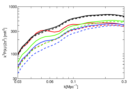
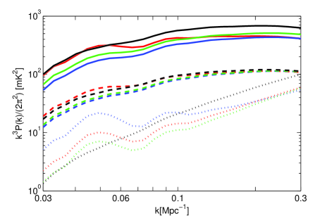
Figure 6: Power spectra of the 21-cm brightness temperature for no feedback (red), weak feedback (blue), strong feedback (green) and saturated feedback (black). Left: $z=z_{0}+3$ with (solid) or without (dashed) the relative velocity. Right: Including $v_{\rm bc}$, at redshifts $z=z_{0}$ (dashed), $z=z_{0}+3$ (solid) and $z=z_{0}+9$ (dotted).

Lower redshifts offer improved observational prospects, due to the lower foreground noise, which makes negative feedback advantageous due to effect #3, above. We find that the most promising redshift is $z\sim z_{0}+3$ (Table 1). Assuming a first-generation radio telescope array with a noise power spectrum that scales as $(1+z)^{5.2}$ (McQuinn, 2006; Visbal et al., 2012), the maximal S/N of the large-scale ($k=0.05$ Mpc^-1) peak is 3.24 for weak feedback (at $z=18.3$) and 3.91 for strong feedback (at $z=17.7$). For comparison, the no-feedback case considered in Visbal et al. (2012) gave (at $z=z_{0}=20$) a S/N of only 2.0 . It would be particularly exciting to detect the evolution of the 21-cm power spectrum throughout the heating transition, as we suggested in Visbal et al. (2012). The S/N remains above unity at all $z<z_{0}+7.9=23.1$ in the case of the weak feedback and $z<z_{0}+7.2=21.9$ for the strong feedback (down to $z=10$ where our simulations end). The streaming velocity clearly plays a key role in creating this extended observable redshift range, by boosting the large-scale power (Figure 6).

$z-z_{0}$	$\delta T_{\rm b}(k=0.05~{}{\rm Mpc}^{-1})$, S/N					BAO, S/N
	no $v_{\rm bc}$	no fbk	weak	strong	sat	no $v_{\rm bc}$	no fbk	weak	strong	sat
$-3$	1.07	1.24	1.60	1.73	1.84	0.45	0.58	0.72	0.76	0.79
$0$	1.68	2.33	2.35	2.69	3.09	0.70	1.26	1.16	1.30	1.31
$3$	2.26	3.59	3.24	3.91	4.74	0.91	2.18	1.79	2.14	2.00
$6$	1.02	1.75	2.08	1.89	1.34	0.37	1.17	1.30	1.18	0.54
$9$	0.086	0.33	0.56	0.34	0.31	0.051	0.23	0.41	0.25	0.14
$12$	0.18	0.23	0.24	0.27	0.34	0.083	0.099	0.11	0.12	0.15

Table 1: The signal to noise ratio S/N (i.e., the square root of the ratio between the power spectra of the signal and noise), for a projected first-generation radio array. We show the S/N of the large-scale peak at the wavenumber $k=0.05$ Mpc^-1 (Left), and of the BAO component (Right), at various redshifts, for five cases: no feedback no $v_{\rm bc}$. no feedback (with $v_{\rm bc}$), weak, strong and saturated feedback. The BAO S/N is defined as the square root of the difference between the peak at $k=0.05$ Mpc^-1 and the trough at $k=0.07$ Mpc^-1, each measured with respect to the non-BAO power spectrum (i.e., the power spectrum smoothed out using a quartic fit), and each normalized by the noise power spectrum at the same $k$ at the corresponding redshift.

We suggested in Visbal et al. (2012) that beyond just detecting the power spectrum, it would be particularly remarkable to detect the strong BAO signature, since this would confirm the major influence of the relative velocity and the existence of small ($10^{6}M_{\odot}$) halos. We find that the S/N for the large-scale BAO feature of the power spectrum is typically $\sim 0.5-0.7$ times that of the large-scale peak itself (Table 1). In particular, the BAO S/N also peaks at $z_{0}+3$, exceeds unity at $z_{0}-0.7<z<z_{0}+6.9$ (weak) and $z_{0}-1.1<z<z_{0}+6.4$ (strong) and reaches a maximum value of 1.79 (weak) or 2.14 (strong feedback).

We have assumed here the projected sensitivity of a thousand-hour integration time with an instrument like the Murchison Wide-field Array (Bowman et al., 2009) but designed to operate in the range of 50–100 MHz. An instrument similarly based on the Low Frequency Array (Harker et al., 2010) should improve the S/N by a factor of $\sim 1.5$, while a second-generation instrument like the SKA or a 5000-antenna MWA should improve it by at least a factor of 3 or 4 (McQuinn, 2006; Visbal et al., 2012). Thus, future instruments may be able to probe even earlier times, including the central stages of the LW feedback.

4 Conclusions

We have presented new predictions for the signature of the first stars in the heating fluctuations of the 21-cm brightness temperature. We ran hybrid simulations that allow us to predict the large-scale observable 21-cm signature while accounting on small-scales for various effects on star-formation investigated by previous analytical models and numerical simulations. In particular, we incorporated for the first time the Lyman-Werner feedback on star formation, calculated self-consistently including the effect of the supersonic streaming velocity. A three-dimensional calculation of the Lyman-Werner and X-ray backgrounds allowed us to calculate the heating history of the gas and the resulting 21-cm intensity maps.

We have focused on the negative LW feedback, which begins at $z\sim 30-40$ but strengthens very gradually, passing its central point at $z_{\rm LW}\sim 19-24$ and saturating only at $z\sim 10$. The heating transition is centered at $z_{0}\sim 15$ (including a delay of $\Delta z\sim 1.5-2$ due to the feedback), when the LW transition is well advanced but still far from saturated. The large-scale 21-cm power spectrum is potentially observable over a broad redshift range of $z\sim 10-22$ or 23. The best prospects are at $z\sim 18$, when the large-scale peak reaches a signal-to-noise ratio (for a projected first-generation radio telescope array) of 3.2 (for our weak feedback case) or 3.9 (for strong feedback). At this redshift, the BAO signature (which marks the velocity effect and the presence of $10^{6}M_{\odot}$ halos) should also be observable with a S/N$\sim 2$. The BAOs should be observable over a broad redshift range of $\Delta z\sim 7.5$ .

These numbers are obtained with our standard set of expected astrophysical parameters, but they may shift around a bit depending on the precise properties of the early stars and their remnants. We hope these findings will stimulate additional numerical simulations of the complex radiative feedback at $z\sim 10-30$, as well as future observational efforts in 21-cm cosmology directed at the epoch prior to reionization.

5 Acknowledgments

We are most grateful to Zoltan Haiman for supplying us with the atomic data on the Lyman-Werner absorption lines. This work was supported by Israel Science Foundation grant 823/09. A.F. was also supported by European Research Council grant 203247.

References

- Abel et al. (2002) Abel, T. L., Bryan, G. L., & Norman, M. L. 2002, Science 295, 93
- (2) Ahn, K., Shapiro, P. R., Iliev, I. T., Mellema, G., & Pen, U., 2009, ApJ, 695, 1430
- Barkana & Loeb (2004) Barkana R., Loeb A., 2004, ApJ, 609, 474
- Barkana & Loeb (2005) Barkana R., Loeb A., 2005, ApJ, 626, 1
- Bowman et al. (2009) Bowman J. D., Morales M. F., Hewitt J. N., 2009, ApJ, 695, 183
- Bromm et al. (2002) Bromm V., Coppi P. S., Larson R. B., 2002, ApJ, 564, 23
- Bromm et al. (2001) Bromm V., Kudritzki, R. P., & Loeb A., 2001, ApJ, 552, 464
- Burns et al. (2011) Burns, J. O., et al. 2011, AAS, ArXiv:1106.5194
- Carilli et al. (2004) Carilli, C. L., Furlanetto, S., Briggs, F., Jarvis, M., Rawlings, S., Falcke, H., 2004, NewAR, 48, 11-12
- Dalal, Pen & Seljak (2010) Dalal N., Pen U.-L., Seljak U., 2010, JCAP, 11, 7
- (11) Fialkov A., Barkana R., Tseliakhovich D., Hirata C. M. 2012, MNRAS, 424, 1335
- (12) Field G. B., 1959, ApJ, 129, 536
- Gnedin (2000) Gnedin, N. Y. 2000, ApJ, 542, 535
- (14) Gnedin N. Y., Hui L., 1998, MNRAS, 296, 44
- (15) Greif, T., White, S., Klessen, R., & Springel, V., 2011, ApJ, 736, 147
- Haiman et al. (1997) Haiman, Z., Rees, M. J., Loeb, A., 1997, ApJ, 484, 985
- Harker et al. (2010) Harker, G., 2010, MNRAS, 405, 2492
- Holzbauer & Furlanetto (2011) Holzbauer L. N., Furlanetto S. R., 2012, MNRAS, 419, 718
- Komatsu et al. (2010) Komatsu, E. et al., 2011, ApJS, 192, 18
- Machacek et al. (2001) Machacek, M. E., Bryan, G. L., Abel, T., 2001, ApJ, 548, 509
- Madau (1997) Madau, P.,Meiksin, A., Rees,M. J., 1997, ApJ, 475, 429
- McQuinn (2006) McQuinn, M., Zahn, O., Zaldarriaga, M., Hernquist, L., Furlanetto, S. R., 2006, ApJ, 653, 815
- McQuinn & O’Leary (2012) McQuinn, M., O’Leary, R., M., 2012, arXiv 1204.1334
- Mesinger et al. (2011) Mesinger, A., Furlanetto, S., Cen, R., 2011, MNRAS, 411
- Naoz et al. (2006) Naoz S., Noter S., Barkana R., 2006, MNRAS, 373, L98
- O’Shea & Norman (2008) O’Shea, B. W., Norman, M. L., ApJ, 673, 14, 2008
- Pritchard & Furlanetto (2006) Pritchard, J. R., Furlanetto, S. R., 2006, MNRAS, 367, 1057
- Stacy et al. (2011) Stacy A., Bromm V., Loeb A., 2012, MNRAS, 413, 543
- Tegmark et al. (1997) Tegmark M., Silk J., Rees M. J., Blanchard A., Abel T., Palla F., 1997, ApJ, 474, 1
- (30) Tseliakhovich D., Hirata C. M., 2010, PRD, 82, 083520
- Visbal et al. (2012) Visbal, E., Barkana, R., Fialkov, A., Tseliakhovich, D., Hirata, C. M., 2012, Nature, 487, 70
- Wise & Abel (2007) Wise, J. H., Abel, T., 2007, ApJ, 671, 1559
- Wouthuysen (1952) Wouthuysen S. A., 1952, AJ, 57, 31