Phase retrieval by power iterations

Abstract

I show that the power iteration method applied to the phase retrieval problem converges under special conditions. One is given the relative phases between small non-overlapping groups of pixels of a recorded intensity pattern, but no information on the phase between the groups of pixels. Numerical tests show that the inverse block iteration recovers the solution in 1 iteration.

I Introduction

Given a set of intensity measurements, $a^{2}\in\mathbb{R}^{M}$, an unknown object $\psi\in\mathbb{C}^{N}$ represented by a complex $n\times n$ image ($N=n^{2}$), a known “illumination matrix” or support matrix ${\bf Q}$ ($\mathbb{C}^{M\times N}$ matrix), a known propagation operator (typically one, or a stack of 2D FFT operators) $\bm{F}$ of dimension $M\times M$ and set of frames ${\bf z}\in\mathbb{C}^{M}$, which are related by:

$${\bf z}=\bm{F}{\bf Q}\psi,\qquad|{\bf z}|=a.$$

Our goal is to find $\psi$ or the intermediate variable ${\bf z}$, given $\bm{F}$, ${\bf Q}$ and $a$. To do so, we need to find a phase $\phi$ such that ${\bf z}=a\phi$ is in the range of $\bm{F}{\bf Q}$.

We can eliminate $\psi$ by using the operator $P_{\bf Q}$ to project a vector ${\bf z}$ onto the range of $\bm{F}{\bf Q}$:

$$P_{\bf Q} = \bm{F}{\bf Q}({\bf Q}^{\ast}{\bf Q})^{-1}{\bf Q}^{\ast}\bm{F}^{\ast}.$$ (1)

Which ensures that the unknown vector $\psi$ can be obtained from the frame ${\bf z}$ by $\psi=({\bf Q}^{\ast}{\bf Q})^{-1}{\bf Q}^{\ast}\bm{F}^{\ast}{\bf z}$.

A popular approach is to find a vector $z$ such that:

$$\left\|[I-P_{Q}]{\bf z}\right\|^{2} = 0,$$ (2)

$$\left\|[I-P_{a}]{\bf z}\right\|^{2} = \||{\bf z}|-a\|^{2}=0,$$ (3)

are satisfied simultaneously, and where the Fourier magnitude projection $P_{a}$ when applied to a vector ${\bf z}$, yields:

$$P_{{\bf a}}{\bf z}=\bm{a}\frac{{\bf z}}{|{\bf z}|},\quad\bm{a}=\mbox{Diag}\left(a\right)\ \$$ (4)

where division are intended as element-wise operations Marchesini et al. (2012); Marchesini (2007).

II Phase optimization

Here we want to minimize Eq. 2 w.r.t. a phase vector $\phi$ ($\phi_{i}^{\ast}\phi_{i}=1,\forall i$). That is, we want to find:

$$\arg\min_{\phi} \left\|[I-P_{\bf Q}]\mathrm{Diag}(a)\phi\right\|^{2},$$

$$\arg\min_{\phi} \phi^{\ast}\bm{a}\left[I-P_{\bf Q}\right]\bm{a}\phi,$$ (5)

I discuss three approaches that relax the phase modulus condition ($\phi_{i}^{\ast}\phi_{i}=1\quad\forall i$) to synchronize the relative phases.

Power iteration

By changing variable ${\bf z}=\bm{a}\phi$, we write:

$$\arg\min_{\bf z}\quad{\bf z}^{\ast}\left(I-P_{\bf Q}\right){\bf z}$$ (6)

By relaxing $(a_{i}^{2}|\phi_{i}|^{2}=a_{i}^{2},\forall i)$ and using $\|{\bf z}\|=\|\bm{a}\phi\|^{2}=\|\bm{a}\|^{2}$, we can re-write Eq. (6) as finding the eigenvector with largest eigenvalueSinger (2011). Since $\|{\bf z}\|=\|\bm{a}\phi\|=\|a\|$ is constant, we rewrite Eq, (5) as:

$$\arg\max_{\bf z}\quad{\bf z}^{\ast}P_{\bf Q}{\bf z},\quad$$ (7)

we apply one step of power iteration:

$$\nu^{\ell+1}=P_{\bf Q}{\bf z}$$ (8)

We then form a projection on the unit torus to ensure that $|\nu^{\ell+1}_{i}|=1$ (or $|{\bf z}_{i}|=a_{i}$) by element-wise normalization:

$$z^{(\ell+1)}=\bm{a}\frac{\nu}{|\nu|} = P_{a}P_{\bf Q}z^{(\ell)}$$

Here we have obtained the classical alternating projection method, which is known to stagnate with classical CDI but to converge (slowly) in ptychographic imaging.

Greedy phase optimization

Since the diagonal term ${\bf z}^{\ast}\mbox{Diag}\left(P_{\bf Q}\right){\bf z}$ is also independent on the choice of $\phi$ (for $|\phi_{i}|=1$), one can remove it when computing the power iteration:

$$\nu^{(\ell+1)}=[P_{Q}-\mbox{Diag}\left(P_{Q}\right)]{\bf z}^{(\ell)}$$ (9)

After we apply the projection of $\phi^{\ell+1}$ to the unit torus, we obtain the following update Waldspurger et al. (2012):

$$z^{(\ell+1)}=P_{a}\left(P_{\bf Q}-\mbox{Diag}\left(P_{Q}\right)\right)z^{(\ell)}$$

In classical CDI, $P_{Q_{ii}}={\|{\bf Q}\|^{2}\over\|\bm{1}\|^{2}}$ is simply the sum of the support volume (or area) normalized by the oversampled volume, in ptychographic imaging $\mbox{Diag}\left(P_{\bf Q}\right)$ is the ratio of intensities $P_{Q_{ii}}={\|Q_{i}\|^{2}\over{\|{\bf Q}\|^{2}}}$ for every pixel of a frame $i$ generate by a submatrix $Q_{i}$. At the first iteration, using data generated from the object in Fig. 6 with a random phase as a starting guess, Eq. (9) appears to out-perform Eq. (6), however the two methods converge to similar local minimum within ten iterations. The relaxations in Eqs. (6,9) are similar. By removing diagonal components we change the relaxation. In Eq. (6) we have $\|\bm{a}^{2}\phi\|$ constant, in Eq. (9) $\|[1-\mbox{Diag}\left(P_{\bf Q}\right)]\bm{a}^{2}\phi\|$ is constant. However $\mbox{Diag}\left(P_{Q}\right)$ is often constant and the two relaxations are equivalent, giving more weight to high intensity values.

Inverse iterationMarchesini et al. (2012).

If we solve the minimization problem (Eq. (5) with a different relaxation, setting $\|\phi\|=k$ to a constant, we re-write the problem as

$$\arg\max\phi^{\ast}H^{-1}\phi,\quad H={\bf a}[I-P]{\bf a}$$ (10)

and apply the power iteration:

$$H\nu^{(\ell+1)}=\phi^{\ell}$$ (11)

This method is commonly referred to as inverse iteration and it is used to find the smallest eigenvector of a matrix. We note however that any $\nu$ written in the following way:

$$\nu=\left({\bf a}^{-1}P_{\bf Q}{\bf a}\right){\bf x}$$ (12)

is an eigenvector with 0 eigenvalue of ${\bf a}(I-P_{\bf Q}){\bf a}$, therefore the inverse iteration method cannot be applied directly.

When $H$ is singular, then instead of power iteration we may want to find the smallest modification of the phase that is in the null space of $H$, which we can write it as a re-weighted LSQ problem of the form:

$$\arg\min_{\bf z}\left\|\frac{1}{{\bf a}}({\bf z}-{\bf z}^{\ell})\right\|,\quad\text{s.t. ${\bf z}=P_{\bf Q}{\bf z}$}$$ (13)

which provides a search direction toward the solution that differs from standard projection algorithms. Another approach is to include additional restrictions on $\nu$ before applying the inverse iteration as described in the following.

Inverse block iteration

In Marchesini et al. (2012) it was observed that computing the exact solution to Eq. (11) after “binning”, or fixing the relative phase between groups of pixels, improved convergence rate in large scale ptychographic imaging. The use eigensolvers for the interferometric case was also suggested in Alexeev et al. (2012), for the connection Laplacian of a graph.

Let us introduce a binning matrix $\bm{T}^{\ast}$ composed of a series of masks $T_{i}$ that integrate over a region of dimension $M/k$ of the data (in Fourier domain). For example, we can partition our data in 3, creating a tall matrix of dimension $M\times 3$:

$$\bm{T}=\left(\begin{array}[]{c}{\bm{1}_{M/3},\bm{0}_{M/3},\bm{0}_{M/3}}\\ {\bm{0}_{M/3},\bm{1}_{M/3},\bm{0}_{M/3}}\\ {\bm{0}_{M/3},\bm{0}_{M/3},\bm{1}_{M/3}}\end{array}\right)$$

where $T_{1}=(\bm{1}^{\ast}_{M/3},\bm{0}^{\ast}_{M/3},\bm{0}^{\ast}_{M/3})^{\ast}$ is a vector of length $M$.

We restrict our search of the solution to Eq. (11) by restricting $\nu$ to be:

$$\nu=\mbox{Diag}\left(\phi^{\ell}\right)T\omega,$$ (14)

If we multiply from the left by $T^{\ast}\mbox{Diag}\left(\phi^{\ell}\right)^{\ast}$ in Eq. (11) we obtain the inverse iteration step with initial 0-phase vector as first guess:

$$\hat{H}^{(\ell)}\omega^{(\ell+1)}=\lambda_{1}\bm{1},\quad$$ (15)

Where

$$\hat{H}^{(\ell)}=T^{\ast}\mbox{Diag}\left(z^{(\ell)}\right)^{\ast}[I-P_{\bf Q}]\mbox{Diag}\left(z^{(\ell)}\right)T,$$

$\lambda_{1}$ is a scalar multiplicative factor, and $\bm{1}$ is a vector of appropriate length ($=3$ in this example). By computing $\omega^{(\ell+1)}$ from Eq. (15), and $\nu^{\ell+1}$ from Eq. (14), and projecting on the unit torus we obtain the update $\phi^{(\ell+1)}$:

$$\phi^{(\ell+1)}=\frac{\nu^{(\ell+1)}}{|\nu^{(\ell+1)}|}=\mbox{Diag}\left(\phi^{(\ell)}\right)\frac{T\omega^{(\ell+1)}}{|T\omega^{(\ell+1)}|}.$$ (16)

In the following section we’ll show an example of the inverse iteration method.

III Numerical example

Here $\psi$ consists of the cameraman image of $32\times 32$ pixels, embedded in a matrix of $64\times 64$ pixels (Fig. 6). The “illumination matrix” is the support of the object, ${\bf Q}=\mbox{Diag}\left(S\right)$. The support is 1 inside the $32\times 32$ box containing the image, and 0 otherwise. $({\bf Q}^{\ast}{\bf Q})^{-1}$ is replaced by the pseudoinverse ${\bf Q}={\bf Q}^{\ast}$. The Fourier transform of $\psi$ was perturbed by $32\times 32$ randomly distributed phases (Fig. 6), each multiplying a bin of $2\times 2$ pixels (Fig. 6). Upon perturbation, the image in real space (Fig. 6) cannot be distinguished. Many iterations of Eq. 6 or Eq. 9 cannot converge (Fig. 6 showing Eq. (6 ) updates), while 1 iteration of Eqs. (15,16) converges to the solution (Fig. 6).

IV Conclusions

I have shown that power iteration methods can recover phase perturbations under special circumstances. If one is given the relative phases between a small group of pixels (binned) and a random perturbation of the phase between all the groups of pixels (the bins), then the inverse block iteration can recover the solution in 1 iteration. In Marchesini et al. (2012) it was observed that the inverse block iteration improved convergence rate in large scale ptychographic imaging. The inverse block iteration was also shown to recover perturbations in the experimental geometry such as position errors and intensity fluctuations. More work is needed to determine the optimal combination of Eqs. (6,9,13,15,16), and the properties of $T$, in large scale phase retrieval problems.

I acknowledge usefull discussions with Jeff Donatelli of UC Berkeley. This work was stimulated by the Phase Retrieval workshop at the Erwin Schroedinger International Institute for Mathematical Physics (ESI) organized by Karlheinz Gröchenig and Thomas Strohmer. This work was supported by the Laboratory Directed Research and Development Program of Lawrence Berkeley National Laboratory under the U.S. Department of Energy contract number DE-AC02-05CH11231.

Disclaimers

This document was prepared as an account of work sponsored by the United States Government. While this document is believed to contain correct information, neither the United States Government nor any agency thereof, nor the Regents of the University of California, nor any of their employees, makes any warranty, express or implied, or assumes any legal responsibility for the accuracy, completeness, or usefulness of any information, apparatus, product, or process disclosed, or represents that its use would not infringe privately owned rights. Reference herein to any specific commercial product, process, or service by its trade name, trademark, manufacturer, or otherwise, does not necessarily constitute or imply its endorsement, recommendation, or favoring by the United States Government or any agency thereof, or the Regents of the University of California. The views and opinions of authors expressed herein do not necessarily state or reflect those of the United States Government or any agency thereof or the Regents of the University of California.

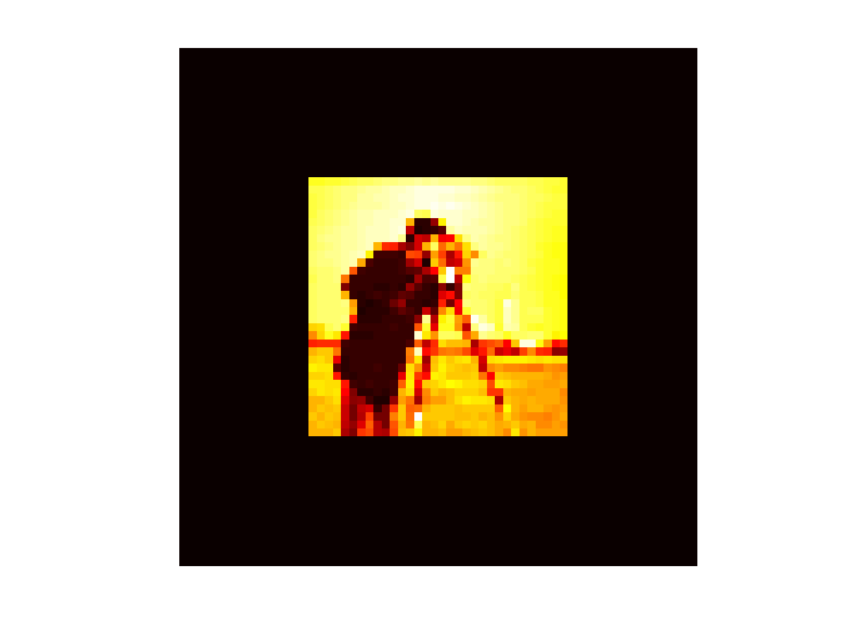
Figure 1: Object $\psi$ ($64\times 64$) used to simulate diffraction data

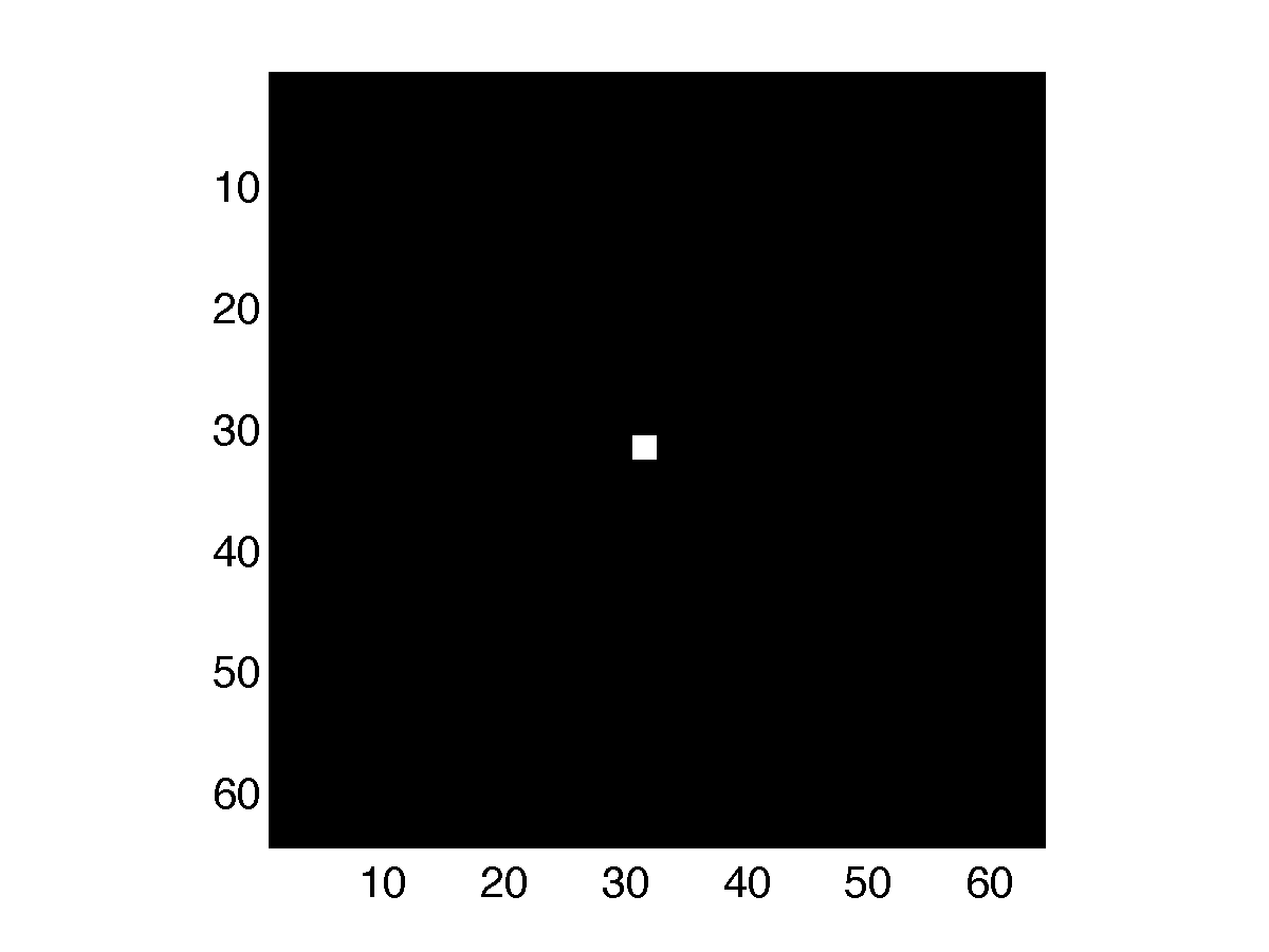
Figure 2: Each column of the matrix $T$ extracts an area of $2\times 2$ pixels out of an image of ($64\times 64$) pixels.

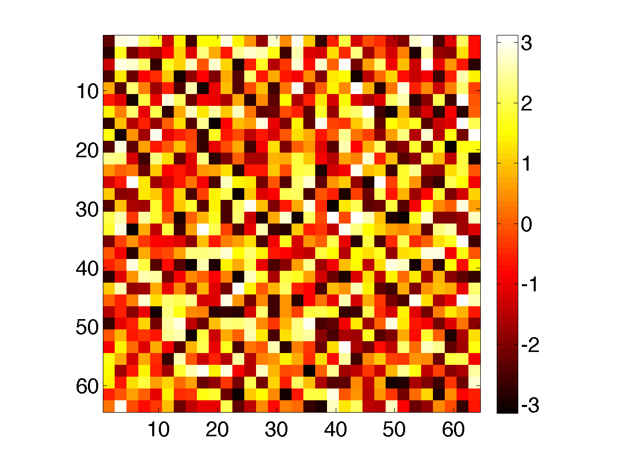
Figure 3: Random perturbation: ($64\times 64$) phases generated by $32\times 32$ random phases each spread over a bin of ($2\times 2$) pixels.

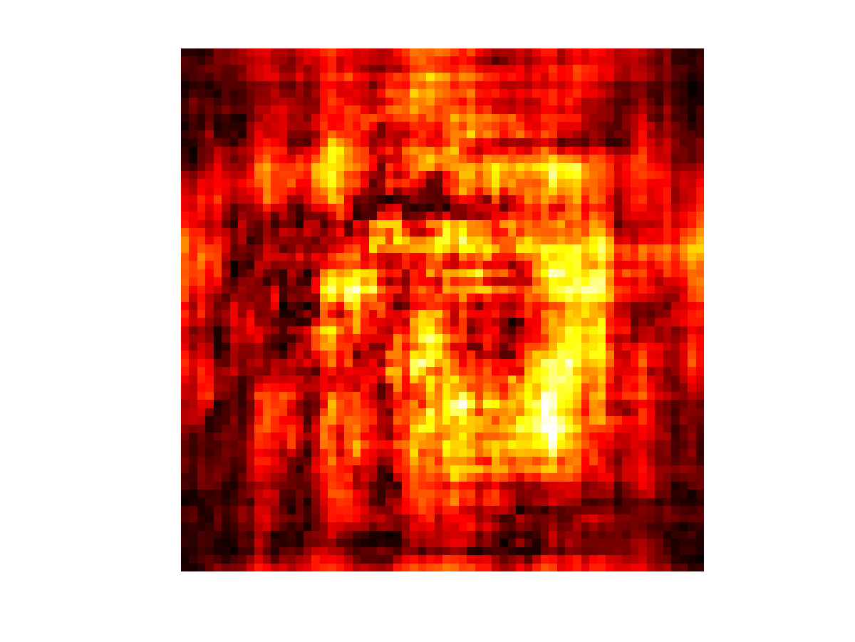
Figure 4: Image in real space ($\left|\bm{F}^{\ast}{\bf z}\right|$) after random phase perturbation (Fig. 6)

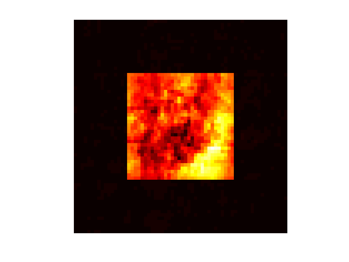
Figure 5: Image in real space after random phase perturbation (Fig. 6), using Eq. 6 updates ( $\left|\bm{F}^{\ast}(P_{\bm{a}}P_{S})^{1000}{\bf z}\right|$).

Figure 6: Image in real space after one step of Eqs. (15,16) update.

References

- Marchesini et al. (2012) S. Marchesini, A. Schirotzek, F. Maia, and C. Yang, (2012), arXiv:1209.4924 [physics.optics] .
- Marchesini (2007) S. Marchesini, Rev Sci Instrum 78, 011301 (2007), arXiv:physics/0603201 .
- Singer (2011) A. Singer, Applied and Computational Harmonic Analysis 30, 20 (2011), arXiv:0905.3174 .
- Waldspurger et al. (2012) I. Waldspurger, A. d’Aspremont, and S. Mallat, ArXiv (2012), arXiv:1206.0102 [math.OC] .
- Alexeev et al. (2012) B. Alexeev, A. S. Bandeira, M. Fickus, and D. G. Mixon, (2012), arXiv:1210.7752 [cs.IT] .