Modulational instabilities in lattices with power-law hoppings and interactions

Abstract

We study the occurrence of modulational instabilities in lattices with non-local, power-law hoppings and interactions. Choosing as a case study the discrete nonlinear Schrödinger equation, we consider one-dimensional chains with power-law decaying interactions (with exponent $\alpha$) and hoppings (with exponent $\beta$): An extensive energy is obtained for $\alpha,\beta>1$. We show that the effect of power-law interactions is that of shifting the onset of the modulational instabilities region for $\alpha>1$. At a critical value of the interaction strength, the modulational stable region shrinks to zero. Similar results are found for effectively short-range nonlocal hoppings ($\beta>2$): At variance, for longer-ranged hoppings ($1<\beta<2$) there is no longer any modulational stability. The hopping instability arises for $q=0$ perturbations, thus the system is most sensitive to the perturbations of the order of the system’s size. We also discuss the stability regions in the presence of the interplay between competing interactions - (e.g., attractive local and repulsive nonlocal interactions). We find that noncompeting nonlocal interactions give rise to a modulational instability emerging for a perturbing wave vector $q=\pi$ while competing nonlocal interactions may induce a modulational instability for a perturbing wave vector $0<q<\pi$. Since for $\alpha>1$ and $\beta>2$ the effects are similar to the effect produced on the stability phase diagram by finite range interactions and/or hoppings, we conclude that the modulational instability is “genuinely” long-ranged for $1<\beta<2$ nonlocal hoppings.

I Introduction

The investigation of the effects of the interplay between discreteness and nonlinearity is a long-standing argument of research in the study of the dynamical properties of nonlinear lattice models flach98 ; braun98 ; hennig99 ; ablowitz04 ; campbell04 ; malomed06 ; flach08 . A typical feature exhibited by nonlinear classical Hamiltonian lattices is the existence of discrete breathers, i.e. time-periodic and space-localized solutions of the equations of motion. The study of their dynamical stability, as well as their robustness in long transient processes and thermal equilibrium, has been the subject of an intense experimental and theoretical work flach08 .

The interplay between discreteness and nonlinearity is also crucial for the occurrence of modulational instabilities (MI), well known in the theory of nonlinear media flach98 ; braun98 . MI are dynamical instabilities characterized by an exponential growth of arbitrarily small fluctuations resulting from the combined effect of dispersion and nonlinearity. The occurrence of modulational instabilities has been studied in a number of physical systems, ranging from fluid dynamics benjamin67 to nonlinear optics agrawal07 . The role and the consequences of the MI in the dynamics of discrete systems have been extensively studied: The MI was discussed in the context of the discrete nonlinear Schrödinger equation (DNLSE) kivshar92 , which is a paradigmatic lattice model kevrekidis01 used to study nonlinear discrete dynamics hennig99 ; ablowitz04 . The DNLSE is commonly used to describe the effective dynamics in different physical systems of interest, including the dynamics of ultracold atoms in optical lattices trombettoni01 and optical waveguide arrays eisenberg98 . For ultracold bosons in optical lattices the onset of MI was analytically predicted smerzi02 and experimentally observed cataliotti03 , and in nonlinear waveguide arrays the experimental observation of the MI was also reported meier04 .

In this paper we study the occurrence of MI in the DNLSE in the presence of non-local long-range hoppings and interactions. A motivation for such a study comes from experiments with ultracold dipolar bosonic gases lahaye09 ; trefzger11 which have been Bose condensed recently by several groups griesmaier05 ; bismut10 ; lu11 , from the attainment of quantum degeneration for ensembles of polar molecules ospelkaus10 , and from the recent experimental investigations of strongly interacting Rydberg gases heidemann08 ; schauss12 ; saffman10 . Since the interaction potential in (di)polar gases decay as a power law $1/r^{3}$ (for Rydberg gases interacting through van der Waals interactions as $1/r^{6}$), recent experiments with dipolar gases in optical lattices muller11 ; billy12 ; depaz12 , as well as the realization of long-lived dipolar molecules in a three-dimensional periodic potential chotia11 and in perspective the dynamics of Rydberg atoms in optical lattices henkel10 ; viteau12 , open the possibility to study DNLSE with non-local interactions.

Our other motivation is related to the wide interest in systems with long-range interactions leshouches10 . In these systems the range of interaction of the constitutive units is not bounded. A typical form of interactions, relevant for a number of systems ranging from gravitational ones to dipolar magnets and gases, is provided by the power-law decay $1/r^{\gamma}$ (e.g. for gravitational systems $\gamma=1$) where $r$ is the distance among the constituents. For statistical mechanics models, like the Ising or more generally the $O(n)$ models, the possibility to have power-law couplings makes possible the appearance of a rich phase diagram fisher72 ; sak73 ; luijten02 .

A first criterion to determine the long-rangedness of a system with power-law decaying interaction is the comparison with the dimension $d$ of the space; as $\gamma$ is smaller than or equal to $d$, if the system is homogeneous and the interaction favours homogeneity we obtain a diverging energy density, thus to obtain a well defined thermodynamic limit (if relevant) a rescaling of the energy is in order (the so called Kac rescaling) ruffo09 . In the following we will refer to this region as the non-extensive long-range region. If $\gamma$ is larger than $d$ the energy of the system is extensive and it is normal to individuate a value of $\gamma$, which we denote by $\gamma^{\ast}$, such that for $\gamma>\gamma^{\ast}$ the system behaves as a short-range system. Since it is $\gamma^{\ast}>d$, there is a region of values of $\gamma$, given by $d<\gamma<\gamma^{\ast}$, in which the behavior of the system significantly differs from the properties of the same system with short-range interactions, although the energy is extensive. Such a region is the extensive long-range region, also referred to as the weak-long-range region ruffo09 , where “weak” refers to the extensivity of the energy. The actual value of $\gamma^{\ast}$ depends on the specific model and the dimension: For $O(n)$ models in $d=1$ it is $\gamma^{\ast}=2$ kosterlitz76 ; spohn99 .

Both the thermodynamics and the dynamics of long-range interacting systems are extremely interesting leshouches10 ; ruffo09 . In particular, in the long-range region the dynamical evolution evidences that the system may stay in a quasi-stationary metastable state (different from the thermal equilibrium one) for a time exponentially growing with the size of the system. Such a metastable state is reached after a short-time dynamics, referred to as violent relaxation ruffo09 .

While the main bodies of the studies on the dynamics of nonlinear lattices have dealt with short-ranged systems, the extensions of these results to long-ranged systems appeared in the literature addressing the properties of discrete systems with different kinds of non-local dispersion or non-local nonlinear interaction we mentioned gaididei97 ; flach98_2 ; christiansen98 ; mingaleev00 ; fratalocchi05 and focused on the existence and stability of localized excitations (for a recent review on nonlinear waves in lattices see kevrekidis11 ).

The purpose of the present paper is to study how modulational instabilities emerge in nonlinear lattices with non-local interactions and hoppings, aiming both at unveiling if (and in which conditions) short time dynamical instabilities occur in nonlinear lattices and at clarifying the nature of the emerging modulational instability. We choose the DNLSE as a case study not only due to its paradigmatic usefulness, but also due to its relation with $XY$ [i.e., $O(2)$] models: When the fluctuation of the number of particles are frozen, the kinetic term in the DNLSE energy is basically the $XY$ model (see the discussion in Sec. II). This is the reason why we choose to consider not only power-law interactions (as it is relevant for experiments with ultracold dipolar bosons in optical lattices), but also power-law hoppings [which corresponds to power-law couplings in $O(2)$ models]. Using the DNLSE we study the modulationally stable and unstable regions in the presence of power-law non-local interactions and hoppings, discussing also the interplay between local and non-local interactions, e.g. local attraction and non-local repulsion.

The plan of the paper is as follows. In Sec. II, we introduce the DNLSE with long-range hoppings and interactions and discuss its relation with other statistical mechanics models. In Sec. III we derive the Bogoliubov spectrum of elementary excitations, present the general framework for the determination of the stability regions in presence of power-law interactions and hoppings and specialize it to the analysis to the short-range limit reminding the known results of the MI analysis kivshar92 ; smerzi02 . Our findings for power-law interactions are presented in Sec. IV where we also consider the case of attractive and competing local and non-local interactions. Sec. V deals with a system with non-local hopping and local interaction which presents some peculiar features with respect to the long-range interaction which are further investigated in VI. The physical applications of our results, in particular to ultracold dipolar gases in optical lattices, are discussed in Sec. VII, while our conclusions are in Sec. VIII.

II The DNLSE with long-range interactions and hoppings

The DNLSE with non-local interactions and hoppings reads

$$i\hbar\frac{\partial\psi_{j}}{\partial\tau}=-\sum_{m}t_{j,m}\psi_{m}+\sum_{m}V_{j,m}\mid\psi_{m}\mid^{2}\psi_{j}.$$ (1)

In Eq. (1) $\tau$ is the time and the indices $j,m$ denote the sites of a lattice. For simplicity we assume that the lattice is one dimensional, but the subsequent analysis can be extended to higher dimensional lattices. The indices $j,m$ then assume the values $j,m=0,\ldots,L-1$ ($L$ is the number of the sites, taken to be even). Periodic boundary conditions will be also assumed, so that the wavefunction satisfies the condition $\psi_{j}=\psi_{j+L}$. The Hamiltonian corresponding to Eq. (1) reads

$$H_{\text{DNLSE}}=-\sum_{j,m}\psi_{j}^{\ast}t_{j,m}\psi_{m}+\frac{1}{2}\sum_{j,m}\mid\psi_{j}\mid^{2}V_{j,m}\mid\psi_{m}\mid^{2}.$$ (2)

We denote the diagonal interaction by

$$V_{j,j}=U,$$ (3)

and the next-neighbor interaction as

$$V_{j,j+1}=V.$$ (4)

The interaction coefficients $V_{j,m}$ in Eq. (1) are assumed to be power-law decaying with exponent $\alpha$, i.e. $\sim 1/\mid m-j\mid^{\alpha}$. Since $V_{m,j}=V_{j,m}$, implementing the periodic boundary conditions amounts to require that $V_{j,m}=V_{\left(j+n\right)\mod L,\left(m+n\right)\mod L}$, where $j\leq m$ and $n=1,\ldots,L-1$. We have therefore

$$V_{0,m}=\left\{\begin{array}[]{ll}U&m=0,\\ \frac{V}{m^{\alpha}}&m=1,\ldots,\frac{L}{2}\\ \frac{V}{\left(L-m\right)^{\alpha}}&m=\frac{L}{2}+1,\ldots,L-1\end{array}\right.$$ (5)

The non-local hopping rates $t_{j,m}$ will be also assumed to be power-law decaying with exponent $\beta$. We consider vanishing diagonal hopping ($t_{j,j}=0$) and a nearest-neighbor hopping

$$t_{j,j+1}=t.$$ (6)

Therefore, with periodic boundary conditions we have

$$t_{0,m}=\left\{\begin{array}[]{ll}0&m=0,\\ \frac{t}{m^{\beta}}&m=1,\ldots,\frac{L}{2}\\ \frac{t}{\left(L-m\right)^{\beta}}&m=\frac{L}{2}+1,\ldots,L-1\end{array}\right.$$ (7)

Since we want a finite expression for the energy per particle, we will consider

$$\alpha>1\,,\qquad\,\beta>1.$$ (8)

To treat the cases $\alpha\leq 1$ or $\beta\leq 1$ one should do a Kac rescaling, as it is usually done in statistical mechanics models with nonextensive long-range interactions ruffo09 : e.g., for $\beta\leq 1$ one has to perform the substitution

$$t_{j,m}\to\frac{t_{j,m}}{\sum_{m}\frac{1}{m^{\beta}}}.$$ (9)

A non-extensive ground-state energy is found in our case by $\alpha\to 1$ and/or $\beta\to 1$: The region $1<\beta<2$ is the weak-long-range hopping region. Recall that such region is of high interest in the study of statistical mechanics models with long-range couplings. Let us consider an Ising model of the form

$$H_{\text{Ising}}=-\sum_{i,j}J_{ij}s_{i}s_{j},\,\,\,\,\,\,\left(s_{i}=\pm 1\right),$$ (10)

with power-law couplings $J_{ij}\propto 1/\mid i-j\mid^{\gamma}$. As usual, $i,j$ denote the sites of a lattice with dimension $d$. It is well known that for nearest-neighbor couplings (formally corresponding to $\gamma=\infty$) there is order at finite temperature only if $d\geq 2$ yeomans92 . However, if the interactions are sufficiently long-ranged it is possible to have a phase transition at finite temperature between a ferromagnetic and a paramagnetic phase dyson69 ; thouless69 even for $d=1$: If $\gamma>2$, then the critical temperature $T_{c}$ is vanishing (as in any short-range Ising chain yeomans92 ), while for $\gamma\leq 1$ the energy is non-extensive. After the Kac rescaling one easily sees that for $\gamma\leq 1$ there is a phase transition having the critical exponents of the mean-field universality class (see e.g. lebellac91 ). For $\gamma$ between $1$ and $2$ (weak-long-range region) there is a phase transition at a finite critical temperature. For $\gamma=2$ a Kosterlitz-Thouless transition takes place thouless69 ; anderson71 ; luijten01

Before moving on to the derivation of the Bogoliubov spectrum of elementary excitations, we pause here to discuss the relation between the DNLSE (1) and a model widely used in the treatment of long-range systems, i.e. the Hamiltonian mean field (HMF) model ruffo09 . We observe that the DNLSE Hamiltonian (2) can be written as the sum of a kinetic term $H_{\text{kin}}$ and an interaction term $H_{\text{int}}$. The kinetic part reads $H_{\text{kin}}=-\sum_{j,m}\psi_{j}^{\ast}t_{j,m}\psi_{m}$: By writing $\psi_{j}$ in terms of the local density $n_{j}$ and phase $\theta_{j}$, i.e., $\psi_{j}=\sqrt{n_{j}}e^{i\theta_{j}}$ the kinetic part reads then $H_{kin}=-\sum_{j,m}t_{j,m}\sqrt{n_{j}n_{m}}\cos{\left(\theta_{j}-\theta_{m}\right)}$. One sees than when the number fluctuations are frozen, i.e. $n_{j}\approx\rho$ (where $\rho$ is the average number of particles per site), the DNLSE Hamiltonian reduces to the potential energy (and it has the same equilibrium properties) of the HMF model ruffo09

$$H_{\text{HMF}}=-\sum_{j,m}J_{j,m}\cos{\left(\theta_{j}-\theta_{m}\right)},$$

(where $J_{j,m}\equiv t_{j,m}\rho$), which is nothing but a long-range $XY$ model. This result is of course expected in the sense that interacting bosons on a lattice are in the $XY$ universality class, and interacting bosons with long-range hoppings have to be in the universality class of the long-range $XY$ model.

III Modulational stability analysis in presence of long-range interactions and hoppings

We study in this section the Bogoliubov spectrum of elementary excitations, describing the energy of small perturbations with (quasi)momentum $q$ on top of a plane-wave state with (quasi)momentum $k$ kivshar92 . The final part of the section is devoted to briefly recall the results of the short-range limit ($V=0$ and $\beta\to\infty$, i.e., only nearest-neighbor hopping).

The stationary solutions of Eq. (1) are plane-waves

$$\psi_{j}(\tau)=\psi_{0}\exp{[i(kj-\nu\tau)]}:$$

$\nu$ is the chemical potential given (for $L\to\infty$) by

$$\hbar\nu=-2t\ell_{\beta}(k)+\rho\left[U+2V\zeta\left(\alpha\right)\right].$$ (11)

In Eq. (11) $\rho$ is the plane-wave density ($\rho\equiv\mid\psi_{0}\mid^{2}$); furthermore $\zeta\left(\alpha\right)$ is the Riemann zeta function

$$\zeta\left(\alpha\right)=\sum_{m=1}^{\infty}\frac{1}{m^{\alpha}}$$ (12)

and we introduce the function

$$\ell_{\beta}(k)=\sum_{m=1}^{\infty}\frac{\cos{(mk)}}{m^{\beta}}.$$ (13)

Some useful properties of the function (13) are recalled and discussed in the Appendix A.

The stability analysis of plane-waves’ stationary solutions can be carried out by perturbing the carrier waves as

$$\psi_{j}(\tau)=\left[\psi_{0}+u(\tau)e^{iqj}+v^{\ast}(\tau)e^{-iqj}\right]e^{i(kj-\nu t)}.$$

Retaining only the terms proportional to $u/\psi_{0}$ and $v/\psi_{0}$, one gets

$$i\hbar\frac{d}{d\tau}\left(\begin{array}[]{c}u\\ v\end{array}\right)=\left(\begin{array}[]{cc}{\cal A}&{\cal C}\\ -{\cal C}^{\ast}&-{\cal B}\end{array}\right)\,\left(\begin{array}[]{c}u\\ v\end{array}\right).$$ (14)

The quantities ${\cal A}$, ${\cal B}$, and ${\cal C}$ in Eq. (14) are defined by

$${\cal A}=2t\left[\ell_{\beta}\left(k\right)-\ell_{\beta}\left(k+q\right)\right]+\rho\tilde{V}_{q},$$ (15)

$${\cal B}=2t\left[\ell_{\beta}\left(k\right)-\ell_{\beta}\left(k-q\right)\right]+\rho\tilde{V}_{q}$$ (16)

and

$${\cal C}=\psi_{0}^{2}\tilde{V}_{q}.$$ (17)

In the previous expressions, $\tilde{V}_{q}$ is the Fourier transform of the interaction (5): For finite $L$ it is

$$\tilde{V}_{q}=\sum_{m=0}^{L-1}V_{0,m}\,e^{iqm}.$$

For $L\to\infty$ one obtains

$$\tilde{V}_{q}=U+2V\ell_{\alpha}\left(q\right).$$ (18)

From Eq. (14) it follows that the excitation spectrum (i.e., the Bogoliubov dispersion relation) for the DNLSE with power-law hoppings and interactions is

$$\hbar\omega_{\pm}=\frac{{\cal A}-{\cal B}}{2}\pm 2t\sqrt{{\cal I}},$$ (19)

where $\omega_{\pm}=\omega_{\pm}(k;q)$ is a function of $k$ and $q$ (respectively momentum of the perturbed and perturbing plane-waves). Furthermore

$${\cal I} =\frac{1}{4}\,\left\{2\ell_{\beta}(k)-\ell_{\beta}(k+q)-\ell_{\beta}(k-q)\right\}^{2}+$$

$$+\frac{\rho\tilde{V}_{q}}{2t}\,\left\{2\ell_{\beta}(k)-\ell_{\beta}(k+q)-\ell_{\beta}(k-q)\right\}=$$

$$=\mathcal{F}(k;q)\left(\mathcal{F}(k;q)+\frac{\rho\tilde{V}_{q}}{t}\right),$$ (20)

where we introduced the function $\mathcal{F}(k;q)=\left\{2\ell_{\beta}(k)-\ell_{\beta}(k+q)-\ell_{\beta}(k-q)\right\}/2$. In the following we will use the convenient dimensionless parameters

$$\bar{U}=\frac{U\rho}{t}\,,\qquad\,\bar{V}=\frac{V\rho}{t}.$$ (21)

In terms of the parameters $\bar{U}$, $\bar{V}$, the quantity $\rho\tilde{V}_{q}/t$ entering Eq. (20) reads

$$\frac{\rho\tilde{V}_{q}}{t}=\bar{U}+2\bar{V}\ell_{\alpha}(q).$$ (22)

The carrier wave becomes modulationally unstable when the eigenfrequencies $\omega_{\pm}$ in Eq. (19) acquire a finite imaginary part: The condition for stability is then ${\cal I}\geq 0$. A momentum $k$ is then modulationally stable if for each $q$ the eigenfrequencies $\omega_{\pm}$ are real, otherwise if it exists a $q$ such that ${\cal I}<0$ then $k$ will be modulationally unstable. Since the eigenvalues are unaffected by substituting $k$ with $-k$ and $q$ with $-q$, we will consider $k$ and $q$ both belonging to the interval $[0,\pi]$. Notice that for $q=0$ it is ${\cal I}=\omega_{\pm}=0$.

When a momentum $k$ is modulationally unstable, there will be some momentum $q$ for which $\omega_{+}(k;q)$ and $\omega_{-}(k;q)$ have an imaginary part $\mathrm{Im}\,\omega_{\pm}(k;q)$. For those values of $k$ and $q$ we write

$$\Gamma(k;q)=\mid\mathrm{Im}\,\omega_{\pm}(k;q)\mid$$ (23)

to quantify how unstable is the perturbed plane-wave [notice that the imaginary parts of $\omega_{+}(k;q)$ and $\omega_{-}(k;q)$ are by definition opposite in sign and equal in modulus]. For $k$ unstable we will use the notation $\Gamma_{\text{max}}(k)=\max_{q}{\Gamma(k;q)}$, where the $\max$ is taken on all the $q$ such that $\omega^{2}(k;q)<0$. The value of $q$ for which the maximum value of $\Gamma(k;q)$ is obtained will be denoted by $q_{\text{max}}$ [i.e., $\Gamma_{\text{max}}(k)=\Gamma(k;q_{\text{max}})$].

III.1 The short-range limit

In this section we review the results and the region of stability for the short-range limit, having only local interaction ($\bar{V}=0$) and nearest-neighbor hopping: $t_{j,j\pm 1}=t$ and $t_{j,m}=0$ for $m\neq j\pm 1$ [formally this is the limit $\beta\to\infty$ in Eq. (7)].

It has been shown in kivshar92 that the onset of MI occurs at $k_{\text{cr}}=\pi/2$, i.e., the momenta $k<\pi/2$ are modulationally stable, while for $k>\pi/2$ are unstable. The quantity ${\cal I}$, defined in Eq. (20) and giving the stability regions reads

$${\cal I}=4\cos^{2}{k}\sin^{4}{\frac{q}{2}}+2\bar{U}\cos{k}\sin^{2}{\frac{q}{2}}.$$ (24)

One readily sees that the momenta $k<\pi/2$ are stable. For $k>\pi/2$ all the momenta $k$ are unstable, irrespective of $U$. However, one sees that for $k>\pi/2$ and $\bar{U}>2$ each $q$ is unstable, while for $\bar{U}<2$ there are stability regions: These stable regions are found to be bounded by the regions in which $q$ is between $q_{\text{cr}}$ and $\pi$ and $k$ is between $k_{\text{cr}}$ and $\pi$, where

$$k_{\text{cr}}=\pi-\arccos{\frac{\bar{U}}{2}}$$

and

$$q_{\text{cr}}=2\arcsin{\sqrt{\frac{\bar{U}}{2}}}.$$

The resulting plots of stable and unstable regions for $\bar{U}>2$ and $\bar{U}<2$ are in Fig. 1, where we plot as well as contour plot the value of $\Gamma(k;q)$ in the unstable regions (the larger $\Gamma$, the more unstable is the dynamics). In Fig. 2 we also plot as a solid line the values $q_{\text{max}}(k)$ for which the maximum value of $\Gamma$, at the fixed $k$, is reached.

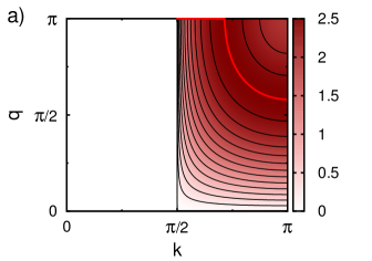
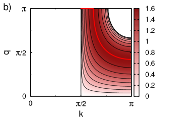
Figure 1: (Color online) Stable (white) and unstable [gray, (red)] regions for the short-range DNLSE ($\bar{V}=0$ and only nearest-neighbor hoppings) for $\bar{U}=2.5$ (a) and $\bar{U}=1.5$ (b) in the $k$ (carrier wave momentum) $q$ (perturbing wave momentum) plane. The absolute value of the imaginary part of the frequencies $\Gamma(k;q)$ is depicted [from light to dark as $\Gamma(k;q)$ increases]. The continuous lines are equispaced isolines whose spacing is set to $0.2$. The thick (red) line indicates the position of $q_{\text{max}}$.

IV Power-law interactions

In this section we consider the case of power-law interactions in the presence of (local) nearest-neighbor hoppings ($t_{j,j\pm 1}=t$ and $t_{j,m}=0$ for $m\neq j\pm 1$). One has then

$${\cal I}=4\cos^{2}{k}\sin^{4}{\frac{q}{2}}+2\cos{k}\sin^{2}{\frac{q}{2}}\left[\bar{U}+2\bar{V}\ell_{\alpha}(q)\right].$$ (25)

We consider only the cases where $\bar{V}>0$ and the local interaction $\bar{U}$ can be either or positive or negative. The cases where $\bar{V}$ is negative can be easily derived from the cases where $\bar{V}>0$ by noticing that under the following transformation

$$\begin{array}[]{ccc}\cos(k)&&-\cos(k)\\ \bar{U}&\rightarrow&-\bar{U}\\ \bar{V}&&-\bar{V}\\ \end{array}$$ (26)

one obtains the same dependence on $q$ and $\alpha$ of the stability conditions that one has when $V$ is positive. For example, if for a fixed value $\bar{V}=V_{0}>0$ and $\bar{U}=U_{0}<0$ one has that the momentum $\tilde{k}$ is stable, then momentum $\pi-\tilde{k}$ will also be stable for $\bar{V}=-V_{0}<0$ and $\bar{U}=-U_{0}>0$.

IV.1 Repulsive interactions: $U>0$, $V>0$

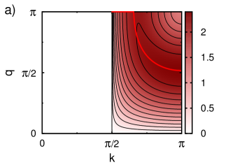
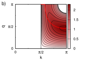
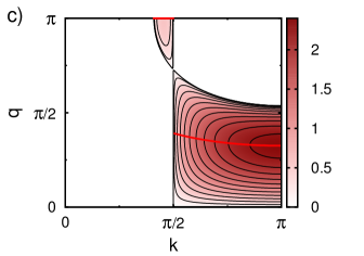
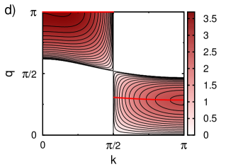
Figure 2: (Color online) Stability in the $k$-$q$ plane (see caption of Fig. 1) for power-law interactions in presence of local nearest-neighbor hoppings with $\alpha=1.5$ and $\bar{U}=2.5$. We plot $\Gamma(k;q)$ for the four values of $\bar{V}=0.2$, $0.5$, $2$, and $4$ in panels $a$, $b$, $c$, and $d$, respectively.

We consider here $U$ and $V$ to be positive. Since $\partial\ell_{\alpha}/\partial q\leq 0$ for $\alpha>1$ and $q\in[0,\pi]$, one can show the following:

• For

  $$\bar{U}>2\bar{V}\zeta(\alpha)(1-2^{1-\alpha})$$

  the momenta $k<\pi/2$ are stable.

• For

  $$\bar{U}<2\bar{V}\zeta(\alpha)(1-2^{1-\alpha})-2$$

  the momenta $k<\pi/2$ are unstable.

It follows that the critical value $k_{\text{cr}}$ as a function of $\bar{V}$ is given by

$$\cos{k_{\text{cr}}}=\bar{V}\zeta(\alpha)(1-2^{1-\alpha})-\frac{\bar{U}}{2},$$ (27)

i.e., for $2\bar{V}\zeta(\alpha)(1-2^{1-\alpha})-2>\bar{U}$ one has $k_{\text{cr}}=0$. For $k>\pi/2$ it is easy to see that all momenta are unstable against perturbations at $q=0$. Notice that for $\alpha\to\infty$ (i.e., for the model having only on-site and nearest-neighbor interactions) Eq. (27) reads $\cos{k_{\text{cr}}}=\bar{V}-\bar{U}/2$.

The instability regions are depicted in Fig. 2 as $V$ is increased - for $\bar{U}>2$, one can identify four regions. For $2\bar{V}\mid\ell_{\alpha}(\pi)\mid+2<\bar{U}$ with $\ell_{\alpha}(\pi)=\zeta(\alpha)(1-2^{1-\alpha})$, then the momenta $k$ larger than $\pi/2$ (smaller than $\pi/2$) are unstable for all $q$. Increasing $\bar{V}$, one has that for $\bar{U}-2<2\bar{V}\mid\ell_{\alpha}(\pi)\mid<\bar{U}$ a stable region forms around $k=\pi,q=\pi$, while for $\bar{U}<2\bar{V}\mid\ell_{\alpha}(\pi)\mid<\bar{U}+2$ an unstable region appears close to $q=\pi$ for momenta $k$ between $k_{\text{cr}}$ given by Eq. (27) and $\pi/2$. When $\bar{U}+2>2\bar{V}\mid\ell_{\alpha}(\pi)\mid$, then all the $k$ becomes unstable and the instability starts from $q=\pi$. Therefore, the plane wave $k_{\text{cr}}$ is rendered unstable by the wave vector $q=\pi$, thus the system is the most sensitive to short wavelength perturbations.

The behavior of $k_{\text{cr}}$ is plotted in Fig. 3. The analytical prediction (27) (valid for $\alpha>1$) is compared for $\alpha=3$ against numerical findings obtained numerically solving the DNLSE finding a very good agreement [for comparison we also plot the analytical result (27) for $\alpha\to\infty$]. The numerical solution has been obtained on a finite-size system (we choose $L=512$) whose coherence has been monitored by inspecting the absolute value of the following order parameter smerzi02

$$\varphi(\tau)=\frac{1}{L}\sum_{k}|\tilde{\psi}_{k}(\tau)|^{2}e^{ik},$$ (28)

where $\tilde{\psi}_{k}(\tau)=-\frac{1}{\sqrt{L}}\sum_{m}\psi_{m}(\tau)e^{-ikm}$ is the Fourier transform of the wave functions. The initial wavefunction $\psi_{j}(\tau=0)$ is chosen as a plane wave with wave vector $k$ perturbed by the highest frequency wavevector $\psi_{j}(\tau=0)=e^{ikj}+\epsilon e^{iqj}$, with $q=\pi$ (notice that $q_{max}=\pi$ for non-competing interactions, as one can see from Fig. 2). The ratio between the amplitudes of perturbing and perturbed wave functions is set to be $\epsilon=10^{-3}$ with $\rho=1$. As we can see in the left panel of Fig. 4, if prepared in a modulationally unstable initial state, the system loses coherence after a time which diverges as we approach the momentum $k_{\text{cr}}$: Denoting with $\tau_{I}$ the time after which the instability is observed using the order parameter (28), and noticing that the quantity (20) is vanishing (at $q=\pi$) as $\sim(k-k_{\text{cr}})$, one can estimate $k_{\text{cr}}$ from the numerical data using the dependence $\tau_{I}\propto\left(k-k_{\text{cr}}\right)^{-1/2}$ (see Fig. 4, right panel). This divergence has been used to extract the numerical values of $k_{\text{cr}}$ shown in Fig. 3.

Figure 3: The solid line represents $k_{\text{cr}}$ vs $\bar{V}$ from Eq. (27) (in the figure $\bar{U}=1$ and $\alpha=3$). The dots represent values obtained by direct simulation of the DNLSE, see the text for details (errors are smaller than the symbols). Notice that for $\bar{U}=1$ and $\alpha\to\infty$ one has $k_{\text{cr}}=\pi/2$ for $\bar{V}<0.5$ and $k_{\text{cr}}=0$ for $\bar{V}>1.5$. The dotted line is the analytical value of $k_{\text{cr}}$ vs $\bar{V}$ from Eq. (27) with $\alpha\to\infty$ and $\bar{U}=1$.

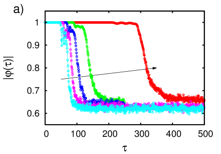
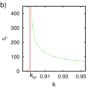
Figure 4: Time evolution (on the left) of the modulus of the order parameter $\varphi$, defined in Eq.  (28), for five different values (from left to right $k=77$, $76$, $75$, $74$, $73$, $72$ in units of $2\pi/L$ with $L=512$) of carrier plane-wave wavevector for the DNLSE with parameters $\bar{U}=1$, $\bar{V}=1.25$, and $\alpha=3$. The lifetimes of the initial states are depicted in the right part of the figure. These times have been fitted with a function $\tau=\text{const}(k-k_{\text{cr}})^{-1/2}$ (dotted line) to obtain the a numerical estimates of $k_{\text{cr}}$ (vertical line).

IV.2 Competing interactions: $U<0$, $V>0$

For $k<\frac{\pi}{2}$ a necessary condition for stability is given by $|\bar{U}|<2\bar{V}\zeta(\alpha)$ that is obtained by analyzing the stability at $q=0$. The critical momentum is given by

$$k_{\text{cr}}=\min_{q\in[0,\pi]}\left[\arccos\left(\frac{\bar{U}+2\bar{V}\ell_{\alpha}(q)}{2\sin^{2}(\frac{q}{2})}\right)\right].$$ (29)

all momenta $k<k_{\text{cr}}$ are stable.

An important feature of the case with competing interactions is that the most unstable perturbations can arise for a value of $q^{\ast}$ different from $0$ and $\pi$ (i.e., $0<q^{\ast}<\pi$). In the following we determine for what conditions at the critical value $k_{\text{cr}}$ there is an instability at a $q_{max}=q^{\ast}\neq 0,\pi$. We will refer to these values of $q^{\ast}$ as to finite values for the occurrence of modulational instability: This is because the instability develops on a length scale $\sim 1/q^{\ast}$. It is intended that if the instability arises at $q=\pi$, this develops on a length scale of the order the lattice unit, while an instability at $q=0$ involves length of the order of the lattice size: The later of these will be the case for non-local hoppings with weak-long-range exponents $1<\beta<2$.

An example of a finite $q^{\ast}$ is shown in Fig. 5. To see how this can arise we analyze for simplicity the situation at $k=0$, which can be easily generalized to a finite value in the interval $0<k<\pi/2$. To observe an instability region like the one in Fig. 5 we have to impose that the equation

$$h(q)=|\bar{U}|$$ (30)

with

$$h(q)=2\sin\left(\frac{q}{2}\right)^{2}+2\bar{V}\ell_{\alpha}(q),$$ (31)

obtained from Eq. (25) by the substitution $k=0$, has exactly one finite solution for fixed values of the parameters $(\alpha,\bar{U},\bar{V})$ and no solutions for smaller values of $\bar{U}$. After some algebra one can derive a set of conditions on the coefficients $(\alpha,\bar{V})$ such that the curve $h(q)$ possesses one minimum. It turns out that, if $\bar{U}=\min_{q\in(0,\pi)}h(q)$, then there is a $q^{*}\in\left(0,\pi\right)$ such that the instability region is tangent to the $k=0$ axis. For smaller values of $\bar{U}$ the previous equation $h(q)=|\bar{U}|$ does not have any solution and one obtains a finite value of $k_{\text{cr}}$ given by Eq. (29).

We can thus assert that the presence of competing interactions may originate the wavelength $q^{*}$ smaller than $\pi$ (and larger than $\pi$), unlike the case of the noncompeting interaction examined in the previous section for which the system is most sensible to perturbations at $q=\pi$. This is a general feature of systems with competing interactions acting on different scales which, if properly tuned, give rise to the birth of a new intermediate lengthscale (in this case of the order of $1/q^{*}$). For similar phenomena ultimately leading to stripe formation and more generally spatially modulated patterns in different contexts see, e.g., seul95 ; chakrabarty11 .

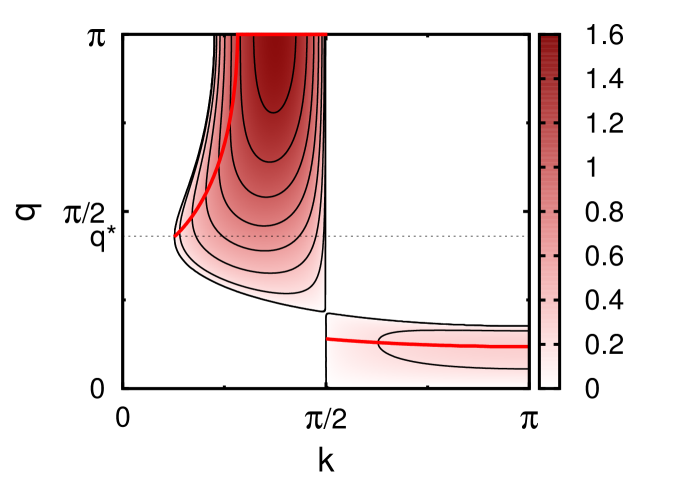
Figure 5: (Color online) Stability regions (see caption of Fig. 1) for the case of competing interactions with $\alpha=2$, $\bar{U}=-0.7$ and $\bar{V}=0.5$. The value of the most unstable $q$ which defines $k_{\text{cr}}$ is denoted by $q^{*}$.

For completeness we list the conditions on the parameters $(\alpha,\bar{V})$ such that the function $h(q)$ has a minimum for a finite value $q^{\ast}$ of the perturbing wavevector:

• for $1<\alpha\leq\alpha^{*}$

  $$\bar{V}<\frac{1}{(2-2^{1-\alpha})\zeta(\alpha)}$$ (32)

• for $\alpha^{*}<\alpha\leq 3$

  $$\bar{V}<\frac{1}{2(1-2^{3-\alpha})\zeta(\alpha-2)}$$ (33)

• for $\alpha>3$

  $$\frac{1}{2|\zeta(\alpha-2)|}<\bar{V}<\frac{1}{2(1-2^{3-\alpha})\zeta(\alpha-2)}.$$ (34)

(similar results are found for $0<k<\pi/2$). The value $\alpha^{*}$ in Eq. (33) is given by $\approx 1.513$, the unique solution of the equation:

$$2(1-2^{3-\alpha})\zeta(\alpha-2)=(1-2^{1-\alpha})\zeta(\alpha).$$ (35)

The condition ensuring the stability for every $k\in[\frac{\pi}{2},\pi]$ is given by:

$$|\bar{U}|>2\bar{V}\zeta(\alpha).$$ (36)

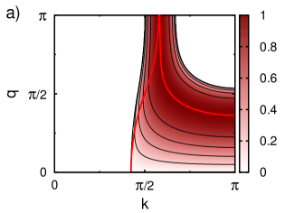
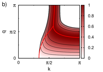
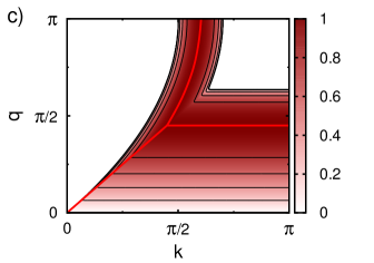
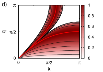
Figure 6: (Color online) Stability regions (see caption of Fig. 1) for the case of long-range hopping and local interaction $\bar{U}=1$ and $\bar{V}=0$. Panels (a), (b), (c), and (d) refer to the values of $\beta=4$, $3$, $2$, $1.5$.

V Power-law hoppings

In this section we consider the case of power-law nearest-neighbor hoppings, with exponent $\beta>1$. One has

$${\cal I} =\frac{1}{4}\,\left\{2\ell_{\beta}(k)-\ell_{\beta}(k+q)-\ell_{\beta}(k-q)\right\}^{2}+$$

$$+\frac{\bar{U}}{2}\left\{2\ell_{\beta}(k)-\ell_{\beta}(k+q)-\ell_{\beta}(k-q)\right\}=$$

$$=\mathcal{F}(k;q)(\mathcal{F}(k;q)+\bar{U})$$ (37)

While in the cases considered in Sec. IV the instabilities arise in the higher frequency range of $q$ [$q=\pi$] for non-competing interaction or at a finite value of $q$ [$q=q^{\ast}\in(0,\pi/2)$] for competing interactions, with non-local hoppings even the long-wavelength perturbations can affect significantly the stability properties of the system. This can be verified by an inspection of the behavior of ${\cal I}$ for small $q$. One finds for $q\to 0$

$${\cal I}\approx-\frac{\bar{U}q^{2}}{4}\frac{\partial^{2}\ell_{\beta}}{\partial k^{2}}.$$

The investigation of the behavior of the second derivative of $\ell_{\beta}(k)$ reveals that $\partial^{2}\ell_{\beta}/\partial k^{2}$ is positive for $1<\beta<2$ for each $k$. It follows that

$$k_{\text{cr}}=0\,\,\,\text{for}\,\,\,1<\beta<2,$$ (38)

i.e., the modulational stability regions shrink to zero in the weak-long-range regime, irrespective of $\bar{U}$ and $\bar{V}$ (we assume for simplicity in this section $\bar{U}>0$ and $\bar{V}>0$). The same analysis shows that for $\bar{V}=0$ the critical value $k_{\text{cr}}$ does not depend on the specific value of $\bar{U}$ for $\beta>2$. The above scenario is confirmed by Fig. 6 where we plot $\Gamma(k;q)$ as $\beta$ is increased. The values of $k_{\text{cr}}$ as a function of $\beta$ are plotted in Fig. 7. Notice that $k_{\text{cr}}$ tends to $\pi/2$ when the hopping exponent approaches the short range limit $\beta\to\infty$. As was done in Sec. IV we compare the analytical results with numerical simulations of the DNLSE obtaining a very good agreement.

Figure 7: Critical momentum $k_{\text{cr}}$ vs the power-law exponent $\beta$ of power-law hoppings with $\bar{V}=0$. Crosses are numerical data.

It should be stressed that the lifetimes of the modulationally unstable states in this case is typically longer than the ones encountered in Sec. IV. This will be supported in the next section where we directly compare instabilities arising from the long-range interaction and hopping, respectively.

When we introduce the long-range interaction $\bar{V}\neq 0$ the instability at $q=0$ due to long-range hopping remains unchanged since it is due to the vanishing of $\mathcal{F}(k;q)$ [see Eq. (37)], while the instabilities already discussed in Sec. IV are possibly generated. More precisely, an instability region at a finite value $q=q^{*}$ ($q^{*}=\pi$ for non-competing interactions) arises in the presence of $V$, however, for $V$ much smaller than $U$ (and smaller than a critical value $V_{c}$) then $k_{\text{cr}}$ is determined only by the $q=0$ instability driven by non-local hoppings and it is again given by the value at $V=0$, as shown in Fig. 7. When $V>V_{c}$ the contribution of both instabilities has to be taken into account to determine $k_{\text{cr}}$, with $q=0$ instabilities generated by long-range hopping and $q=\pi$ (or $q=q^{*}<\pi$ if the competition is sufficiently strong) instabilities due to the interaction. We comment on these scenarios in the next section.

VI Comparison of instabilities arising with non-local interactions and hoppings

The hopping instability described in Sec. V exhibits an important difference with the one arising from the interaction described in Sec. IV since $k_{\text{cr}}$ becomes unstable for $q=0$ perturbations, i.e., with a size of the order of the system’s size.

To compare the time scales on which these two kind of instabilities act we have considered a case where we switch on and off alternatively the long-range interaction and hopping (see Fig. 8). We prepare the two systems with a planewave $k$ slightly inside the instability region perturbed by a $q$ equaling $\pi$ and $2\pi/L$ (the widest available perturbation with a nonvanishing imaginary Bogoliubov frequency). By inspecting the contour plots [Figs. 8(a) and (b)] we foresee a longer lifetime for the instability induced by the non-local hoppings. This result is confirmed by numerical simulations, shown in panel $c$ of Fig. 8(c). This is a general feature of the long-range hopping instability: we observe that at the the critical value $k_{\text{cr}}$, by definition, $\Gamma(k_{\text{cr}};q_{\text{max}})=0$ both for non-local interaction and hoppings. However, entering the unstable region gives a vanishing value of $\Gamma(k;q)$ for $q=0$ and $k>k_{\text{cr}}$ and $\Gamma(k;q)\propto q$ for $q$ small for long-range hoppings. At variance for long-range interactions as $k$ is slightly larger than $k_{\text{cr}}$ then $\Gamma(k;q_{\text{inst}})$ generally acquires a finite value at the wavevector $q_{\text{inst}}$ at which the instability arises [with $q_{\text{inst}}=\pi$ for the non-competing case and $q_{\text{inst}}=q^{\ast}\in(0,\pi/2)$ for the competing one].

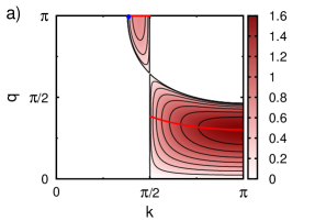
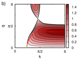
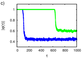
Figure 8: (Color online) Panels (a) and (b) are contour plots of $\Gamma(k;q)$ (see caption of Fig. 1) for $\bar{U}=\bar{V}=1$ and $\alpha=2.5$, $\beta=\infty$ (long-range interaction) and $\alpha=\infty$, $\beta=2.5$ (long-range hopping). In panel (c) we depict the time evolution of the order parameter defined in Eq. (28) for the initial conditions indicated in the contour plots with points. As we can see the long-range hopping instability, upper (green) curve, takes a much longer time to set in than the long-range interaction instability, lower (blue) curve.

Let us examine the peculiarities of the instabilities due to interaction and hopping and examine whether these may be reproduced with finite-range couplings or hoppings. As far as the long-range interaction is concerned, in the non competing case (examined in Sec. IV.1), we observe that the situation is not very different from the finite-range one with nearest-neighbor interaction ($\alpha\rightarrow\infty$). We can indeed find an effective nearest-neighbor $\tilde{\bar{V}}$ interaction giving rise to the same $k_{\text{cr}}$ [see Eq. (27)]:

$$\tilde{\bar{V}}=\bar{V}\zeta(\alpha)(1-2^{1-\alpha}).$$ (39)

Similarly in the case where the competition in present (described in Sec. IV.2) the case with $\alpha$ finite can be seen to be similar to the one obtained with $\alpha\rightarrow\infty$. In fact one can generate a new wavevector $q^{*}$ even when $\alpha\rightarrow\infty$, and thus the long-ranged-ness of the interaction is not actually playing a major role. As an example in Fig. 9(a) we have considered a case where a nearest-neighbor and next-to-nearest-neighbor interaction generates a stability diagram closely resembling the one shown in Fig. 5.

When we move to the hopping instabilities (examined in Sec. V) we observe that while a finite-range hopping can generate $q=0$ instabilities for $k<\pi$, the value of $k_{\text{cr}}$ is effectively limited by the range of the hopping and it is not $0$. This can be seen considering the hopping coefficients of range $R$, i.e., $t_{ij}=0$ for $\mid i-j\mid>R$. An example is given by $R=2$ where we set $t_{j,j\pm 1}\equiv t_{1}$, $t_{j,j\pm 2}\equiv t_{2}$. Explicit expressions (not reported here) for the stability regions can be derived repeating the analysis presented in Sec. III. It is possible to show that for a hopping of range $R$ then the critical momentum $k_{\text{cr}}$ can become as small as $\approx\pi/\left(2R\right)$ due to the $q=0$ instability. Thus for $\beta>2$ one can find a finite-range hopping with range $R$ to reproduce the critical value $k_{\text{cr}}$ and the stability regions of non-local hoppings with exponent $\beta$, while this is not the case for $1<\beta<2$. We conclude that the case $1<\beta<2$ where $k_{\text{cr}}=0$ is singled out as a case where the instability is genuinely due to the long-range nature of the hoppings. In Fig. 9(b) we depict the stability diagram of a case with the nearest- and next-to-nearest-neighbor hoppings mimicking the effect of long-range hopping shown in Fig. 6(a) and 6(b), with a finite value of $k_{\text{cr}}$.

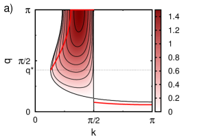
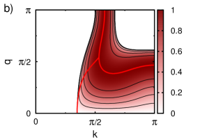
Figure 9: (Color online) Contour plots of $\Gamma(k;q)$ (see caption of Fig. 1) for models including only on-site interactions ($U$) and next- and next-to-nearest-neighbor interaction ($V$ and $V_{j,j+2}=V_{2}$) and hoppings ($t=1$ and $t_{j,j+2}=t_{2}$), respectively. Panel (a) refers to values $U=-0.8$, $V=0.4$, $V_{2}=0.05$, and $t_{2}=0$ while panel (b) refers to values $U=1$, $V=V_{2}=0$, and $t_{2}=0.2$.

VII Physical Applications

The cases we have analyzed can be applied to the study of modulational instability in a variety of physical systems characterized by non-local interaction and hopping coefficients. For example, the excitation transfer energy in molecular crystals and biopolymers exhibits a $1/r^{3}$ decay due to the dipole-dipole interaction davydov71 ; scott92 . The possibility of the inclusion of a non-local hopping is also present in DNA modeling (e.g., in the the Peyrard-Bishop model peyrard89 ), where the equation of motion for the transverse stretching of the hydrogen bonds connecting the bases facing each other contains a long-range hopping term due to the dipole-dipole interaction among hydrogen bonds resulting in a value $\beta=3$ cuevas02 . Another physical system characterized by non-local interactions is provided by ultracold atomic dipolar gases in optical lattices lahaye09 ; trefzger11 , for which experimental results recently appeared muller11 ; billy12 ; depaz12 . For dipolar bosons as ${}^{52}\mathrm{Cr}$ in the Bose-Einstein condensate phase the low-energy effective Hamiltonian is expected to be the DNLSE in deep optical lattices with the power-law interaction coefficients having $\alpha=3$. We also mention that for ultracold bosons in suitably tailored optical lattices it is possible to have non-local hoppings $t_{1}$, $t_{2}$ greschner12 . To be specific, in the following we study the instability threshold for the case of ${}^{52}\mathrm{Cr}$ trapped bosons in a quasi-one-dimensional geometry. We provide estimates of the DNLSE parameters $t$, $U$, $V$ in terms of the physical parameters, showing that the critical value $k_{\text{cr}}$ does not crucially depend on the exponent $\alpha$. A similar computation is presented for a model having non-local hoppings $t_{1}$, $t_{2}$, as the one described in greschner12 . Also in this case we find a relatively small quantitative effect on the value of the critical value $k_{\text{cr}}$. As discussed in Secs. IV to VI, there is no qualitative difference between a finite value of $\alpha$ or $\beta$ and the corresponding results for $\alpha\to\infty$ or $\beta\to\infty$, as soon as that $\alpha>1$ or $\beta>2$. The results presented in this section further show that the quantitative difference (say, comparing $\alpha=3$ and $\alpha\to\infty$ results) is rather small.

The Gross-Pitaevskii Hamiltonian for a Bose-Einstein condensate of dipolar bosons in a quasi-one-dimensional trap in presence of an optical lattice is given by

$$H=\int dx\,\psi^{*}(x)\left(-\frac{\hbar^{2}}{2m}\frac{\partial^{2}}{\partial x^{2}}+V_{lat}(x)+\frac{g_{1D}}{2}\mid\psi(x)\mid^{2}\right)\psi(x)+$$

$$+\iint dx\,dy\,\psi^{*}(x)\psi^{*}(y)V_{1D}^{(dip)}\left(\mid x-y\mid\right)\psi(y)\psi(x).$$ (40)

In Eq. (40) $\psi(x)$ is the condensate wavefunction and $V_{\text{lat}}$ is the periodic potential due to the optical lattice along the $x$ direction, reading as $V_{\text{lat}}(x)=V_{0}\cos^{2}{(kx)}$ where $k=2\pi/\lambda$ ($\lambda/2$ is the lattice spacing). The strength $V_{0}$ is usually measured in units of the recoil energy $E_{R}=\hbar^{2}k^{2}/2m$: We set $V_{0}\equiv sE_{R}$. The condensate wavefunction is normalized to the total number of particles $N_{T}$ and the filling $\rho$ is defined by $\rho=N_{T}/N_{W}$, where $N_{W}$ is the number of wells. Moreover, in Eq. (40) $g_{\text{1D}}$ is the effective one-dimensional coupling constant, which is determined in terms of the 3D $s$-wave scattering length $a$ and the size of the transverse confinement $\ell$ olshanii98 , which in turn depends on the radial confinement frequency $\omega_{\perp}$ (we will consider values of $\ell/a$ much smaller than one, far from the confinement-induced resonance). The dipole-dipole interaction induces a non-local two-body potential decaying as $1/r^{3}$. The dipole-dipole scattering length is defined as $a_{dd}=\mu_{0}d^{2}m/12\pi\hbar^{2}$, where $d$ is the dipole moment and $\mu_{0}$ is the vacuum permeability lahaye09 . For dipolar gases in quasi-one-dimensional geometries it is possible to obtain an expression in the single-mode approximation for the effective non-local interaction $V_{\text{1D}}^{\text{(dip)}}$ by integrating the transverse ground-state sinha07 : one obtains $V_{\text{1D}}^{\text{(dip)}}(x)=(2\alpha_{\text{orient}}d^{2}/\ell^{3})[2\sqrt{t}-\pi(1+2t)e^{t}\mathrm{erfc}(\sqrt{t})]$, where $t=x/\ell$ and $\mathrm{erfc}$ is the complementary error function; the dimensionless constant $\alpha_{\text{orient}}$ depends on the angle $\varphi_{\text{orient}}$ the dipoles form with the $x$ axis and it may vary between $1$ (corresponding to $\varphi_{\text{orient}}=0$) and $-1/2$ ($\varphi_{\text{orient}}=\pi/2$).

The DNLSE is found for deep lattices by using a tight-binding ansatz trombettoni01 ; morsch06 of the form $\psi(x,t)=\sum_{j}\Phi_{j}(x)\psi_{j}(t)$ where $\Phi_{j}$ is the Wannier function centered in the $j$-th well (and assumed in the following estimates to have a shape independent of $j$). The coefficients $t$, $U$ and $V$ are expressed as suitable overlap integrals of Wannier functions and can be estimated by using a Gaussian form for the $\Phi$’s, with the width being a parameter to be variationally determined (see the discussions in vanoosten01 ; trombettoni05 ). We mention that the effect of the inter-site interaction term $V$ in the Bose-Hubbard phase diagram was recently investigated in dallatorre ; berg08 ; amico10 ; dalmonte11 ; rossini12 ; giuliano13 .

The critical momentum $k_{\text{cr}}$ is an important quantity which has been theoretically investigated in smerzi02 and experimentally detected in cataliotti03 for a system with short-range interactions. We recall that experimentally the modulational instability may be triggered by subjecting the system to a sudden shift of the optical lattice or of confining harmonic trap (as done in cataliotti03 ) .

Our results for the critical value $k_{\text{cr}}$, after computing the parameters $t$, $U$, and $V$, are drawn in Fig. 10 for a set of typical experimental parameters: we fixed $\omega_{\perp}=2\pi\,100\text{Hz}$, $s=5$, $\alpha_{\text{orient}}=-1/2$ (corresponding to repulsion) and $\lambda=0.7\mu\text{m}$ and we varied $a/a_{dd}$ for ${}^{52}\mathrm{Cr}$ atoms for two different values of the filling $\rho$ (we choose $\rho=1$ and $\rho=100$). In the inset of Fig. 10 we plot the ratio $U/V$ versus $a/a_{dd}$ to quantify how much the interaction is non-local for a typical value of the parameters. One sees that deviations are observed from the critical value $k_{\text{cr}}=\pi/2$ obtained without non-local interactions and these deviations are not crucially dependent on $\alpha$. In Fig. 11 we finally plot the critical value $k_{\text{cr}}$ for a model having $t_{1}$ and $t_{2}$ (i.e., $R=2$) with $V=0$: The critical value $k_{\text{cr}}$ does not depend on $U$ and smoothly passes from $\pi/2$ (for $t_{2}=0$) to $\pi/4$ (for $t_{1}=0$).

Figure 10: $k_{\text{cr}}$ vs $a/a_{dd}$ for a dipolar gas of ${}^{52}\mathrm{Cr}$ atoms. Solid lines refer to $\alpha=3$ (top solid line: $\rho=1$, bottom solid line: $\rho=100$), while dotted lines refer to $\alpha\to\infty$ (top dashed line: $\rho=1$, bottom dashed line: $\rho=100$). Parameters are $\omega_{\perp}=2\pi\,100\text{Hz}$, $s=5$, $\alpha_{\text{orient}}=-1/2$ and $\lambda=0.7\mu\text{m}$. Inset: Corresponding value of $V/U$ vs $a/a_{dd}$ for $\rho=1$, solid line, and $\rho=100$, dotted line (the two lines practically coinciding with one another).

Figure 11: $k_{\text{cr}}$ vs $t_{2}/t_{1}$ for a model having nearest-neighbor and next-nearest-neighbor hoppings $t_{1}$ and $t_{2}$ ($V=0$).

VIII Conclusions

In this paper we studied the occurrence of modulational instabilities in nonlinear lattices with long-range hoppings and interactions. We were motivated by experiments of (di)polar gases in optical lattices and by the interest in the study of dynamical regimes in systems with long-range interactions. Using the discrete nonlinear Schrödinger equation in one dimension, we considered power-law decaying interactions (with exponent $\alpha$) and hoppings (with exponent $\beta$). We showed that the effect of long-range interactions is that of shifting the onset of the modulational instability region for $\alpha>1$ (corresponding to an extensive energy). At a critical value of the interaction strength, the modulational stable region shrinks to zero. Similar results are found for short-range non-local hoppings ($\beta>2$). At variance, for longer-ranged hoppings ($1<\beta<2$) there is no longer any modulational stability. Explicit estimates for the critical values of the momentum at which the system becomes unstable are presented for a quasi-one-dimensional ultracold dipolar gas in a deep optical lattice.

Instabilities due to the interaction generally differ from the ones due to hopping since the first ones are sensitive to finite wavelength perturbations while the second ones are most sensitive to perturbation of the order of the system size. Such hopping generated instability turns out to have generally longer timescales than the interaction generated ones. If we allow interactions acting on different scales to compete we may generate instabilities with longer, but finite, wavelengths, in analogy with what is met in other systems with competing interactions leshouches10 .

The instabilities met in the long-range interacting and long-range hopping for $\beta>2$ are not specific to the long-ranged nature of the interaction or hopping. In fact, their effects are, in principle, not different from finite range cases. As far as very long-ranged ($1<\beta<2$) hopping is concerned, we found that it gives rise to genuinely long-range instabilities, since they cannot be reproduced with suitably chosen finite-range hoppings.

Acknowledgements We thank M. Iazzi, A. Smerzi, G. De Ninno and F. Staniscia for very useful discussions.

Appendix A Useful properties of $\ell_{\alpha}(k)$

The analysis of the stability regions presented in the main text is based on the study of the quantity ${\cal I}$ defined in (20), which in turn contains the function $\ell_{\alpha}(q)$ defined in Eq.(13):

$$\ell_{\alpha}(q)=\sum_{m=1}^{\infty}\frac{\cos{(mq)}}{m^{\alpha}}$$ (41)

(with $\alpha>1$). We are interested in the domain $q\in[0,\pi]$. From the definition it follows that $\ell_{\alpha}(0)=\zeta(\alpha)$; it is also

$$\ell_{\alpha}(\pi)=-\left(1-2^{1-\alpha}\right)\,\zeta(\alpha).$$ (42)

The plot of $\ell_{\alpha}(0)$ and $\ell_{\alpha}(\pi)$ as a function of $\alpha$ is drawn in Fig. 12. Notice that the behavior of $\ell_{\alpha}(0)$ for $\alpha\to 1$ and $\alpha\to\infty$ is given respectively by $\lim_{\alpha\to 1}\ell_{\alpha}(0)=\infty$ and $\lim_{\alpha\to\infty}\ell_{\alpha}(0)=1$. For $\ell_{\alpha}(\pi)$ one has $\lim_{\alpha\to 1}\ell_{\alpha}(\pi)=\ln{2}<0$ and $\lim_{\alpha\to\infty}\ell_{\alpha}(\pi)=-1$.

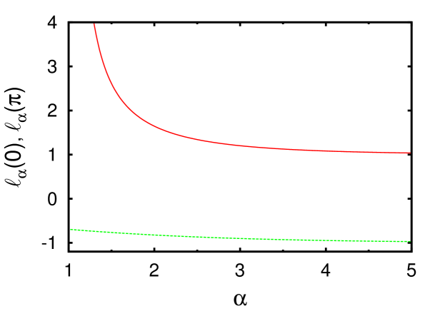
Figure 12: (Color online) Plot of $\ell_{\alpha}(0)$ [solid (red) line] and $\ell_{\alpha}(\pi)$ [dashed (green) line] as a function of $\alpha$.

The derivative of $\ell_{\alpha}$ has a different behavior for $1<\alpha<2$, $\alpha=2$ and $\alpha>2$. It is

$$\frac{\partial\ell_{\alpha}}{\partial q}\left(\pi\right)=0$$

for $\alpha>1$ and

$$\frac{\partial\ell_{\alpha}}{\partial q}\left(0\right)=\Bigg{\{}\begin{array}[]{cc}0&\alpha>2\\ -\frac{\pi}{2}&\alpha=2\\ -\infty&1<\alpha<2\end{array}$$ (43)

The second derivative of $\ell(\alpha)$ can be computed explicitly and it gives:

$$\frac{\partial^{2}\ell_{\alpha}}{\partial q^{2}}\left(q\right)=-\ell_{\alpha-2}(q).$$ (44)

For $1<\alpha\leq 2$ then $\frac{\partial^{2}\ell_{\alpha}}{\partial q^{2}}\left(q\right)$ is a positive function and we have $\frac{\partial^{2}\ell_{2}}{\partial q^{2}}\left(q\right)=\frac{1}{2}$, constant over $q\in[0,\pi]$. The second derivative takes the following values at the extrema of the interval $\left[0,\pi\right]$ for $\alpha>1$:

$$\frac{\partial^{2}\ell_{\alpha}}{\partial q^{2}}\left(0\right)=\left\{\begin{array}[]{cc}\infty&\alpha<2\\ 1/2&\alpha=2\\ -\infty&2<\alpha\leq 3\\ -\zeta(\alpha-2)&\alpha>3.\end{array}\right.$$ (45)

Finally at $q=\pi$ we have $\frac{\partial^{2}\ell_{\alpha}}{\partial q^{2}}\left(\pi\right)=(1-2^{3-\alpha})\zeta(\alpha)$ for every $\alpha>1$.

References

- (1) S. Flach and C. R. Willis, Phys. Rep. 295, 181 (1998).
- (2) O. Braun and Yu. S. Kivshar, Phys. Rep. 306, 1 (1998).
- (3) D. Hennig and G. P. Tsironis, Phys. Rep. 307, 333 (1999).
- (4) M. J. Ablowitz, B. Prinari, and A. D. Trubatch, Discrete and Continuous Nonlinear Schrödinger Systems (Cambridge University Press, Cambridge, England, 2004).
- (5) D. K. Campbell, S. Flach, and Y. S. Kivshar, Phys. Today 57, 43 (2004).
- (6) B. A. Malomed, Soliton Management in Periodic Systems (Springer, New York, 2006).
- (7) S. Flach and A. V. Gorbach, Phys. Rep. 467, 1 (2008).
- (8) T. B. Benjamin and J. E. Feir, J. Fluid. Mech. 27, 417 (1967).
- (9) G. P. Agrawal, Nonlinear Fiber Optics (Academic Press, Amsterdam, 2007).
- (10) Yu.S. Kivshar and M. Peyrard, Phys. Rev. A 46, 3198 (1992).
- (11) P. G. Kevrekidis, K. Ö Rasmussen, and A. R. Bishop, Int. J. Mod. Phys. B 15, 2833 (2001).
- (12) A. Trombettoni and A. Smerzi, Phys. Rev. Lett. 86, 2353 (2001).
- (13) H. S. Eisenberg, Y. Silberberg, R. Morandotti, A. R. Boyd, and J. S. Aitchison, Phys. Rev. Lett. 81, 3383 (1998).
- (14) A. Smerzi, A. Trombettoni, P. G. Kevrekidis, and A. R. Bishop, Phys. Rev. Lett. 89, 170402 (2002).
- (15) F. S. Cataliotti, L. Fallani, F. Ferlaino, C. Fort, P. Maddaloni, and M. Inguscio, New J. Phys. 5, 71 (2003).
- (16) J. Meier, G. I. Stegeman, D. N. Christodoulides, Y. Silberberg, R. Morandotti, H. Yang, G. Salamo, M. Sorel, and J. S. Aitchison, Phys. Rev. Lett. 92, 163902 (2004).
- (17) T. Lahaye, C. Menotti, L. Santos, M. Lewenstein, and T. Pfau, Rep. Prog. Phys. 72, 126401 (2009).
- (18) C. Trefzger, Menotti, B. Capogrosso-Sansone, and M. Lewenstein, J. Phys. B 44, 193001 (2011).
- (19) A. Griesmaier, J. Werner, S. Hensler, J. Stuhler, and T. Pfau, Phys. Rev. Lett. 94, 160401 (2005).
- (20) G. Bismut, B. Pasquiou, E. Marechal, P. Pedri, L. Vernac, O. Gorceix, and B. Laburthe-Tolra, Phys. Rev. Lett. 105, 040404 (2010).
- (21) M. Lu, N. Q. Burdick, S. H. Youn and B. L. Lev, Phys. Rev. Lett. 107, 190401 (2011).
- (22) S. Ospelkaus, K.-K. Ni, D. Wang, M. H. G. de Miranda, B. Neyenhuis, G. Quemener, P. S. Julienne, J. L. Bohn, D. S. Jin, and J. Ye, Science 327, 853 (2010).
- (23) R. Heidemann, U. Raitzsch, V. Bendkowsky, B. Butscher, R. Löw, and T. Pfau Phys. Rev. Lett. 100, 033601 (2008).
- (24) P. Schauß, M. Cheneau, M. Endres, T. Fukuhara, S. Hild, A. Omran, T. Pohl, C. Gross, S. Kuhr, and I. Bloch, Nature (London) 491, 87 (2012).
- (25) M. Saffman, T. G. Walker and K. Mølmer Rev. Mod. Phys. 82, 2313 (2010).
- (26) S. Müller, J. Billy, E. A. L. Henn, H. Kadau, A. Griesmaier, M. Jona-Lasinio, L. Santos, and T. Pfau, Phys. Rev. A 84, 053601 (2011).
- (27) J. Billy, E. A. L. Henn, S. Müller, T. Maier, H. Kadau, A. Griesmaier, M. Jona-Lasinio, L. Santos, and T. Pfau, Phys. Rev. A 86, 051603(R) (2012).
-
(28)
A. de Paz, A. Chotia, E. Marechal, P. Pedri, L. Vernac,
O. Gorceix, and B. Laburthe-Tolra,
arXiv:1212.5469 - (29) A. Chotia, B. Neyenhuis, S. A. Moses, B. Yan, J. P. Covey, M. Foss-Feig, A. M. Rey, D. S. Jin, and J. Ye, Phys. Rev. Lett. 108, 080405 (2012).
- (30) N. Henkel, R. Nath, and T. Pohl, Phys. Rev. Lett. 104, 195302 (2010).
- (31) M. Viteau, M. G. Bason, J. Radogostowicz, N. Malossi, D. Ciampini, O. Morsch, and E. Arimondo, Phys. Rev. Lett. 107, 060402 (2011).
- (32) Long-Range Interacting Systems: École d’Été de Physique des Houches, Session XC, edited by T. Dauxois, S. Ruffo, and L. F. Cugliandolo, (Oxford University Press, Oxford, 2010).
- (33) M. E. Fisher, S.-K. Ma, and B. G. Nickel, Phys. Rev. Lett. 29, 917 (1972).
- (34) J. Sak, Phys. Rev. B 8, 281 (1973).
- (35) E. Luijten and H. W. J. Blöte, Phys. Rev. Lett. 89, 025703 (2002).
- (36) A. Campa, T. Dauxois, and S. Ruffo, Phys. Rep. 480, 57 (2009).
- (37) J. M. Kosterlitz, Phys. Rev. Lett. 37, 1577 (1976).
- (38) H. Spohn and W. Zwerger, J. Stat. Phys. 94, 1037 (1996).
- (39) Y. B. Gaididei, S. F. Mingaleev, P. L. Christiansen, and K. Ø. Rasmussen, Phys. Rev. E 55, 6141 (1997).
- (40) S. Flach, Phys. Rev. E 58, R4116 (1998).
- (41) P. L. Christiansen, Y. B. Gaididei, M. Johansson, K. Ø. Rasmussen, V. K. Mezentsev, and J. J. Rasmussen, Phys. Rev. B 57, 11303 (1998).
- (42) S. F. Mingaleev, Y. S. Kivshar, and R. A. Sammut, Phys. Rev. E 62, 5777 (2000).
- (43) A. Fratalocchi and G. Assanto, Phys. Rev. E 72, 066608 (2005).
- (44) P. G. Kevrekidis, IMA J. Appl. Math. 76, 389 (2011).
- (45) J. M. Yeomans, Statistical Mechanics of Phase Transitions (Clarendon Press, Oxford, 1992).
- (46) F. J. Dyson, Comm. Math. Phys. 12, 91 (1969).
- (47) D. J. Thouless, Phys. Rev. 187, 732 (1969).
- (48) M. Le Bellac, Quantum and Statistical Field Theory (Clarendon Press, Oxford, 1991).
- (49) P. W. Anderson and G. Yuval, J. Phys. C: Solid State Phys. 4, 607 (1971).
- (50) E. Luijten and H. Meßingfeld: Phys. Rev. Lett. 86, 5305 (2001).
- (51) M. Seul and D. Andelman, Science 267, 476 (1995).
- (52) S. Chakrabarty and Z. Nussinov, Phys. Rev. B 84, 144402 (2011).
- (53) A. S. Davydov, Theory of Molecular Excitatons (Plenum, New York, 1971).
- (54) A. C. Scott, Phys. Rep. 217, 1 (1992).
- (55) M. Peyrard and A. R. Bishop, Phys. Rev. Lett. 62, 2755 (1989).
- (56) J. Cuevas, F. Palmero, J. F. R. Archilla, and F. R. Romero, Phys. Lett. A 299, 221 (2002).
-
(57)
S. Greschner, L. Santos, and T. Veuka,
arXiv:1202.5386 - (58) M. Olshanii, Phys. Rev. Lett. 81, 938 (1998).
- (59) S. Sinha and L. Santos, Phys. Rev. Lett. 99, 140406 (2007).
- (60) O. Morsch and M. Oberthaler, Rev. Mod. Phys. 78, 179 (2006).
- (61) D. van Oosten, P. van der Straten, and H. T. C. Stoof, Phys. Rev. A 63, 053601 (2001).
- (62) A. Trombettoni, A. Smerzi, and P. Sodano, New J. Phys. 7, 57 (2005).
- (63) E. G. Dalla Torre, E. Berg, and E. Altman, Phys. Rev. Lett. 97, 260401 (2006)
- (64) E. Berg, E. G. Dalla Torre, T. Giamarchi, and E. Altman, Phys. Rev. B 77, 245119 (2008).
- (65) L. Amico, G. Mazzarella, S. Pasini, and F.S. Cataliotti, New J. Phys. 12, 013002 (2010).
- (66) M. Dalmonte, M. Di Dio, L. Barbiero, and F. Ortolani, Phys. Rev. B 83, 155110 (2011).
- (67) D. Rossini and R. Fazio, New J. Phys. 14, 065012 (2012).
- (68) D. Giuliano, D. Rossini, P. Sodano, and A. Trombettoni, Phys. Rev. B 87, 035104 (2013).