Magnetic resonance spectroscopy and characterization of magnetic phases for spinor Bose-Einstein condensates

Abstract

The response of spinor Bose-Einstein condensates to dynamical modulation of magnetic fields is discussed with linear response theory. As an experimentally measurable quantity, the energy absorption rate (EAR) is considered, and the response function is found to access quadratic spin correlations which come from the perturbation of the quadratic Zeeman term. By applying our formalism to spin-$1$ condensates, we demonstrate that the EAR spectrum as a function of the modulation frequency is able to characterize the different magnetically ordered phases.

Introduction.— Ultracold Bose atoms with spin degrees of freedom Ho (1998); Ohmi and Machida (1998); Stamper-Kurn et al. (1998); Barrett et al. (2001); Ueda (2012); Kawaguchi and Ueda (2012); Stamper-Kurn and Ueda have been attracting interest as a class of quantum fluids accompanying nontrivial spin orders and topological spin textures, in contrast with spinless Bose-Einstein condensates (BECs). In BECs with spins, so-called spinor BECs, spin rotational symmetry allows spin-dependent interactions, and the number of the independent interactions increases with spin degrees of freedom of atoms, which causes various ground states. However, in addition to exploring the properties of those nontrivial spin orders, it is also important to specify their equilibrium properties experimentally. Thus, the development of measurement techniques to capture the physical properties of complicated ordered states is a challenge for the study of spinor BECs.

The powerful way to identify the mean-field ground state and the phase diagrams is the measurement of population of the spin components by the combination of the Stern-Gerlach experiment and time-of-flight (TOF) analysis. Stenger et al. (1998); Black et al. (2007); Kuwamoto et al. (2004); Chang et al. (2004); Schmaljohann et al. (2004); Pasquiou et al. (2011) In addition, the dispersive imaging method with off-resonant light allows for displaying spatially resolved spin profiles Carusotto and Mueller (2004); Higbie et al. (2005); Liu et al. (2009); Kuzmich et al. (1999). At the same time, while the current techniques probe equilibrium properties, it is also challenging to provide more direct and systematic probes to visualize the excitation energy structure coming from spin fluctuations.

For spinor BECs in the presence of uniform magnetic fields, the quadratic Zeeman (QZ) shift, in addition to the linear Zeeman (LZ) shift, emerges due to hyperfine couplings between a nuclear and an electron spin Stenger et al. (1998). Because the magnetization of spinor BECs is known to be preserved at least within the limit of accuracy of experimental errors Chang et al. (2004), the QZ shift is the most relevant effect induced by the magnetic field. In addition and importantly, the QZ coupling is experimentally controllable Gerbier et al. (2006); Leslie et al. (2009); Bookjans et al. (2011); Jacob et al. (2012); Sadler et al. (2006); Guzman et al. (2011).

In this Rapid Communication, motivated by such a possible control of the QZ coupling, we consider magnetic resonant spectra as a response to dynamically modulated magnetic fields, which possesses the potential to probe microscopic spin-excitation energy structures. As a measurable quantity, we focus on the energy absorption rate (EAR), and formulate it with linear response theory. The consequent formula is applicable to general systems with any spin degree of freedom. This type of resonance spectra has not been considered, and thus it is important to clarify the spectral features for various states. As a simple case, we take spin-$1$ BECs in this Rapid Communication and calculate the spectrum with Bogoliubov theory Murata et al. (2007); Uchino et al. (2010). As a result, they are found to exhibit different behaviors in each phase. Furthermore, we also consider the cases in the presence of trap potentials and a noncondensed fraction, and the ordered states are concluded to remain distinguishable from the low-frequency behaviors of the EAR spectra.

Formalism.— We start with general spin-$F$ Bose atom systems under a uniform magnetic field. Let us suppose the many-body static Hamiltonian including Zeeman couplings to be $H_{0}$. In this Rapid Communication, we restrict ourselves to the cases for which the magnetic field is applied along the $z$ axis, and $H_{0}$ is invariant under spin rotation around the $z$ axis, which is a general setup in experiments.

In the presence of a dynamically modulated magnetic field such as $h+\delta{h}\cos(\omega t/2)$, the system should be described by the time-dependent Hamiltonian $H(t)=H_{0}+V(t)$, and the perturbation is represented as

$$V(t)=(\delta{p})\cos(\omega t/2)\mathcal{F}_{\mathrm{L}}+(\delta{q})\cos^{2}(\omega t/2)\mathcal{F}_{\mathrm{Q}},$$ (1)

where the first and second terms mean modulation of the LZ and QZ couplings, respectively. The coupling constants, $\delta{p}$ and $\delta{q}$, are proportional to $\delta{h}$ and $(\delta{h})^{2}$, respectively. The LZ and QZ operators are represented as

$$\mathcal{F}_{\mathrm{L}}=\int\!\!d\bm{r}\,\hat{\Psi}^{\dagger}(\bm{r})F^{z}\hat{\Psi}(\bm{r}),$$ (2)

$$\mathcal{F}_{\mathrm{Q}}=\int\!\!d\bm{r}\,\hat{\Psi}^{\dagger}(\bm{r})(F^{z})^{2}\hat{\Psi}(\bm{r}),$$ (3)

where $\hat{\Psi}=(\psi_{F},\psi_{F-1},\cdots,\psi_{-F})^{T}$ denotes a spinor boson field, and $\bm{F}=(F^{x},F^{y},F^{z})$ is a spin-$F$ matrix.

In experiments, the EAR can be measured through the TOF image. Assuming the energy scale of the periodically modulated perturbation is small enough , the dynamics is well described with linear response theory. Then, the EAR is defined as $R(\omega)=\frac{1}{2\pi/\omega}\int_{T}^{T+2\pi/\omega}\!\!d{t}\frac{d\braket{H(t)}}{dt}$, where $\braket{\cdots}$ denotes the statistical average over $H(t)$. Thus, the EAR is derived as

$$R(\omega)=-\frac{1}{2\hbar}\omega\mathrm{Im}[\chi^{\mathrm{R}}(\omega)],$$ (4)

where $\chi^{\mathrm{R}}(\omega)=-i\int_{0}^{\infty}dt\,e^{i\omega t}\braket{[V(t),V(0)]}_{0}$ is the retarded correlation function of the perturbation (1) averaged over $H_{0}$. Since $H_{0}$ is assumed to possess the spin rotational symmetry around the $z$ axis, $[\mathcal{F}_{\mathrm{L}},H_{0}]=[\mathcal{F}_{\mathrm{L}},\mathcal{F}_{\mathrm{Q}}]=0$, and thus the retarded correlation function is reduced to

$$\chi^{\mathrm{R}}(\omega)=-i(\delta{q})^{2}\int_{0}^{\infty}\!\!d{t}\,e^{i\omega t}\braket{[\mathcal{F}_{\mathrm{Q}}(t),\mathcal{F}_{\mathrm{Q}}(0)]}_{0}.$$ (5)

Namely, the system is insensitive to the dynamic modulation of the LZ coupling. The remarkable point here is that the obtained formula is generic, and applicable for any spin degrees of freedom and form of interactions, as long as the uniaxial spin rotational symmetry exists at least.

EAR for spin-$1$ BECs.— Let us demonstrate the EAR spectrum (4) to allow for characterizing spin-ordered phases. We consider spin-$1$ interacting bosons Ho (1998); Ohmi and Machida (1998); Stenger et al. (1998) without a trap, which undergo a BEC in the low-temperature regime . Hereafter, we fix total spin to be zero.  Then, since the LZ term is effectively vanished Stenger et al. (1998), the Hamiltonian to be considered is given by

$$H_{0} =\int\!\!d\bm{r}\,\biggl{[}-\frac{\hbar^{2}}{2M}\hat{\Psi}^{\dagger}(\bm{r})\nabla^{2}\hat{\Psi}(\bm{r})+q\hat{\Psi}^{\dagger}(\bm{r})(F^{z})^{2}\hat{\Psi}(\bm{r})$$

$$\quad+\frac{c_{0}}{2}\Bigl{(}\hat{\Psi}^{\dagger}(\bm{r})\hat{\Psi}(\bm{r})\Bigr{)}^{2}+\frac{c_{1}}{2}\Bigl{(}\hat{\Psi}^{\dagger}(\bm{r})\bm{F}\hat{\Psi}(\bm{r})\Bigr{)}^{2}\biggr{]},$$ (6)

where $\hat{\Psi}=(\psi_{1},\psi_{0},\psi_{-1})^{T}$, $M$ denotes the mass of the atoms, and $c_{0}$ and $c_{1}$ mean the density and spin exchange interactions, respectively. For ²³Na and ⁸⁷Rb atoms, the coupling $c_{1}$ is taken to be a positive and negative value, respectively. Let us impose $nc_{0}\gg n|c_{1}|,|q|$, where $n$ is the atom density corresponding to the experimental conditions. Since the EAR is independent of the LZ coupling modulation, as discussed above, instead of (1) we here suppose the modulation perturbation of the magnetic field to be

$$V(t)=(\delta{q})\cos(\omega t)\mathcal{F}_{\mathrm{Q}}.$$ (7)

The mean-field (MF) analysis, in which the field $\hat{\Psi}$ is replaced by a MF spinor order parameter $\hat{\xi}$ optimizing the Hamiltonian (6), leads to the following ground states Uchino et al. (2010)  as shown in Fig. 1: (i) the ferromagnetic (FM) phase $\hat{\xi}_{\mathrm{FM}}=(1,0,0)^{T}$ for $c_{1},q<0$, (ii) the longitudinal polar (LP) phase $\hat{\xi}_{\mathrm{LP}}=(0,1,0)^{T}$ for $q>0$ and $q+2nc_{1}>0$, (iii) the transverse polar (TP) phase $\hat{\xi}_{\mathrm{TP}}=(1/\sqrt{2},0,1/\sqrt{2})^{T}$ for $c_{1}>0$ and $q<0$, and (iv) the broken-axisymmetry (BA) phase $\hat{\xi}_{\mathrm{BA}}=(\sin{\theta}/\sqrt{2},\cos{\theta},\sin{\theta}/\sqrt{2})^{T}$, where $\sin{\theta}=\sqrt{(1-\tilde{q})/2}$ with $\tilde{q}=q/(2n|c_{1}|)$, for $c_{1}<0$ and $0<q<2n|c_{1}|$.

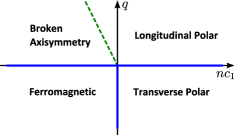
Figure 1: (Color online) The MF phase diagram of spin-$1$ BECs with respect to the effective spin-exchange interaction $nc_{1}$ and QZ coupling $q$, which are here restricted to being weak compared with the density interaction, i.e., $|q|,\,n|c_{1}|\ll nc_{0}$. The thick-solid and dashed boundary lines denote first- and second-order phase transitions, respectively. We note that the phase diagram was first given in Stenger et al. (1998), which covers a wider parameter regime than shown here. The phase boundary between the BA and LP phase is given by $q=2n|c_{1}|$.

The correlation function $\chi^{\mathrm{R}}(\omega)$ is calculated with the Bogoliubov theory by the replacement $\hat{\Psi}=\sqrt{N_{0}}\hat{\bm{\xi}}_{\alpha}+\delta{\hat{\Psi}}$ ($\alpha=\mathrm{FM},\mathrm{LP},\mathrm{TP},\mathrm{BA}$), where $N_{0}$ is the condensate atom number. Then the Bogoliubov Hamiltonian is represented as $H_{0}\approx E_{\mathrm{MF}}+H_{\mathrm{eff}}$, with the MF energy $E_{\mathrm{MF}}$ and

$$H_{\mathrm{eff}} =\sum_{\bm{k}\neq\bm{0}}\biggl{[}\hat{a}^{\dagger}_{\bm{k}}\Bigl{(}\epsilon_{\bm{k}}+nc_{1}\overline{\bm{F}}\cdot(\bm{F}-\overline{\bm{F}})+q((F^{z})^{2}-\overline{(F^{z})^{2}})\Bigr{)}\hat{a}_{\bm{k}}$$

$$\quad+\frac{nc_{0}}{2}\Bigl{(}D^{\dagger}_{\bm{k}}D_{\bm{k}}+D_{\bm{k}}D_{-\bm{k}}+\mathrm{H.c}\Bigr{)}$$

$$\quad+\frac{nc_{1}}{2}\Bigl{(}\bm{S}^{\dagger}_{\bm{k}}\cdot\bm{S}_{\bm{k}}+\bm{S}_{\bm{k}}\cdot\bm{S}_{-\bm{k}}+\mathrm{H.c}\Bigr{)}\biggr{]},$$ (8)

where $\epsilon_{\bm{k}}=\frac{\hbar^{2}\bm{k}^{2}}{2M}$, and $\hat{a}_{\bm{k}}=\int\!\!d\bm{r}e^{i\bm{k}\cdot\bm{r}}\delta{\hat{\Psi}}=(a_{1\bm{k}},a_{0\bm{k}},a_{-1\bm{k}})^{T}$ is a Fourier transform of the spinor fluctuation. $D_{\bm{k}}=\hat{\xi}^{\dagger}\hat{a}_{\bm{k}}$ and $\bm{S}_{\bm{k}}=\hat{\xi}^{\dagger}\bm{F}\hat{a}_{\bm{k}}$ mean density and spin fluctuations, respectively, and $\overline{X}=\hat{\xi}^{\dagger}X\hat{\xi}$, for a spin operator $X$, denotes the MF average of spin matrices. In this representation, the QZ operator is expressed as

$$\mathcal{F}_{\mathrm{Q}}=N\overline{(F^{z})^{2}}+\sum_{\bm{k}\neq\bm{0}}\hat{a}^{\dagger}_{\bm{k}}\left[(F^{z})^{2}-\overline{(F^{z})^{2}}\right]\hat{a}_{\bm{k}},$$ (9)

where $N$ denotes the atom number.

FM phase.— The MF spinor leads to the density and spin fluctuation as $D_{\bm{k}}=S^{z}_{\bm{k}}=a_{1\bm{k}}$, $S^{x}_{\bm{k}}=a_{0\bm{k}}/\sqrt{2}$, and $S^{y}_{\bm{k}}=ia_{0\bm{k}}/\sqrt{2}$. The effective Hamiltonian diagonalized by the Bogoliubov transformation is given Uchino et al. (2010) as

$$H^{\mathrm{FM}}_{\mathrm{eff}} =\sum_{\bm{k}\neq\bm{0}}\biggl{[}E^{\mathrm{FM}}_{\mathrm{d}}(\bm{k})d^{\dagger}(\bm{k})d(\bm{k})+E^{\mathrm{FM}}_{z}(\bm{k})f^{\dagger}_{z}(\bm{k})f_{z}(\bm{k})$$

$$\quad+E^{\mathrm{FM}}_{xy}(\bm{k})f^{\dagger}_{xy}(\bm{k})f_{xy}(\bm{k})\biggr{]},$$ (10)

where $E^{\mathrm{FM}}_{\mathrm{d}}(\bm{k})=\sqrt{\epsilon_{\bm{k}}[\epsilon_{\bm{k}}+2n(c_{0}-|c_{1}|)]}$, $E^{\mathrm{FM}}_{z}(\bm{k})=\epsilon_{\bm{k}}+2n|c_{1}|$, and $E^{\mathrm{FM}}_{xy}(\bm{k})=\epsilon_{\bm{k}}+|q|$. The QZ operator in the FM phase is written as

$$\mathcal{F}^{\mathrm{FM}}_{\mathrm{Q}}=\mathrm{Const.}+\sum_{\bm{k}\neq\bm{0}}f^{\dagger}_{xy}(\bm{k})f_{xy}(\bm{k}).$$ (11)

Since the perturbation $\mathcal{F}^{\mathrm{FM}}_{\mathrm{Q}}$ commutes with the Hamiltonian (10), $\chi^{\mathrm{R}}(\omega)$ is immediately found to be zero. Thus, the EAR spectrum shows no signal in the entire $\omega$ regime.

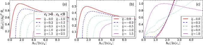
Figure 2: (Color online) The EAR spectra as a function of modulation frequency for the different $\tilde{q}=q/2n|c_{1}|$: (a) the LP phase for $c_{1},q>0$ or for $q>0$ and $q+2nc_{1}>0$, (b) the TP phase for $c_{1}>0$ and $q<0$, and (c) the BA phase for $c_{1}<0$ and $0<q<2n|c_{1}|$. Spectra (a) and (b) are qualitatively the same, but the intensity differs due to the different number of accessible gapful-spin modes. Spectra (c) apart from $\tilde{q}=1$ show an abrupt enhancement of the EAR around $\hbar\omega\approx 2n|c_{1}|$, which indicates the appearance of the contribution from $r_{\mathrm{BA}_{\mathrm{d}}}(\omega)$.

LP phase.— The diagonalized Bogoliubov Hamiltonian is given (see Uchino et al. (2010) and Supplemental Material sm ) as

$$H^{\mathrm{LP}}_{\mathrm{eff}}=\sum_{\bm{k}\neq\bm{0}}\left[E_{\bm{k}}d^{\dagger}(\bm{k})d(\bm{k})+\sum_{\nu=x,y}E^{f}_{\bm{k}}f^{\dagger}_{\nu}(\bm{k})f_{\nu}(\bm{k})\right],$$ (12)

where $E_{\bm{k}}=\sqrt{\epsilon_{\bm{k}}(\epsilon_{\bm{k}}+2nc_{0})}$ and $E^{f}_{\bm{k}}=\sqrt{(\epsilon_{\bm{k}}+|q|)(\epsilon_{\bm{k}}+|q|+2nc_{1})}$ are, respectively, a gapless-phonon and doubly degenerate gapful-spin mode. The Bogoliubov transformation gives the form of the QZ perturbation (see Supplemental Material sm ) as

$$\mathcal{F}^{\mathrm{LP}}_{\mathrm{Q}} =\bar{\mathcal{F}}^{\mathrm{LP}}_{\mathrm{Q}}-\sum_{\bm{k}\neq\bm{0}}\sum_{\nu=x,y}\mathcal{A}^{\mathrm{LP}}_{\bm{k}}\biggl{[}f^{\dagger}_{\nu}(\bm{k})f^{\dagger}_{\nu}(-\bm{k})+\mathrm{H.c.}\biggr{]},$$ (13)

where $\bar{\mathcal{F}}^{\mathrm{LP}}_{\mathrm{Q}}$ contains terms which commute with the Hamiltonian (12), and $\mathcal{A}^{\mathrm{LP}}_{\bm{k}}=n|c_{1}|/2E^{f}_{\bm{k}}$. The QZ perturbation accesses the two spin modes. From Eq. (13), the retarded correlation function is straightforwardly calculated, and consequently the EAR spectrum is analytically obtained (see Supplemental Material sm ) as $R_{\mathrm{LP}}(\omega)=(\delta{q})^{2}\mathcal{R}_{\mathrm{c}}\theta_{\mathrm{H}}(|\tilde{\omega}|-2\tilde{\Delta}_{q})r_{\mathrm{LP}}(\omega)$ with

$$r_{\mathrm{LP}}(\omega)=2\sqrt{\frac{\sqrt{1+\tilde{\omega}^{2}}-2\tilde{q}-\mathrm{sgn}(c_{1})}{1+\tilde{\omega}^{2}}},$$ (14)

where $\theta_{\mathrm{H}}(x)$ is a Heaviside step function, and $\mathcal{R}_{\mathrm{c}}=\Omega(2Mn|c_{1}|)^{3/2}/64\pi\hbar^{4}$ with the system volume $\Omega$ is a constant. We have taken $\tilde{\omega}=\hbar\omega/2n|c_{1}|$, $\tilde{q}=q/2n|c_{1}|$, and $\tilde{\Delta}_{q}=\sqrt{|\tilde{q}|(|\tilde{q}|+\mathrm{sgn}(c_{1}))}$. The spin gap in the polar phase has been denoted by $2n|c_{1}|\tilde{\Delta}_{q}$. Equation (14) for various values of $q$ is plotted in Fig. 2(a). Note that the gap of the EAR spectrum closes on the phase boundaries, $q=0$ with $c_{1}>0$ and $q=2n|c_{1}|$ with $c_{1}<0$.

TP phase.— The Bogoliubov transformation diagonalizes the Hamiltonian (see Uchino et al. (2010) and Supplemental Material sm as

$$H^{\mathrm{TP}}_{\mathrm{eff}}=\sum_{\bm{k}\neq\bm{0}}\left[E_{\bm{k}}d^{\dagger}(\bm{k})d(\bm{k})+E^{z}_{\bm{k}}f_{z}^{\dagger}(\bm{k})f_{z}(\bm{k})+E^{f}_{\bm{k}}f^{\dagger}(\bm{k})f(\bm{k})\right],$$ (15)

where $E_{\bm{k}}$ and $E^{z}_{\bm{k}}=\sqrt{\epsilon_{\bm{k}}(\epsilon_{\bm{k}}+2nc_{1})}$ are gapless modes of phonon and spin, respectively, and $E^{f}_{\bm{k}}$ is another spin mode with the gap $\tilde{\Delta}_{q}$. The QZ operator is written (see Supplemental Material sm ) as

$$\mathcal{F}^{\mathrm{TP}}_{\mathrm{Q}} =\bar{\mathcal{F}}^{\mathrm{TP}}_{\mathrm{Q}}-\sum_{\bm{k}\neq\bm{0}}\mathcal{A}^{\mathrm{TP}}_{\bm{k}}\biggl{[}f^{\dagger}(\bm{k})f^{\dagger}(-\bm{k})+\mathrm{H.c.}\biggr{]},$$ (16)

where $\bar{\mathcal{F}}^{\mathrm{TP}}_{\mathrm{Q}}$ denotes terms which commute with the Hamiltonian (15), and $\mathcal{A}^{\mathrm{TP}}_{\bm{k}}=nc_{1}/2E^{f}_{\bm{k}}$. From Eq. (16), the QZ modulation is found to access only one gapful-spin mode. Straightforwardly, the retarded correlation function of Eq. (16) is calculated and the EAR is analytically obtained (see Supplemental Material sm ) as $R_{\mathrm{TP}}(\omega)=(\delta{q})^{2}\mathcal{R}_{\mathrm{c}}\theta_{\mathrm{H}}(|\tilde{\omega}|-2\tilde{\Delta}_{q})r_{\mathrm{TP}}(\omega)$ with

$$r_{\mathrm{TP}}(\omega) =\sqrt{\frac{\sqrt{1+\tilde{\omega}^{2}}-2|\tilde{q}|-1}{1+\tilde{\omega}^{2}}},$$ (17)

which is illustrated in Fig. 2.

It is remarkable that for positive $c_{1}$, we have $R_{\mathrm{LP}}(\omega)/R_{\mathrm{TP}}(\omega)=2$ for the fixed $|q|$, and the factor $2$ is a robust number because it comes from the accessible number of the spin modes by the QZ perturbation; namely, the perturbation (13) for the LP phase involves the two gapful-spin modes, while only one gapful-spin mode is accessed for the TP phase. Although the two polar phases just have a quantitative difference and other calibration may be needed to explicitly differentiate them through a single measurement under a certain $|q|$, the different spectral intensity still has an interesting aspect: If we continuously change $q$ across $q=0$, a discontinuous spectrum change is observed, and it would be interpreted to be a signal of the first-order phase transition associated with the spontaneous symmetry breaking between the two different polar directions.

In summary, the EAR in the polar phases has two important features: The first is that we can measure the spin gap $\tilde{\Delta}_{q}$ which dominates the low-energy spin excitation. The second is that the discontinuous difference of the spectral intensity allows for observing the first order phase transition from the dynamical viewpoint. As we will discuss later, these conclusions do not change even if we have trap potentials.

BA phase.— For $c_{0}\gg|c_{1}|$, the Bogoliubov Hamiltonian is diagonalized (see Uchino et al. (2010); Murata et al. (2007); Barnett et al. (2011) and Supplemental Material sm as

$$H^{\mathrm{BA}}_{\mathrm{eff}} =\sum_{\bm{k}\neq\bm{0}}\biggl{[}E^{\mathrm{BA}_{\mathrm{d}}}_{\bm{k}}d^{\dagger}(\bm{k})d(\bm{k})+E^{\mathrm{BA}_{z}}_{\bm{k}}f^{\dagger}_{z}(\bm{k})f_{z}(\bm{k})$$

$$\quad+E^{\mathrm{BA}_{xy}}_{\bm{k}}f^{\dagger}_{xy}(\bm{k})f_{xy}(\bm{k})\biggr{]},$$ (18)

where $E^{\mathrm{BA}_{\mathrm{d}}}_{\bm{k}}=\sqrt{\epsilon_{\bm{k}}[\epsilon_{\bm{k}}+2nc_{0}-2n|c_{1}|(1-\tilde{q}^{2})]}$, $E^{\mathrm{BA}_{z}}_{\bm{k}}=\sqrt{\epsilon_{\bm{k}}(\epsilon_{\bm{k}}+q)}$, and $E^{\mathrm{BA}_{xy}}_{\bm{k}}=\sqrt{(\epsilon_{\bm{k}}+2n|c_{1}|)[\epsilon_{\bm{k}}+2(1-\tilde{q}^{2})n|c_{1}|]}$ are interpreted to be the density mode, the gapless-spin mode and the gapful-spin mode, respectively. The QZ perturbation is represented (see Supplemental Material sm ) as

$$\mathcal{F}_{\mathrm{Q}}^{\mathrm{BA}} =\bar{\mathcal{F}}^{\mathrm{BA}}_{\mathrm{Q}}+\sum_{\bm{k}\neq\bm{0}}\biggl{[}-\mathcal{A}^{\mathrm{BA}}_{\bm{k}}f_{z}(\bm{k})f_{z}(-\bm{k})+\mathcal{B}^{\mathrm{BA}}_{\bm{k}}f^{\dagger}_{xy}(\bm{k})d(\bm{k})$$

$$\quad+\mathcal{C}^{\mathrm{BA}}_{\bm{k}}f_{xy}(\bm{k})f_{xy}(-\bm{k})+\mathcal{D}^{\mathrm{BA}}_{\bm{k}}f_{xy}(\bm{k})d(-\bm{k})+\mathrm{H.c.}\biggr{]},$$ (19)

where $\bar{\mathcal{F}}^{\mathrm{BA}}_{\mathrm{Q}}$ commutes with the Hamiltonian (18), and the factors are $\mathcal{A}^{\mathrm{BA}}_{\bm{k}}=q/4E^{\mathrm{BA}_{z}}_{\bm{k}}$, $\mathcal{B}^{\mathrm{BA}}_{\bm{k}}=-\frac{\sin{2\theta}}{4}[\sqrt{\alpha_{\bm{k}}\beta_{\bm{k}}}+\frac{1}{\sqrt{\alpha_{\bm{k}}\beta_{\bm{k}}}}]$, $\mathcal{C}^{\mathrm{BA}}_{\bm{k}}=-\frac{\tilde{q}}{4}[\alpha_{\bm{k}}-\frac{1}{\alpha_{\bm{k}}}]$, $\mathcal{D}^{\mathrm{BA}}_{\bm{k}}=\frac{\sin{2\theta}}{4}[\sqrt{\alpha_{\bm{k}}\beta_{\bm{k}}}-\frac{1}{\sqrt{\alpha_{\bm{k}}\beta_{\bm{k}}}}]$, $\alpha_{\bm{k}}=E^{\mathrm{BA}_{xy}}_{\bm{k}}/(\epsilon_{\bm{k}}+2n|c_{1}|)$, and $\beta_{\bm{k}}=E^{\mathrm{BA_{d}}}_{\bm{k}}/\epsilon_{\bm{k}}$. Equation (19) leads to the EAR $R^{\mathrm{BA}}(\omega)=(\delta{q})^{2}\mathcal{R}_{\mathrm{c}}[r_{\mathrm{BA}_{z}}(\omega)+\theta_{\mathrm{H}}(|\tilde{\omega}|-2\tilde{\Delta}_{q}^{\mathrm{BA}})r_{\mathrm{BA}}(\omega)+\theta_{\mathrm{H}}(|\tilde{\omega}|-\tilde{\Delta}_{q}^{\mathrm{BA}})r_{\mathrm{BA}_{\mathrm{d}}}(\omega)]$ with

$$r_{\mathrm{BA}_{z}}(\omega) =\tilde{q}^{2}\sqrt{\frac{\sqrt{\tilde{q}^{2}+\tilde{\omega}^{2}}-\tilde{q}}{\tilde{q}^{2}+\tilde{\omega}^{2}}},$$ (20)

$$r_{\mathrm{BA}_{xy}}(\omega) =\tilde{q}^{6}\sqrt{\frac{\sqrt{\tilde{q}^{4}+\tilde{\omega}^{2}}+\tilde{q}^{2}-2}{\tilde{q}^{4}+\tilde{\omega}^{2}}},$$ (21)

$$r_{\mathrm{BA}_{\mathrm{d}}}(\omega) =\left(\frac{2|c_{1}|}{c_{0}}\right)^{3/2}\left(\tilde{\Delta}_{q}^{\mathrm{BA}}\right)^{2}|\tilde{\omega}|$$

$$\quad\times\left(|\tilde{\omega}|-\tilde{\Delta}_{q}^{\mathrm{BA}}\right)^{2}\left[\gamma(\omega)-\frac{1}{\gamma(\omega)}\right]^{2},$$ (22)

where $\gamma(\omega)=\sqrt{\frac{(c_{0}/|c_{1}|)^{2}\tilde{\Delta}_{q}^{\mathrm{BA}}}{(|\tilde{\omega}|-\tilde{\Delta}_{q}^{\mathrm{BA}})[(|\tilde{\omega}|-\tilde{\Delta}_{q}^{\mathrm{BA}})^{2}+c_{0}/|\tilde{c}_{1}|]}}$. $2n|c_{1}|\tilde{\Delta}_{q}^{\mathrm{BA}}=\sqrt{(2nc_{1})^{2}-q^{2}}$ denotes the energy gap of the spin mode, $E^{\mathrm{BA}_{xy}}_{\bm{k}}$ (see Supplemental Material sm ).

The EAR spectra for the various $\tilde{q}$’s in the BA phase are shown in Fig. 2(c). The gapless spectral weight $r_{\mathrm{BA}_{z}}(\omega)$ describes a two-particle excitation of the gapless-spin mode $E^{\mathrm{BA}_{z}}_{\bm{k}}$, and at the limit $\tilde{q}\rightarrow 1$, it is identical to $R_{\mathrm{TP}}(\omega)$ at $\tilde{q}\rightarrow 1$. The weight $r_{\mathrm{BA}_{xy}}(\omega)$, which is the two-particle excitation of the spin mode $E^{\mathrm{BA}_{xy}}_{\bm{k}}$, gives the gapful EAR spectrum with the gap, $2\tilde{\Delta}_{q}^{\mathrm{BA}}$, and vanishes at the limit $\tilde{q}\rightarrow 0$. The other spectrum weight $r_{\mathrm{BA}_{\mathrm{d}}}(\omega)$ from the pair excitation of the quasiparticles of the gapless-phonon mode $E^{\mathrm{BA}_{\mathrm{d}}}_{\bm{k}}$ and of the gapful-spin mode $E^{\mathrm{BA}_{z}}_{\bm{k}}$ provides a gapful spectrum with the gap $\tilde{\Delta}_{q}^{\mathrm{BA}}$. The two-particle excitation of the spin and density mode is peculiar to the BA phase, as seen in the form of the QZ perturbation (19). In addition, the spectrum weight $r_{\mathrm{BA}_{\mathrm{d}}}(\omega)$ is of the order of $\sqrt{c_{0}/|c_{1}|}$, while the others are independent of $c_{0}$. Thus, the EAR for $c_{0}\gg|c_{1}|$ is dominated by $r_{\mathrm{BA}_{\mathrm{d}}}(\omega)$ in the frequency regime where $r_{\mathrm{BA}_{\mathrm{d}}}(\omega)$ is finite.

Trap effect.— Based on the above results in the homogeneous case, we discuss the EAR spectrum for trapped systems by local density approximation. Then, the spectrum is calculated by taking the average of the local spectrum with the weight of the local density $n(\bm{r})$. The local EAR is obtained by replacing the mean density $n$ by the local one $n(\bm{r})$. Since the density $n$ accompanies the interaction constant $c_{0}$ and $c_{1}$ in all of the results, it turns out that the inhomogeneity modifies the strength of the interactions: The effective interaction around the trap center is stronger at the center, and gets weaker when going away from the center. Thus, if the trap center is in the polar phase and in the FM, the whole system exhibits a polar and FM state, respectively, as expected from Fig. 1. In addition, since the gap of the EAR spectrum is independent of the density and the interaction, the gapful feature of the EAR in the polar phases should remain even in the trapped case. On the other hand, when the trap center is in the BA phase, the outward regime would be a polar state. However, since the EAR in the BA phase is characterized by the gapless spectrum, the qualitative feature is expected to be protected. Therefore, the EAR spectrum is concluded to characterize the phases of spin-$1$ BECs regardless of the presence of trap potentials.

Effect of noncondensed fraction.— In spinor BECs, it may not be so trivial that the effect of noncondensed atoms is negligible. Phuc et al. (2011) Such a noncondensed fraction can be regarded as some kind of fluctuation, and the Bogoliubov spectra is thus expected to capture the physics. Since the main features of the obtained spectra come from the spectral character of the fluctuations, they should be visible even in the presence of the noncondensed fraction. Therefore, if the system is cooled down enough such that the temperature is less than the mean-field energy, the spectra demonstrated here would be measured due to the bosonic stimulation effect.

Conclusion.— We have formulated the response of the spinor BECs to modulation of the magnetic field by using linear response theory, which gives access to the correlation of the QZ term, and, by considering the spin-$1$ BECs, the spectrum has been demonstrated to have individual features in each magnetic phase. In addition, the results have been found robust against the trap effect.

Finally, we comment on potential applications of this spectroscopy. From the high versatility of the formula (4), it can be widely applied, for example, to BECs with any spin, high-spin Fermi atoms, and optical lattice systems. Furthermore, it would also be used for the following fundamental problems: an experimental test to verify Bogoliubov theory for spinor BECs, and dimensionality discussion on single- and multispatial spin modes for an anisotropic trap by using the fact that the different spectral shape strongly depends on the system dimensions.